Noise Source Identification For Ducted Fan Systems (AIAA 2007 3693)

Noise Source Identification for Ducted Fan Systems

Gareth J. Bennett

_{and John A. Fitzpatrick}

Trinity College Dublin, Dublin 2, Ireland.

Understanding combustion noise source mechanisms, designing efficient acoustic liners and optimising active control algorithms for noise reduction requires the identification of the frequency and modal content of the combustion noise contribution. Coherence-based noise source identification techniques have been developed which can be used to identify the contribution of combustion noise to near and far-field acoustic measurements of aero-engines. A number of existing identification techniques from the literature are implemented and evaluated under controlled experimental conditions. An experimental rig was designed and built to gain a fundamental physical understanding of the convection of noise through a rotor/stator set-up. The identification techniques were applied to this rig and the pressure field was separated into its constituent parts.

The underlying assumption with these identification techniques is that the propaga-tion/convection path, from combustion can to measurement point, is a linear one. It is shown with simulations that where the combustion noise propagates in a non-linear fashion the identified contribution will be inaccurate. The experimental rig, consisting of a vane-axial fan mounted in a duct, allows potential non-linear interaction mechanisms between a convected sound source and the fan to be investigated. Tests carried out on the experi-mental rig allowed a non-linear interaction tone, between the rotor BPF and a convected tone, to be generated.

An experimental technique was developed which enabled the non-linear interaction be-tween the convected sound source with the vane-axial fan to be detected and identified when present. The technique was extended to allow the linear and non-linear acoustic contributions to be separated. The capacity to decompose the coherent output power into linear and non-linear components is a useful tool for the correct design of acoustic treatment for core noise and for an accurate identification of noise source generating mechanisms.

The non-linear identification techniques, developed with the experimental rig, were ap-plied to data from full scale turbo-fan engine tests. A Rolls-Royce engine was instrumented with pressure transducers at the combustor can and in the hot-jet pipe, and microphones were placed in the near-field. For a particular power setting, frequency scattering was seen to occur between the combustion noise and the high pressure turbine which was measur-able in the hot jet pipe after convection through the many turbine stages. The techniques allowed the non-linear interaction to be successfully identified and linear and non-linear coherent output powers to be determined.

Nomenclature

γij2 Ordinary Coherence Function between signals i(t) and j(t)

Gij Averaged single-sided power cross-spectral density between signals i(t) and j(t)

x:i The part of x correlated with i

x·i Conditioned record or the residual. The part of x not correlated with i HPT High Pressure Turbine

LPT Low Pressure Turbine ∗_{Research Fellow.}

I.

Introduction

The two principal sources of aero-engine noise, the fan and the jet, have been significantly reduced over many years of research. With their reduction, a threshold which will form the new noise floor is being reached and this will limit the benefits to be gained by further reducing these dominant components, unless the noise sources which set this threshold are in turn reduced. Of these, combustion, or core noise, is an area of current research activity. At relatively low jet velocities, such as would occur at engine idle, during taxiing, and at approach and cruise conditions, core noise is considered a significant contributor to the overall sound level. It will continue to receive attention as the current trend towards high-bypass engines and low Nox combustors will result in the core noise becoming a more significant source.

Understanding combustion noise source mechanisms, designing efficient acoustic liners and optimising active control algorithms for noise reduction requires the identification of the frequency and modal content of the combustion noise contribution. An acoustic measurement of a system of interest will most often be the summation of a number of separate acoustic sources along with some extraneous noise. For the case where it is not possible to remove individual sources without affecting the behaviour of the others, the challenge is to decompose the measurement signal into its constituent parts. As the acoustic noise sources in an aero-engine overlap in the frequency domain, with varying amplitudes, it can be difficult to quantify the individual contributions.

Coherence-based noise source identification techniques can be used to identify the contribution of com-bustion noise to near and far field acoustic measurements of aero-engines. Previously published work in this area from the 1970’s and 1980’s have been revisited in more recent years by Hsu and Ahuja.1 _{In Bennett} and Fitzpatrick,2_{techniques which can be used to identify the contribution of combustion noise to near and} far-field acoustic measurements of aero-engines have been evaluated. A number of existing techniques from the literature, as well as some new techniques, were implemented under controlled experimental conditions, and a series of tests were conducted to examine the efficacy of each of the procedures.

In this paper, identification techniques from the literature with the capapcity to identify core noise in aero-engines have been evaluated using convected noise through a rotor/stator set-up. It has been shown experimentally that acoustic energy in a duct at a certain frequency may interact with fan noise at a different frequency to scatter energy to a third frequency which is a sum of the two. The case where broad band or narrow band noise, such as may originate from a combustor, interacts with a rotor-stator pair, (e.g. turbine noise), producing noise at sum and difference frequencies is explored in this paper.

II.

“Linear” Source Identification

A. Introduction

An acoustic measurement of a system of interest will most often be the summation of a number of separate acoustic sources along with some extraneous noise. For the case where it is not possible

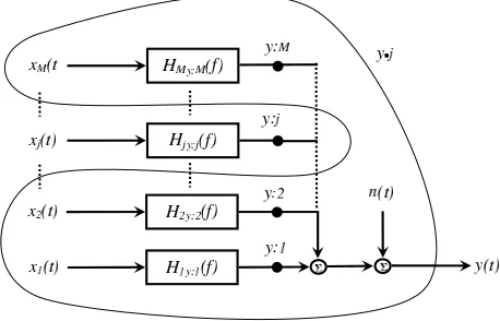
Figure 1. Multiple Source Acoustic Measurement to turn individual sources off without effecting

B. Identification Techniques

Three techniques of source identification are examined in this section and the performance of each evaluated with experimental data. The procedures are all frequency domain methods and depend to some extent on the coherence function. The Coherent Output Power (COP) technique, reported by Halvorsen and Bendat,3 _{requires a measure of at least one input and one output irrespective of the number of inputs.} The Signal Enhancement (SE) technique, developed by Chung,4 _{requires three output measurements for the} identification of a single unmeasured source. The Conditional Spectral Analysis (CSA) technique, proposed by Hsu and Ahuja,1 _{is a combination of these, where one of two inputs is monitored with three output} measurements. A series of tests have been conducted here to examine the procedures for specific aero-engine applications.

1. Coherent Output Power

In real situations extraneous noise may be measured at the input and/or output of a system. Figure 2 shows the general model where u(t) passes through the system to produce the true output v(t). m(t) and n(t) represent the extraneous noise measured within x(t) andy(t). A particular case of interest is where there is no input noise and the output noise is uncorrelated with both the input and output measurements, viz. x(t) =u(t),y(t) =v(t) +n(t) andGxn=Gvn= 0. Given these conditions, the following expressions can be expressed:

Gvv = |Gxv| 2

Gxx =

|Gxy|2

Gxx =Gyyγ

2

xy (1)

Gnn=Gyy−|Gxy|

2

Gxx =Gyy(1−γ

2

xy) (2)

The product Gyyγxy2 , as discussed by Halvorsen and Bendat,3 is called the coherent output spectrum and Gyy(1−γ2xy) is termed the noise output spectrum. This is a highly significant result as we see that the

immeasurable component of y which is attributable to the input xcan be determined from the measured records. We can see, as presented graphically in figure 1, that the coherent output spectrum decomposes the output into one part correlated with the input, and a second uncorrelated with the input,viz., y(t) =

y:j(t) +y·j(t).

The principle limitation of the COP technique is that a measure of one source of interest alone, i.e. a source which is uncorrelated with other inputs to the output measurement, may be difficult to obtain and that it in turn may also contain extraneous noise. When this is the case, the calculated coherent output spectrumGv′v′ may be significantly less than the actualGvv as illustrated in equation (3).

Gv′v′ =γ_x2′yGyy=Gvv

Gxx

Gxx+Gmm ≤Gvv (3)

The techniques of Karchmer56 _{each use theCOP technique to measure the core noise contribution of a} gas turbine or aircraft engine to a farfield measurement.

2. Signal Enhancement

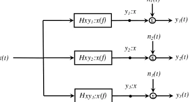
As shown in equation (3), an input measurement which contains noise will result in an erroneously low coherent output spectrum. If the coherence between the input and output is high, one may be confident in the calculated COP. However, if the coherence is low, then it is difficult to establish whether this is due to noise in the output measurement only or whether there is noise present in the input also. Chung4 _developed a technique which can accommodate for the situation as seen in the model in figure 2 if at least three output measurements are available. If three measurements each contain the same correlated source, a new model may be depicted, as in figure 3.

With regard to figure 3, Chung4_{and Bendat and Piersol}7_{demonstrate that the contribution of the input} to each of the outputs can be calculated using only the three output measurements. ForGy2, for example, the following can be derived:

Gy2:x=

|γy1y2||γy2y3|

|γy1y3| Gy2y2 =

|Gy1y2||Gy2y3|

The noise is calculated through subtraction from the total measurement. A typical application of this technique is to remove self-induced flow noise from a microphone measurement. Stoker et al8 _{applied this} technique for separating wind-tunnel background and wind noise from measurements made in the interior of an automobile test in a wind-tunnel.

Figure 2. Input/Output Relationship with

Noise Figure 3. Signal Enhancement Model

3. Conditional Spectral Analysis

One of the limitations of the SE technique is that for measurement locations within the same pressure field, the technique may be applied only when there is a single correlated source between the records. Minami and Ahuja9 _{discuss the errors resulting from using the Signal Enhancement technique when two sources, as} opposed to only one source, are buried within extraneous noise. For the situation where there are only two correlated sources, and a measure of one of them is attainable, the COP and the SE techniques may be used in conjunction with each other and with conditional spectral analysis to successfully identify both sources and the extraneous noise. This approach is presented by Hsu and Ahuja.1

The problem case is illustrated in figure 4(a). The first stage consists of separating out the part correlated with the measurable source, using the COP technique, and thus identifies its contribution. The second stage uses a partial coherence form of the SE technique on the residual to remove the extraneous noise, see figure 4(b). A measure of at least one of only two sources and three output measurements are required for this technique.

(a) Stage 1 using the COP technique (b) Stage 2 using the SE technique on the residual

Figure 4. Conditional Spectral Analysis Technique

C. Experimental Set-up

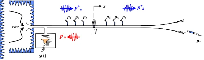
noise as well as reflections. A number of microphones can be located upstream and downstream of the fan, at various axial and circumferential positions, such that they are mounted flush with the inside of the pipe. Additional microphones can be located in the near-field. Also illustrated, is how the electrical signal to the speaker can be recorded with a view to using this signal to condition the measured pressures.

Figure 5. Schematic of Experimental Rig

A 32 channel data acquisition system was used to acquire the data. This consisted of 2 X 16 bit simultaneously sampling Kinetic Systems V200 cards mounted into a National Instruments chassis. A PC running LabView, was used via a National Instruments PCI card to acquire the data from the National Instruments MXI controller card in the chassis. All data, once acquired into time domain files by LabView, were subsequently processed using Matlab.

D. Experimental Results and Evaluation of Techniques

In order to evaluate these three noise source identification techniques for a rotor/stator application, two benchmark test-cases were examined. The first where tonal noise was emitted from the speaker, the second, where band limited broad band noise was convected down the duct;

1. Sine at 1kHz, the fan rotating at 18500 rpm.

2. Broad band noise, high pass filtered at 500Hz, low pass filtered at 3000Hz. The fan rotating at 17250 rpm

The performance of the COP technique is examined using test-case 1 under two sets of circumstances. The first, figure 6 A, is where the measurement at microphone 4, downstream of the fan, is decomposed into a part coherent with the speaker signal and a part which is not (not shown). This is a successful application of the technique when a high signal to noise ratio measurement of a noise source is available. It can be seen that even very low coherence levels of close to zero, result in the coherent output spectrum, e.g. in figure 6 A, maintaining the same qualitative shape. However, it can also be observed that although a peak at the BPF of ≈2500Hz, is present in the spectrum it is two orders of magnitude lower than in the microphone signal. A high number of averages is needed to remove noise from the coherence function.

In figure 6 B, the COP technique is used again but in this instance the upstream microphone 1 is used as the input. For this situation, not only is the convected speaker tone measured at both locations but also the fan BPF and energy related to shaft unbalance. This technique is seen to work effectively here at removing extraneous noise from the downstream measurement which is unrelated to the upstream measurement. Using two upstream microphones and an upstream anechoic termination, the upstream incident signal could have been determined, using the technique of Chung and Blaser,10 _{for example, and this signal compared with} the result of figure 6 A. However, to decompose a signal into incident and reflected waves upstream of a turbine in an aero-engine is challanging.

As discussed in section 2, when noise is present in the input measurement, the COP technique tends to underestimate the coherent contribution. By using a third microphone measurement, the SE technique can be employed to remove the input noise. Figure 6 F shows the new coherence function used in conjunction with microphone 4 when the third microphone 6 is included in the analysis. It can be seen in particular how at the BPF and the speaker tone, noise has been removed resulting in a greater measured contribution.

Figure 6. The performance of COP and the CSA techniques for test case 1. The top row shows the PSD for microphone 4 in blue with the decomposed part of the signal superimposed in red. The bottom row shows the coherence function used in the respective decompositions.

(a) The result using the SE technique at microphone posi-tion 4 using microphones 1, 4 and 6.

(b) The CSA technique is applied using the same three mi-crophones and a measure of the speaker signal.

contribution to be decomposed into two parts. A variation of this technique is available which takes into account noise in the input measurement, an implementation of which can be seen in Bennett and Fitzpatrick.2

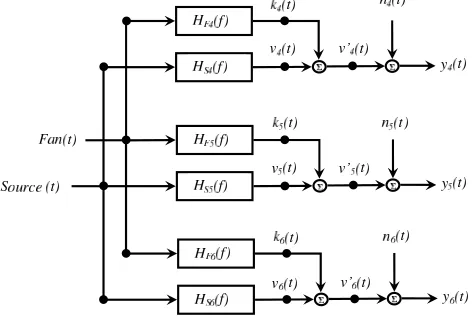
Figure 8. Model assumed for microphones 4, 5, and 6 downstream of the fan, with the fan turned on. Source input, Fan noise input and uncorrelated noise.

For test-case 2, the CSA technique only was used. The model for this case, using only the downstream microphones 4, 5 and 6 is given in figure 8, where the particular equations needed for the decomposition of the microphone 5 measurement are given by

Gv5v5 =Gy5y5:s=

|Gsy5|2

Gss

Gk5k5 =|γy4y5·s||γy5y6·s|

|γy4y6_·s|

Gy5y5·s

Gn5n5 = 1−|γy4y5·s||γy5y6·s|

|γy4y6_·s|

!

Gy5y5_·s

(5)

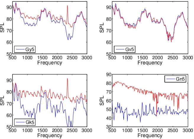
For test-case 2, the results of the decomposition are presented in figure 9. In this experiment the plots in blue are the results for microphone 5 before the fan is turned on. Gy5 is the total energy as measured by microphone 5. Gv5 is the part of this measurement coherent with the speaker, i.e. the broad band noise. Gn, in the absence of the fan being turned on, is low and more attributable to electrical noise and instrumentation characteristics than any acoustic phenomenon. Gk5, is seen, in blue, to have similar qualitative characteristics to the identified Gv5 component. This is due to background noise in the lab exciting the duct frequencies in a similar fashion to the speaker, albeit at a far lower magnitude.

When the fan is turned on, the plots in red show the additional noise measured and identified. The energy at microphone 5, Gy5, increases at the BPF and also across the frequency range. The speaker signal remaining constant, Gv5 is seen to be accurately identified. The noise signal, Gn5, has greatly increased, markedly so at the lower frequencies, and being incoherent with the other microphone signals, is most likely to be hydrodynamic noise. The Gk5 signal alone contains the BPF signal. The smaller peaks are duct frequencies which in the presence of flow, are convected along the duct and are thus measured at all microphone locations. These peaks are to be seen also in the blue plot but are seen to decrease in some frequency ranges. Due to the length and end conditions of the duct, the microphones will be located close to nodes of some modes which are thus measured with a low magnitude. The convection is seen to result in energy at these frequencies being measured all all locations.

III.

Non-linear Analysis

A. Introduction

Figure 9. For microphone 5 only, the results of the identification using the CSA technique with and without the fan turned on. The broad band noise test-case 2 was examined here.

between combustion noise measurements made at the combustor can with pressure transducers, and micro-phone array measurements focused on the exit plane of an aero-engine, when the rpm of the engine was increased, was reported by Siller et al.11 _{An interpretation of this result is that, when the jet noise is low} for low engine power settings, the core noise is a significant contributor to noise in the near-field. However, as the jet noise becomes more significant, the coherence drops due to the relatively low contribution of the combustion noise. This rationale assumes a linear frequency response function between the combustion can and the exit plane of the engine. It is also possible that the reduction in coherence is due to some non-linear interactions as the unsteady pressure from the combustor passes through the rotor/stator stages. For the situation where the combustion noise is acted upon in a non-linear fashion, as illustrated schematically in figure 10, the identified contribution will be inaccurate. This paper also examines the scenario where a fluctuating pressure is modified, in anon-linear sense, as it is convected through a rotating vane-axial fan.

Interaction between rotors is a common observation in turbo-machinery noise and has been discussed analytically by Cumpsty,12_{Holste and Neise,}13 _{Enghardt et al.}14 _{and numerically by Nallasamy.}15 _Energy at two different frequencies may interact to induce energy at a third. In these situations, the upstream energy source is a rotor-stator pair whose excited spinning modes impinge upon a second rotor. The case where broad band or narrow band noise, such as may originate from a combustor, interacts with a rotor-stator pair, (e.g. turbine noise), producing noise at sum and difference frequencies is explored in this paper. This requires further analysis to determine the process, but is thought to be analogous with the theories reported Cumpsty12 _{and Moore,}16 _{i.e., the combustor mode can be viewed as a inflow-distortion interacting with the} rotor.

The non-linear analysis of this paper investigates, with reference to figure 10, how to accommodate, in addition to convected combustion noise and turbine noise being measured at the exit plane of an aero-engine,

Figure 10. Schematic of an aero-engine where pressure measurements are taken at the combustion can and at the exit plane.

Figure 11. Frequency response function between the combustion noise and the pressure measured at the exit plane when some rpm dependent non-linearity is included in the model.

B. Non-linear Simulations

In order to investigate this, a series of simulations were performed using synthetic data. When a signal is operated upon by a non-linear system, its frequency components are modified. Common interactions are quadratic in nature resulting in sum and difference frequencies as well a doubling in frequency. This can be demonstrated by observing the following two trigonometric identities.

[Acos(ωt)]2=1 2A

2_{[1 + cos(2ωt)] (6)}

[Acos(ω1t) +Bcos(ω2t)]2= 1 2A

2_{[1 + cos(2ω} 1t)] +

1 2B

2_{[1 + cos(2ω}

2t)] +ABcos(ω1+ω2)t+ABcos(ω1−ω2)t (7)

The doubling of frequency arises from self interaction, whereas the sum and difference frequencies come about from combination interactions.

(a) Incident pressure upstream (b) Incident pressure downstream

Figure 12. Incident pressure models accommodating a quadratic non-linear term.

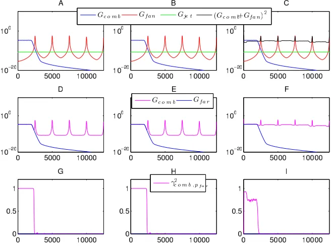
where the filter used was a Butterworth IIR filter. Figure 13(A) shows the basic simulation. In addition to the input terms of figure 12, the exit plane measurement of an aero-engine is simulated to contain broad band jet noise in green. Tonal fan (turbine) noise is shown in red and low frequency band limited combustion noise in blue. Plots (B), (E) and (H) in figure 13 are identical to (A), (D) and (G) in this figure. Figure 13(C) shows the non-linear quadratic input (Gcomb+Gf an)2_{in addition to the others. A point to be noticed} here, is how due to the frequency interactions, significant energy is created at frequencies where the linear terms’ energy is quite low. Row 2 of this figure shows the sum of the components, in magenta, representing an exit plane measurement, and the combustion noise only in blue, representing an upstream measurement. Row 3 plots the coherence between these latter two, i.e. the combustion noise and the total noise. It is shown how for thislow power case, the coherence is quite high.

Figure 13. Combustion Noise, Fan Noise and Jet Noise simulation at a low power setting. Column 1 and column 2 are linear and are identical here. Column 3 contains a non-linear quadratic interaction term.

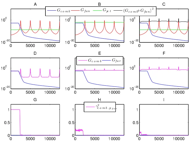
Figure 14, plots the same information for thehigh power case. In column one all three inputs increase by the same amount resulting in no change to the coherence. In column 2, the fan noise and combustion noise increase by the same amount as in column 1, but the jet noise increases by relatively more. The coherence is seen to drop here, due to the relative decrease in contribution of the combustion noise to the total noise. This is the “linear” interpretation of the data presented in Siller et al.11 _{Column three shows the same} increase in power of the three linear terms as in column 1 but in this case, due to the non-linear nature of the quadratic term, it increases relatively more, causing it to dominate, which results in the drop in coherence. It is therefore the presence of the non-linearity that causes the drop in coherence and not a decrease in the combustion noise relative to the other linear terms.

Figure 14. Combustion Noise, Fan Noise and Jet Noise simulation at ahigh power setting. In column 1, all three components have been increased by the same amount. In column 2, combustion and fan noise have been increased the same a mount as column 1 but jet noise by relatively more. In column 3, the linear inputs are increased the same amount as in column 1.

noise reduction in the presence of a non-linear interaction, but also how important it is to be able to identify the non-linear process as incorrect deductions can be made without knowledge of its presence.

A second set of simulations were performed with narrow band noise, for the combustor instead of the low frequency band limited noise used in the previous simulations. Jet noise is omitted from these simulations to simplify the analysis. It can be seen readily in figure 16(B) how the non-linear term is made up of double frequencies as well as sum and difference tones.

Thus, it can be seen that with this data, if the COP technique was used between the combustion noise only and the total noise, then the only contribution to the total noise made by the combustor would be identified as being low frequency narrow band noise. For a non-linear process this would be an incorrect deduction, however, as the combustor also contributes to the total noise at all the higher interaction frequencies too. Without close inspection and measurement, the higher interaction frequencies could be mis-interpreted as rotor-stator interaction noise, particularly for aero-engines with many blades and vanes over many stages.

C. Investigation Above Plane Wave Region

An analysis was performed on the experimental rig of section II to detect the presence of non-linearities. However, in order to investigate this hypothesis that convected upstream noise might interact with a ro-tor/stator pair to produce acoustic energy at sum and difference frequencies, the experimental investigation had to be extended above the plane wave frequency region.

While varying the amplitude and frequency content of the speaker signal, the PSD of a microphone located downstream of the fan was examined. A set of tests was carried out where the speaker tone was incremented in steps of 500Hz or 250Hz, from 500Hzto 12.5kHz. A waterfall plot of these results is shown in figure 17. The first averaged PSD in this plot is for the fan-only turned on. With each successive test, the frequency from the speaker is increased. This plot is revealing, as there is no indication of non-linear interaction until the speaker frequency reaches 8.75kHz, above which only a sum tone is detectable. In addition, according to the model of figure 12(b), difference frequencies with higher BPF harmonics should be measurable. Figure 18 plots the expected interactions for an upstream tone of 9.3kHz assuming a quadratic model. To help understand the reason for these anomalies, the cut-on frequencies for the higher modes in the duct were superimposed onto the waterfall plot. It can be seen clearly how the interaction tone appears only above

Figure 15. Comparison of the two scenarios. The total exit plane pressure is similar in both cases. However, in the first case Jet Noise dominates whilst in the second case it is the non-linear term which is greatest.

Figure 17. For microphone 5 only, the results of the identification with and without the fan turned on.

therefore, that the non-linear term [Comb(t) +F an(t)]2_{plotted in figure 18, needs to be used in conjunction} with duct modal theory. That is to say, if energy at two frequencies interact to create energy at a third, then this energy will only propagate down the duct if the mode which carries it is above its cut-on frequency.

0 2000 4000 6000 8000 10000 12000 10−20

10−15 10−10 10−5 100 105

Frequency [Hz]

PSD

Gfan Gcomb ustor [Gfan +Gcomb ustor]2

Figure 18. Simulated data representing a quadratic interaction between the fan and combustor, with a BPF of 2400Hz and a combustor frequency of 9.3kHz.

Based on this idea, it is posited that the interaction tone has a modal structure of either (+4,0), (−4,0), (+1,1) or (−1,1), or possibly some combination of these. In addition, this modal structure comes about as a result of the interaction of the modal structure of the BPF frequency with that of the speaker fre-quency.

It has been shown experimentally that acoustic energy in a duct at a certain frequency may interact with fan noise at a different frequency to scatter energy to a third frequency which is a sum of the two. This would appear to support the model suggested in figure 11, but as discussed above, the proposal that the process is a non-linear quadratic interaction, figure 18, is only partially verified. In order to understand why the sum interaction only seems to occur above the cut-on frequency of certain higher-order modes, it would be useful to perform a modal decomposition of the pressure field upstream and downstream of the fan in order to determine the modal content of the incident tone and the sum tone.

D. Non-Linear Identification Techniques

alone is readily available. The model of figure 19 represents the physical situation in the duct. In the figure, the two principle acoustic inputs into the duct, which are indicated in red, are the combustion noise and the fan noise. In green, x(t) is an upstream measurement, whereas y(t) is a measurement downstream of the fan. The downstream measurement, y(t), will always contain the sum of the linear parts in addition the the non-linear component, when present, whereas the upstream measurement, x(t), will be comprised of the source noise as well as the fan noise and the non-linear contribution (when present) depending on the conditions for back propagation. As a consequence of this, the model of figure 19 can be simplified to figure 20, where the second, non-linear, component is included when the physics dictates. An example can be given with reference to figure 17, where the downstream measurement, in this case, is linear until the speaker signal is raised above 8.75kHz, when the second, non-linear term needs to be included. The difficulty therefore, is to separate the non-linear part from the linear part when the non-linear part is present.

The model presented in figure 21 facilitates this linear/non-linear decomposition, when the underlying non-linear phenomenon is quadratic in nature. Squaring the input x(t) results in the following expansion

(C+F) + (C+F)22

=C2+ 2CF+F2+6C2F+6CF2+4C3F+6C2F2+4CF3+2C3+2F3+C4+F4 (8)

when the non-linear component is present. As can be seen from the right-hand-side; the first three terms are the expansion of the non-linear part whereas the linear parts, i.e., C and T, do not appear. Therefore a coherence between the square of the input with the output should isolate the non-linear part of the output only. This technique was applied to the data presented in section C and is shown in figure 22. As can be seen, the coherence is ≈ 0 apart from at the interaction tones above 11200Hz, and at some of the nBPF frequencies. In addition, some interaction is seen to take place between the shaft imbalance and the nBPF frequencies, with some sum and difference frequencies around the nBPF frequencies identified. The non-linear identification at the nBPF frequencies may be a result of the amplitude of the BPF being of sufficiently high amplitude to have become acoustically non-linear in itself. For such situations, the linear approximation of the wave equation is no longer valid and the higher order terms become significant. It should be noted that as acoustic pressure increases, the first non-linear terms of the wave equation to become significant are quadratic.

In addition to the isolation of the non-linear contribution, using the model of figure 21, the technique of Rice and Fitzpatrick,17 _{allows the non-linear part to be removed from the input and output. The required} partial coherence function, defined by

γij2·r=

|Gij·r| 2

Gii_·rGjj_·r

(9)

where

Gij_·r=Gij− GirGrj

Grr (10)

and

Gii_·r=Gii−

|Gri|2

Grr (11)

when applied, results in the input conditioned on the square of the input, i.e. the linear contribution.

Figure 20. Inputs into upstream and down-stream measurements can be modelled as hav-ing linear and non-linear parts.

Figure 21. Inputs into upstream and down-stream measurements can be modelled as hav-ing linear and non-linear parts.

0 2000 4000 6000 8000 10000 12000

0 1000 2000 3000 4000 5000 6000 7000 8000 9000 10000 11000 12000

0 0.5 1

Test Point γ_{m 1}2 2₋m 5

Frequency [Hz] Coherence

IV.

Full Scale Engine Tests

A. Introduction

The non-linear identification techniques, developed with the experimental rig, were applied to data from full scale turbo-fan engine tests. A Rolls-Royce engine was instrumented with pressure transducers at the combustor can and in the hot jet pipe, and microphones were placed in the near-field. A schematic of some of the instrumentation is shown in figure 23. The results from five steady-state points (engine power settings), were examined. The power settings defined for the test included some diagnostic conditions that are not necessarily representative of operational conditions.

For the highest of the five test points, the PSD of the hot-jet pipe transducer,RPB, is shown in figure 24. A number of interesting points can be noted in this figure. Firstly, a tone in the combustor can is generated at ≈500Hz. This tone is of sufficiently high amplitude as to generate superharmioncs. The tone and the superharmonics are measurable downstream of the turbine. Secondly, a tone generated from rotor/stator interaction in the high pressure turbine is measurable downstream of the turbine near the exit plane. Thirdly, the combustion tone and its superharmonics interact with this HPT tone in a non-linear fashion similar to that observed with the experimental rig: sum and difference frequencies are formed due to combustion noise impinging on a rotor/stator pair. It is most significant, that not only does this interaction occur, but that the interaction tones along with the HPT tone and the combustor tones are able to propagate through the circuitous path created by the various stages of the turbine.

Figure 23. Engine Instrumentation schematic with location of external farfield microphone.

Figure 24. PSD at sensor location in the hot-jet pipe (RPB) for a particular engine power. A combustor tone at ≈500 Hz is measured as well as superhar-monics. A HPT tone, convected through the turbine is also measured. To be seen on either side of this tone is energy at sum and difference frequencies.

B. Non-linear Analysis

Lowest Highest

0 0.5 1

Engine Order - N3 γ2

R P 1−R P B

Test Point Coherence

1HPT1 Sum and Difference

Combustor Tones

Figure 25. The coherence between the combustion can sensor RP1 and the hot-jet pipe sensor RPB for five increasing power test points.

Lowest Highest

0 0.5 1

Engine Order - N3 γ2

(R P 12₎ −R P B

Test Point Coherence

In addition to being a tool for non-linear interaction identification, this quadratic analysis approach can be used, as explained in section D, to separate the non-linear contribution to the spectrum from the linear part. The model of figure 21 was used and the full scale test data processed with the following equations;

Non−linear COP =γ₍2RP12_{,RP B)}G_{(RP B,RP B)} (12)

Linear COP =γ₍2_{RP1,RP B)}

·RP12 G(RP B,RP B)·RP12 (13)

Figure 27 shows the standard COP calculated between the combustor can location and the hot-jet pipe location. This coherence function of plot B, in conjunction with the COP in red in figure A, would be used, for example, to assess the frequency range for which acoustic treatment might be designed to reduce combustion noise radiation to the farfield. However, as figure 28 displays, the frequency range that the non-linear contribution spans is far greater than that attributable to the actual sound source, as plotted in figure 29. As it is difficult to design acoustic treatment to absorb sound over a large frequency range, the ability to identify the non-linear contribution means that efforts can be divided into two parts; a). absorption or reduction of the (linear) combustion noise, ideally upstream of the turbine, and, b). tackling the non-linear interaction process separately. Obviously, if the combustion noise is reduced upstream of the turbine, then, as highlighted in the simulations, the contribution of the non-linear noise is greatly diminished.

This analysis was applied to the frequency range around the 1HPT1 tone also, and successfully identified the sum and difference tones as well as subtracting them from the COP, decomposing it into linear and non-linear parts.

It should be noted that the combustor tone and harmonics were seen to interact with the LPT also, causing sum and difference frequencies to be generated.

0 500 1000 1500 2000 2500 3000 3500 4000 xdB

(x+20)dB

(A)

Frequency, Hz

0 500 1000 1500 2000 2500 3000 3500 4000 0

0.5 1

(B)

Frequency, Hz

Coherence

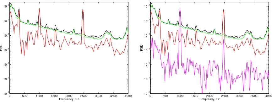
Figure 27. Plot B shows the coherence between the combustion can sensor RP1 and the hot-jet pipe sensor RPB. Only the frequency range 0-4kHz is displayed. In plot A, the PSD of RPB, in blue, is compared to the coherent output power using the coherence of plot B.

V.

Conclusions

0 500 1000 1500 2000 2500 3000 3500 4000 xdB

(x+20)dB

(A)

Frequency, Hz

0 500 1000 1500 2000 2500 3000 3500 4000 0 0.5 1 (B) Frequency, Hz Coherence

Figure 28. The non-linear part of the COP is plotted versus the PSD of RPB

0 500 1000 1500 2000 2500 3000 3500 4000 xdB

(x+20)dB

(A)

Frequency, Hz

0 500 1000 1500 2000 2500 3000 3500 4000 0 0.5 1 (B) Frequency, Hz Coherence

Figure 29. The linear part of the COP is plot-ted versus the PSD of RPB

experimental technique was developed which enabled the non-linear interaction between the convected sound source with the vane-axial fan to be detected and identified when present. The technique was extended to allow the linear and non-linear acoustic contributions to be separated. From analysis of data from full scale turbo-fan engine tests frequency scattering was seen to occur between the combustion noise and the high pressure turbine which was measurable in the hot jet pipe after convection through the many turbine stages. The techniques allowed the non-linear interaction to be successfully identified and linear and non-linear coherent output powers to be determined.

Acknowledgements

This work was partly supported by the SILENCE(R) project which is funded under EU Commission contract no. G4RD-CT-2001-00500

References

1

Hsu, J. S. and Ahuja, K. K., “A coherence-based technique to separate ejector internal mixing noise from farfield measurements,”AIAA/CEAS 4th Aeroacoustics Conference, No. AIAA-98-2296, June 2-4 1998.

2

Bennett, G. J. and Fitzpatrick, J. A., “A comparison of coherence based acoustic source identification techniques,”12th International congress on sound and vibration, No. 950, Lisbon, Portugal, 11-14 July 2005.

3

Halvorsen, W. G. and Bendat, J. S., “Noise Source Identification Using Coherent Output Power Spectra,”Sound and Vibration, Vol. 9, No. 8, 1975, pp. 15, 18–24.

4

Chung, J. Y., “Rejection of flow noise using a coherence function method,”J. Acoust. Soc. Am., Vol. 62, No. 2, 1977, pp. 388–395.

5

Karchmer, A. M., Reshotko, M., and Montegani, F. J., “Measurement of far field combustion noise from a turbofan engine using coherence function,”AIAA 4th Aeroacoustics Conference, No. AIAA-77-1277, Atlanta, Georgia, October 3-5 1977.

6

Karchmer, A. M., “Conditioned pressure spectra and coherence measurements in the core of a turbofan engine,” Tech. Rep. TM82688, NASA, 1981, AIAA Paper 81-2052.

7

Bendat, J. S. and Piersol, A. G.,Random Data: Analysis and Measurement Procedures, John Wiley & Sons, 1986.

8

Stoker, R. W., Ahuja, K. K., and Hsu, J. S., “Separation of Wind-Tunnel Background Noise and Wind Noise from Interior Measurements,”AIAA/CEAS 2nd Aeroacoustics Conference, No. AIAA-96-1763, Palo Alto, May 6-8 1996.

9

Minami, T. and Ahuja, K. K., “Five-microphone method for separating two different correlated noise sources from farfield measurements contaminated by extraneous noise,” AIAA/CEAS 9th Aeroacoustics Conference, No. AIAA-03-3261, South Carolina, May 12-14 2003.

10

Chung, J. Y. and Blaser, D. A., “Transfer Function Method of Measuring In-Duct Acoustic Properties. I. Theory.”J. Acoust. Soc. Am., Vol. 68, No. 3, 1980, pp. 907–913.

11

Siller, H. A., Arnold, F., and Michel, U., “Investigation of Aero-Engine Core-Noise Using a Phased Microphone Array,”

7th AIAA/CEAS Aeroacoustics Conference, No. AIAA-2001-2269, Maastricht, The Netherlands, 28-30 May 2001.

12

Cumpsty, N. A., “Sum and difference tones from turbomachines,”Journal of Sound and Vibration, Vol. 32, No. 3, 1974, pp. 383–386.

13

Holste, F. and Neise, W., “Noise Source Identification in a Propfan Model by Means of Acoustical Near Field Measure-ments,”Journal of Sound and Vibration, Vol. 203, No. 4, 1997, pp. 641–665.

14

mode analysis using in-duct sensor rakes,”7th AIAA/CEAS Conference on Aeroacoustics., No. AIAA-2001-2153, Maastrict, The Netherlands., May 2001.

15

Nallasamy, M., Hixon, R., Sawyer, S., Dyson, R., and Koch, L., “A Time Domain Analysis of Gust-Cascade Interaction Noise,”9th AIAA/CEAS Aeroacoustics Conference and Exhibit, No. AIAA-2003-3134, Hilton Head, South Carolina, May 12-14 2003.

16

Moore, C. J., “In-duct investigation of subsonic fan “rotor-alone” noise.”J. Acoust. Soc. Am., Vol. 51, 1972, pp. 1471– 1482.

17