Conjugate Gradient Method to Solve Fluid Structure Interaction Problem

(1)

http://www.scirp.org/journal/am ISSN Online: 2152-7393

ISSN Print: 2152-7385

Conjugate Gradient Method to Solve Fluid

Structure Interaction Problem

Mamadou Diop

1

, Ibrahima Mbaye

2

1_{Thies University, Thies, Senegal}

2_{Department of Mathematics and Computer Science, Thies University, Thies, Senegal}

Abstract

In this paper, we propose a method to solve coupled problem. Our computa-tional method is mainly based on conjugate gradient algorithm. We use finite difference method for the structure and finite element method for the fluid. Conjugate gradient method gives suitable numerical results according to some papers.

Keywords

Fluid-Structure Interaction, Beam, Stokes, Finite Element, Finite Difference Method, Conjugate Gradient Method

1. Introduction

Problem involving fluid structure interaction occurs in a wide vatiety of engineering problems and therefore has attracted the interest of many investiga- tions from different engineering disciplines. As a result, much efforts has gone into the development of general computational method for fluid structure sys-tems [1] [2] [3] [4] [5] [6].

Amongst the computational methods for fluid structure interaction problem, we cite the fixed point method, the Newton method, the Quasi-Newton method, the fictitious domain method. In this work we present a method based on the conjugate gradient algorithm. In effect, the fluid interaction problems occur in biomedical fluids areas for example blood flow interaction with elastic veins. Thus, this paper aims at showing that, we can combine the finite difference me-thod, the finite element method and the conjugate gradient method to solve fluid structure interaction problem. On the one hand, we use finite difference method to approximate the structure model in order to have a linear systems, On the other hand, we solve the stokes equation by the finite element method. Moreover,

How to cite this paper: Diop, M. and Mbaye, I. (2017) Conjugate Gradient Me-thod to Solve Fluid Structure Interaction Problem. Applied Mathematics, 8, 444-452. https://doi.org/10.4236/am.2017.84036

Received: February 18, 2017 Accepted: April 21, 2017 Published: April 24, 2017

http://creativecommons.org/licenses/by/4.0/

(2)

conjugate gradient method will be intruduced to compute the displacement of the structure. Thus, the velocity v and the pressure p of the fluid are done in

the deformed domain. In addition, the fluid represented by the blood is mod-elled by two dimensional Stokes equation for steady flow and the structure represented by the body vessel is modelled by the one dimensional beam equa-tion.

2. Position of Problem

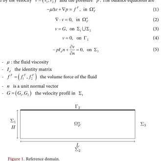
2.1. Domain Fluid

The fluid domain noted u 2

F

Ω ⊂ is represented in the Figure 1. Where, the border 1 2 3 2

u F

∂Ω = Σ Σ Σ Γ .

- Γ2 is the interface between the fluid and the elastic structure

- Σ1 is The inflow

- Σ2 is a rigid border

- Σ3 is the outflow

- L is the domain length

- H is the domain height

- u is the displacement of the structure

2.2. Fluid Properties

The fluid is considered to be Newtonian, incompressible and its state is describ- ed by the velocity v=

(

v v1, 2

)

and the pressure p. The balance equations are

, in

F u

F

v p f

µ

− ∆ + ∇ = Ω ₍₁₎

0, in uF v

∇ ⋅ = Ω (2)

1 2

, on

v=G Σ Σ (3)

2 0, on

v= Γ (4)

3

0, on

d

v pI n

n

∂

− + = Σ

∂ (5)

-

µ

_{: the fluid viscosity}

- Id the identity matrix

-

(

1 , 2

)

F F F

f = f f the volume force of the fluid

- n is a unit normal vector

[image:2.595.213.543.403.733.2]

- G=

(

G G1, 2

)

the velocity profil in Σ1

(3)

2.3. Structure Properties

The structure is assumed by elastic beam. We note u: 0,

[ ]

L → the displace-

ment of the structure, it is modelled by the beam equation

( )4

_{( )}

₍

_{( )}

₎

_{[ ]}

, , 0, ,

Du x = p x H+u x ∀ ∈x L (6)

with the boundary conditions,

( )

0

( )

0

u =u L = (7)

( )

0

( )

0

u′ =u L′ = (8)

where,

•

₍

3₂

₎

12 1 E h D

ν

× = −

• E is the Young modulus

• h elastic structure thickness

• ν _{the Poisson's coefficient}

Remark: In Equation (6) we assume that only the pressure force is acting on the interface and also u is the transversal displacement [3].

3. Coupled Problem

The coupled problem is to find

(

u v p, ,

)

such that:

( )

_{( )}

₍

_{( )}

₎

_{[ ]}

( )

4 1 2 2 3 , 0, 0 0 0 0

, in 0, in

, on 0, on

0, on

F u

F

d

Du x p x H u x x L u u L

u u L v p f v v G v v pI n n µ  = + ∀ ∈  = =   ′ = ′ = 

− ∆ + ∇ = Ω 

∇⋅ = Ω 

= Σ Σ



 = Γ



∂

− + = Σ

 _∂





In order to solve this coupled problem, we transform its continuous problem into a discreet problem by using finite difference method and finite element method.

3.1. Approximation by Taylor Development

Assumption: We consider u as a small displacement.

Thus, the Taylor formula gives

( )

(

)

(

) ( ) (

,

)

, , p x H ,

p x H u x p x H u x

y

∂

+ ≈ +

∂ (9)

the Equation (6) becomes:

( )4

_{( ) ( ) (}

,

)

₍

₎

, ,

p x H

Du x u x p x H

y

∂

− =

∂ (10)

we pose

( )

x p x H

(

,

)

y

α = −∂

(4)

( )4

_{( )}

_{( ) ( )}

₍

₎

, .

Du x +

α

x u x = p x H (11)

To discretize the Equation (11), we introduce a space step

1

L x

N

∆ =

+ . We

denote by ui the value of the discrete solution at xi= × ∆i x for i∈

{

0,1,,N+1

}

.

We must also discretize The boundary conditions . A centred formula gives

1 1 et N 2 N

u =u− u + =u (12)

and the boundary conditions u

( )

0 =u L

( )

=0 become

0 N 1 0

u =u + = (13)

we rewrite the Equation (11) in the discreet form

(

)

2 1 1 2

4

4 6 4

, 1, 2, 3

i i i i i

i i i

u u u u u

D u P x H i N

x α

− − − + − + + + ₊ ₌ ₌

∆  (14)

Then, the continuous problem becomes the following algebraic equation

AU =P, where

1

4 4 4

2

4 4 4 4

3

4 4 4 4 4

2

4 4 4 4 4

1

4 4 4 4

4 4 4

7 4

0 0 0

4 6 4

0 0

4 6 4

0

4 6 4

0

4 6 4

0 0

4 7

0 0 0

N

D D D

x x x

D D D D

x x x x

D D D D

x x x x x

A

D D D D D

x x x x x

D D D D

x x x x

D D D

x x x

α α α α α α − − −  ₊  _∆ _∆ _∆    − −  ₊   _∆ _∆ _∆ _∆   ₋ ₋   ₊   ∆ ∆ ∆ ∆ ∆    =    − ₊ −  _∆ _∆ _∆ _∆ _∆  − −  ₊  _∆ _∆ _∆ _∆  −  ₊  _∆ _∆ _∆                      

(

)

(

)

(

)

1 1 2 2 , , et , _N N u p x H

u p x H

P U

u p x H

            =_ _ =         _ _    

Proposition 1. Note that A is symmetric positive definite under this

as-sumption

α

( )

x ≥0.

Proof. We will prove that

α

( )

x ≥0 for all x∈

[ ]

0,L .

For all

( )

x y, ∈

[ ] [

0,L × 0,H

]

we have

( )

2

( )

2

( )

,

, ,

F p x y

f x y v x y

y

∂

= + ∆

∂ , for

y=H and x∈

[ ]

0,L we have v2

(

x H,

)

=0, then

(

)

₍

₎

2 ,

,

F p x H

f x H

y

∂

=

∂ . By

choosing 2

(

,

)

s

f x H = − ×g ρ ×h [3] where g is the gravity force and

ρ

s

the structure density, we obtain p x H

(

,

)

0

y

∂

≤

∂ . Finally, we deduce

α

( )

x ≥0

(5)

3.2. Coupled Approximate Problem

Since A is symmetric positive definite, so we can use the conjugate gradient

method to solve the following coupled problem. Find

(

)

(

1

( )

)

2 2

( )

0

, uF uF

v p ∈ H Ω ×L Ω

and U so that

( )

(

( )

)

( )

2 1 0 2

: d div d d ,

div d 0,

u u u

F F F

u F F u F u F AU P

v w x p v x f w x w H

v q x q L

µ

Ω Ω Ω

Ω

 ₌ 

 _{∇ ∇} ₋ ₌ _{∀ ∈} _Ω

 

 = ∀ ∈ Ω



∫

4. Numerical Method

To solve numerically the coupled problem we use the following conjugate gra-dient algorithm.

Proposition 2. Let A be a symmetric positive definite matrix, and u0∈.

Let

(

u r z_k, ,_k _k

)

be three sequences defined by the induction relations

0 0 0

z = = −r P Au , and for

1

1 1

0

k k k k

u u z

k r r Az

z r z

λ λ α + + + + = +   ≥ _ = −  ₌ ₊  with

(

)

2 2 1

2 and

, k k k k k k k r r z Az r

α ₌ + λ ₌

Then,

( )

uk 0≤ ≤ +k k₀1 is the sequence of approximate solutions of the the

conju-gate gradient method [7].

Description of the computational method

Step 1: It computes in the initial field the velocity and the pressure.

Step 2: It uses the conjugate gradient algorithm to find the structure deforma-tion u.

Step 3: It computes again the pressure and the velocity in the deformed do-main

5. Numerical Results

Let the real noted test defined by 2

test= P ×

ε

. We define the stopping

crite-rion of iterations for the conjugate gradient algorithm by rhoold>test and

k<n where, k the number of iterations and rhoold= z0 2.

We assume that the velocity on the boundary fluid domain is [3]:

(

)

(

)

(

)

(

)

(

)

(

)

2 2

1 1 2 1 2 1 2 2 1

1 1 2 1 2 1 2 2 2

1 1 2 1 2 1 2 2 3

, 30 1 and , 0, on

, 30 on , 0, on

, 0 and , 0, on

x

G x x v G x x v

H

G G x x v G x x v

G x x v G x x v

  

= = − = = Σ

  

 

 

= = = = = Σ

 _{= =} ₌ ₌ _Σ

 

(6)

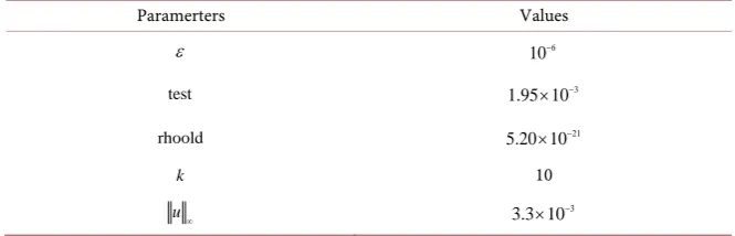
The Table 3 shows that, if we take the tolerance 3

test=1.95 10× − we have the

con-vergence of the algorithm after k=10 iterations and 21

rhoold=5.20 10× − <test and

the norm of the displacement is 3

3.3 10

u_∞ = × − .

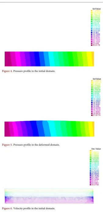
Freefem ++ [8] is used for the numerical tests. Figures 2-7 following display the structure displacement, the pressure and the velocity.

Figure 2. Initial grid.

[image:6.595.212.541.358.451.2]

Figure 3. Final grid.

Table 1. Parameters of the strcuture.

Paramerters Values

E 0.75 10 g cm× 6 2⋅s2

h 0.1 cm

ν 0.3

s

ρ 3

g 1.1

[image:6.595.209.536.484.592.2]

cm

Table 2. Parameters of the fluid.

Paramerters Values

µ g

0.035

L 3 cm

H 0.5 cm

g

2

cm 9.81

s

(

1 , 2

)

F F F

f = f f

(

0, s

)

g ρ h

[image:6.595.207.540.626.733.2]

− × ×

Table 3. Results related to the algorithm.

Paramerters Values

ε ₁₀−6

test _{1.95 10}_× −3

rhoold 21

5.20 10× −

k 10

u_∞ 3

(7)

[image:7.595.200.539.50.742.2]

Figure 4. Pressure profile in the initial domain.

Figure 5. Pressure profile in the deformed domain.

(8)

Figure 7. Velocity profile in the deformed domain.

6. Conclusion

In this paper, we present a method to solve a steady coupled problem. Our me-thod is based namely on the conjugate gradient algorithm, it takes simulta- neously into account three unknown parameters so that each of them depends on the others. To get the results it is necessary to solve the fluid in the initial domain with the finite element method in order to determine the displacement of the structure by the conjugate gradient method and finally to deduce the ve-locity and the pressure. The veve-locity, the pressure and the displacement profile compared to [2] [3] [5] appear good. In this work, the only thing to skill is to reduce the number of iterations and to apply this strategy on the unsteady prob-lem.

References

[1] Mbaye, I. (2012) Fourier Series Development Resulting from an Unsteady Coupled Problem. International Journal of Contemporary Mathematical Sciences, 7, 1695- 1706.

[2] Mbaye, I. (2013) Fourier Series Development for Solving a Steady Fluid Structure Interaction Problem. International Journal of Contemporary Mathematical Sciences, 8, 75-84. https://doi.org/10.12988/ijcms.2013.13008

[3] Murea, C.M. (2005) The BFGS Algorithm for Nonlinear Least Squares Problem Arising from Blood Flow in Arteries. Computers & Mathematics with Applications, 49, 171-186.

[4] Mbaye, I. and Murea, C. (2007) Numerical Procedure with Analytic Derivative for Unsteady Fluid-Structure Interaction. Communications in Numerical Methods in Engineering, 24, 1257-1275.https://doi.org/10.1002/cnm.1031

[5] Mbaye, I. (2012) Controllability Approach for a Fluid Structure Interaction Prob-lem. Applied Mathematics, 3, 213-216.https://doi.org/10.4236/am.2012.33034 [6] Turek, S. and Hron, J. (2006) Proposal for Numerical Benchmarking of

Flu-id-Structure Interaction between an Elastic Object and Laminar Incompressible Flow. Computational Science and Engineering, 53, 371-385.

(9)

Ma-thematical Modelling and Numerical Simulation. Oxford University Press Inc., New York.

[8] Hecht, F. and Pironneau, O. (2003) A Finite Element Software for PDE: Free-Fem++. www.freefem.org

Submit or recommend next manuscript to SCIRP and we will provide best service for you:

Accepting pre-submission inquiries through Email, Facebook, LinkedIn, Twitter, etc. A wide selection of journals (inclusive of 9 subjects, more than 200 journals)

Providing 24-hour high-quality service User-friendly online submission system Fair and swift peer-review system

Efficient typesetting and proofreading procedure

Display of the result of downloads and visits, as well as the number of cited articles Maximum dissemination of your research work

Submit your manuscript at: http://papersubmission.scirp.org/