Discrimination and Estimation of the Maximum Cost Performance of Proton Exchange Membrane Fuel Cell Power Generation with Seven Constants

Discrimination and Estimation of the Maximum Cost

Performance of Proton Exchange Membrane Fuel Cell

Power Generation with Seven Constants

H. F. Zhang, P. C. Pei

State Key Laboratory of Automotive Safety and Energy, Tsinghua University, Beijing, China Email: [email protected], [email protected]

Received January 31, 2013; revised February 28, 2013; accepted March 15, 2013

Copyright © 2013 H. F. Zhang, P. C. Pei. This is an open access article distributed under the Creative Commons Attribution License, which permits unrestricted use, distribution, and reproduction in any medium, provided the original work is properly cited.

ABSTRACT

This paper is dedicated to analytical expression of the maximum electricity-cost ratio (M-ECR) point of the proton ex- change membrane (PEM) fuel cell power generation as the function of cell constants and cost constants. That is to for- mulize the maximum cost performance (MCP) magnitude and the optimal final operating (OFO) location in the work- ing zone based on the five-constant ideal cell model and the two-constant cost model. The issues are well resolved by introducing the concepts of economic voltage and cost factor and describing the movement of the M-ECR point with cost factor. According to mathematical derivations, the movement can be described in the form of MCP and OFO curves. The derivations lead to a complete set of discriminants and criteria of the M-ECR point of PEM fuel cells that theoretically cover all of cell specialties and all of cost specialties. The discriminants and criteria may act as a general tool for the operation optimization of a diversity of PEM fuel cells and the economic viability estimation of the power generation.

Keywords: Fuel Cell; Working Zone; Economic Viability; Commercialization; Cost Performance; Operation Optimization

1. Introduction

As one of well-known green power generation devices, PEM fuel cells have been confronted with the successful commercialization. Behind the matter are the cost-perfor- mance-oriented operation optimization of the cells in existence and the quantitative estimation of their eco- nomic viability, among others. Currently, the optimiza- tion may be free of theoretical guideline and the estima- tion may be short of direct mathematical formulae. Thus an advanced solution seems highly in need to serve the double purpose, and it is just our goal in this work.

The present task is up against an intricate problem, since all kinds of cell specialties and cost specialties need to be covered and the contributions of related factors to cost performance of PEM fuel cells need to be reflected. Thus it seems feasible to perform the task under new ideologies that allow of some simplifications. The requi- site ideologies have been established. One is the ideal cell model [1] on which real cells can be regularized and the other is the user-based power generation cost model [2] that supports simple classification of cost items and

good fusion of cost specialties and cell specialties. The ideal cell model was advanced to uniformly de- scribe cell specialty with five cell constants and the user- based power generation cost model was developed to uniformly describe cost specialty with two cost constants. Naturally, this work is planned to express the M-ECR point of PEM fuel cells directly with the seven constants. Thereout, the OFO point in the working zone and the MCP magnitude can be so formulized with the seven constants that the economic viability of any cell is fast calculated and the needed operating conditions are well specified.

looked forward to for the better names.

2. Principle and Discussion

2.1. Basis and Methodologies

2.1.1. The Fundamental Premise

1) The ECR basic expression

According to the definition, the ECR of PEM fuel cell power generation refers to the ratio of the total electrical energy supplied by the cells to the total cost needed over the total operating time. ECR basic expression depends on operating regime and cost classification related to electricity supply path. According to our latest work [2], in the constant-power mode by the user-self-supply path, the ECR of PEM fuel cell power generation can be ex- pressed as Formula (1). As once named the ECR first basic expression, it is one of the basis on which this work is done.





j j

lP jl l j

 

_



 



0 d

l

lP R

C v j l C v

 



_

In Formula (1), R, P, l, C, v and j are the ECR of the power generation, the load power density (or cell power density), the operating time, the constant cost measured in unit active area of the cell, the variable cost coefficient based on charge quantity and the operating current den- sity of the cell, respectively. j0 is the initial current den- sity under power density P. Both C and v are known as cost constant. See our lasted work [2] for detailed expla- nations of them.

2) Time-current relationship

During the cell operation, current density keeps chang- ing with operating time, and the relationship is deter- mined jointly by cell characteristic and load characteris- tic. According to the assumptions of linear cell charac- teristic (Formula (2)) and constant-power load character- istic (Formula (3)) in the ideal cell model, the relation-ship between current density and operating time can be gained as shown in Formula (4):

U    l    (2)

P U

j

 (3)

2

2

j j P

j j

 

 

  



U j

l (4)

In Formulae (2)-(4), α,λ,β and μ are all characteristic constants, known as cell constants; as the initial steady- state polarization (SSP) constants, α and λ are separately the slope and intercept of the linear part of the cell initial SSP curve; as the degradation constants, β and μ are separately the changing rates of α and λ with operating time. These constants originate from the ideal cell model.

See our recent works [1,3] for details. 3) Restrictions on the extraction

As stated in our recent works [1,3], in order to meet load requirement, PEM fuel cells should operate in a certain range of current and voltage. Termed the working zone of the cells, the range is determined jointly by cell characteristic, load characteristic and cell absolute life- time (the fifth cell constant, denoted by La). In the U-j

plane, the working zone presents itself as an enclosed region by the cell initial SSP curve (Formula (5)), the ab- solute lifetime end-curve or finial SSP curve (Formula (6)), the relative lifetime end-curve (Formula (7)) and the

j = 0 line.

 

   (5)



 



U    L j   L (6)





2

j U

j  

 

 

 (7)

The initial SSP curve is the assembly of the initial op- erating points under all load power densities that the cells can afford, and the initial current density under each load power density (Formula (8)) constitutes the lower limit to the operating current density under the corresponding load magnitude.

2

0

4 2

P

j   



 











(8)

The absolute lifetime end-curve and relative lifetime end-curve are separately the assembly of the absolute lifetime end-points and relative lifetime end-points. The lifetime end-points are the upper limit to the operating current density, and this limit is divided into two parts by the critical load power density as shown in Formulae (9) and (10). Under the critical load power density, the cell lifetime is both absolute and relative.

If

2

0 4

a a

L P

L

   

  





 







,





2

4 2

a a a

F

a

L L L P

j

L

     

 

    













(9)









If

2 2

4 2

a

a a

L La

P

L L

   

   

 

 

 





,

2 2

F

P P P

j     

 

  



 (10)

2.1.2. Methodologies

1) Overall extraction strategy

func-tion of load power and current density or operating time under the conditions of given cell specialty and cost spe-cialty, so in principle the M-ECR point can be gained by means of the maximum formula of bivariate function. However, such a formula is actually hard to use because of the complex restriction conditions on the M-ECR point extraction. Thus another strategy should be taken for the extraction.

There surely exists a M-ECR point at any given power density that the cell can provide, and this point is called the load M-ECR point under the load magnitude. It may be known the cell M-ECR point is among the load M- ECR points. So, an extraction strategy can be adopted: first of all to determine the load M-ECR point for each power density and this is to regard ECR only as a one- variable function with current density or operating time as the independent variable, and then to extract the cell M-ECR point by comparing load M-ECR magnitudes.

2) Zoning in the extraction

Because of the restriction of cell operating points by the working zone, there are three categories of locations of load M-ECR points under any given set of cell con- stants and cost constants. They are either in the interior of the working zone, or on the absolute lifetime end- curve and or on the relative lifetime end-curve, depend- ing on different load power density ranges. Thus there are three load power density ranges determined by the shapes of working zone, and there is surely one load M-ECR point whose ECR value is the maximal in each load power density range. Such a load M-ECR point is called the leading candidate for the cell M-ECR point of the load power density range.

In some cases, the leading candidate of one range can be located in its joint with others, and even the leading candidates of two or three ranges fall on the same one joint to a tee. In the extraction of the cell M-ECR point, we are to firstly find the leading candidate of each power density range in singles, then in the finial treatment, if the leading candidates of different ranges share one joint, these special leading candidates will be merged into one.

3) Expressions of extraction results

Formula (1) can be transformed into Formula (11):

0

d d

l j

j

lP

jl l j



_

_

W vR

0 lP W

j l

 

  (11)

In Formula (11),

(12) C

v 

e

(13)

In Formulae (11)-(13), W possesses the same dimen- sion with cell voltage. As an important parameter of the power generation in direct proportion to ECR, it is

termed economic voltage for the moment. σ reflects the comprehensive cost characteristic of the power genera- tion. It has the dimension of charge density and is termed cost factor.

The introduction of economic voltage may make for straight representation of the cell and load M-ECR points. Since economic voltage has the voltage dimension, U-j

and W-j relationships can be constructed and displayed in the same one reference frame. Both M-ECR points have two properties to be known: their location and ECR magnitude. It is known the location can be geometrically described as point (j,U). Now, the ECR magnitude can be done in the form of point (j,W). The points (j,U) and (j,W) corresponding to the M-ECR point are separately called the OFO point and the MCP point before more proper names are given.

The introduction of cost factor may help systemati- cally describe the movement of the load or cell M-ECR point with cost constants. The location and ECR magni- tude of the load or cell M-ECR point may keep changing with cost constants. With the help of cost factor, the changes can be straight described in the forms of the OFO curve and the MCP curve. They are separately the loci of the OFO and MCP points of the cell or load M- ECR point. They are of equal cost factor if marked with load and of changing cost factor if marked with cell. As will be known, a whole load or cell MCP curve may be composed of two or three parts in different load power density ranges.

2.2. Cell Interior OFO and MCP Curves

2.2.1. Diagrammatic Representation

Figures 1-3 display the process and results of determin- ing the cell interior OFO and MCP curves for three cell degradation characteristics. The two curves are super- posed on each other point by point, given as bold dash curve. The bold solid curves ab, bc, cd and da are sepa- rately (the linear part of) the initial SSP curve, the rela- tive lifetime end-curve, the absolute lifetime end-curve (or the final SSP curve) and the j = 0 line with a, b, c and

d denoting the points of intersection. The thin solid curves are a series of load interior MCP curves of equal cost factor. The bold dashdotted curve ae is the cell pre- cise unconditional interior MCP curve and the bold dash curve af is the cell approximate unconditional interior MCP curve. The thin dotted curves are the load charac- teristic curves at intervals of 50 mW·cm−2_{. The thin dash}

Figure 1. Diagrammatic representation of process and re- sults of determining the cell interior OFO and MCP curves in the case of μ = 0 and β ≠ 0. The bold dash curve stands for both the resultant cell interior MCP and OFO curves, and the thin solid curves stand for a series of both load in-terior MCP and OFO curves of equal economic factor. The economic factor values are given with 106 _C·cm−2 _{as the unit.} See Section 2.2.1 for more details.

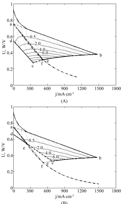
Figure 2. Diagrammatic representation of process and re-sults of determining the cell interior OFO and MCP curves in the cell absolute lifetime ranges of (A) La≥La,f and (B) La ≤La,f in the case of μ≠ 0 and β = 0. See Figure 1 for part

annotations and see Section 2.2.1 for more details.

Figure 3. Diagrammatic representation of process and re-sults of determining the cell interior OFO and MCP curves in the cell absolute lifetime ranges of (A) La≥La,f and (B) La ≤La,f in the case of μ≠ 0 and β≠ 0. See Figure 1 for part

annotations and see Section 2.2.1 for more details.

with the relative lifetime end-curve and the absolute life- time end-curve. See the following discussions for the detailed implications of the related terms.

The values of cell constants for illustration in Figures 1-3 are given in Table 1. The values are also used for the figures in other sections.

2.2.2. Load Interior OPO and MCP Curves

According to Formula (1) or (11), in the interior of the working zone, the ECR of the PEM fuel cell power gen- eration is the one-variable differentiable function of cur- rent density under the condition of any given load power density. Thus the condition for the load interior MCP point is:

0 d

j

j l j

 

_

Table 1. Cell constant values for illustrations.

α(Ω·cm2_{) β(Ω·cm}2_·h−1_{) λ(V) Μ(V·h}−1_{) L}

a(h)

Figure 1 0.257 2.083 × 10−5 _{0.751 0 32,784}

Figure 2(A) 0.257 0 0.751 8.333 × 10−6 _42,998

Figure 2(B) 0.257 0 0.751 8.333 × 10−6 _15,000

Figure 3(A) 0.257 2.083 × 10−5 _{0.751 8.333 × 10}−6 ₂₅₀₀₀

Figure 3(B) 0.257 2.083 × 10−5 _{0.751 8.333 × 10}−6 _11,000

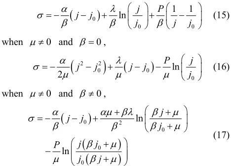
tion. The load interior OFO equation has three expres- sions in total depending on different degradation charac- teristics, as shown in Formulae (15)-(17).

0

  and  0, when





0 0

1 1

j P

j j j

 

  

   

        

   

0

 (15)

when   and  0,









0 ln

P j

j

j

 

  

 

    _{ }

 

0

0 0

2 j j j

   (16)

when   and  0,













0 2

0

0

ln

j j

j j P

j j

0

ln j

j

    



   

 

  

 

 

  _{ }



 

  

 _ _



 

0  

(17)

Substituting P = Uj into Formulae (15)-(17) turns the load interior OFO equation into their second form given as:

when   and  0,





0 0

1

j U j

j j

 

  

   

  _{ } _  _

   

0

   (18*)

when   and  0,









0

ln

Uj j

j

 

  

 

    _{ }

 

0

0 0

2 j j j j

   (19*)

when   and  0,













0 2

0

0

ln

j j

j j Uj

j j

0

ln j

j

    



   

 

  

 

 

    _{ }



 

  

 _ _



 

(20*)

In Formulae (18*)-(20*),

2 ₄

2

Uj

  



 

W U

0

j  (21*)

In U-j plane, Formulae (18*)-(20*) present themselves as a curve at any cost factor. Termed as the load interior OFO curve, the curve is composed of the OFO points

under the conditions of the same economic factor but different load power densities in the interior of the working zone. Thus with a series of cost factor values, Formulae (18*)-(21*) separately turn into a contour plot, a group of thin solid curve as shown in Figures 1-3.

Because the load interior OFO equation is valid only in the interior of the working zone, the cost factor at the intersection point of the relative and absolute lifetime end-curves may be the upper limit to the application of the equations. As seen from Figures 1-3, the contour curve gradually moves down as cost factor increases. Moreover, the equation does not always apply to the whole load power density range even if cost factor is smaller than the upper limit, which can be clearly seen from Figures 1-3.

Substituting P = Uj and Formula (14) into Formula (11) gives Formula (22). It reveals the completely equal relationship between economic voltage and operating vol- tage regardless of cell degradation characteristic. Accord- ingly, Formulae (18*)-(20*) can be directly changed into those for the load interior MCP point only by substituting

W for U in them, and then they are called the load inte- rior MCP equation and present themselves as a curve in

W-j plane called the load interior MCP curve. It is obvi- ous that the load interior OFO and MCP curves are of point- to-point correspondence and superposed on each other.

(22) The existence of the relationship like Formula (22) may mean one set of formulae may be enough to repre-sent the evolution of the cell interior MCP and OFO points. The complete superposition of the load interior OFO and MCP curves may naturally lead to that of the cell interior OFO and MCP curves. Since W and U can be inter- changed, it is certain the two cell interior curves share a set of formulae. This is why the symbol * is given after the formula sequence numbers. The same practice will be followed in Sections 2.2.3 and 2.2.4 where the cell OFO curve is not given discussion any more. And when the formulae marked with the symbol * are men-tioned in the final treatment, their implications should be understood in context.

2.2.3. Cell Unconditional Interior MCP Curve

Formulae (23*)-(25*) can be derived. j0 in Formulae (24*) and (25*) is shown in Formula (21*).

when  0 and  0 0

j

,

(23*) when 0 and 0,

0 ln 

  1

j j

j W

 

 

 

0

(24*)

when   and  0,









0

ln j j

j

j j

 

 

 

  

 

 _ 

  1

j W

 



 _  _

2

W j

(25*)

Formulae (23*)-(25*) all are called the cell precise un- conditional interior MCP equation, and this is to distin- guish it from the cell approximate unconditional interior MCP equation derived latter on. Unconditional means the infinity of the relative and absolute lifetimes, and

precise should be understood in a relative sense as the equation is always based on the ideal cell model. In W-j

plane, each of Formulae (23*)-(25*) present itself as a curve, the bold dashdotted curve as separately shown in

Figures 1-3. As the assembly of the cell interior MCP points under different economic factors, the curve is called the cell precise unconditional interior MCP curve.

The Equations (24*) and (25*) look as if they were simple, but they are very complicated actually. Then Formulae (26*) and (27*) can be used as substitutes for them.

 

   (26*)

8

9 5

4

j

 

W 



 _   _ 

 

0

(27*)

Formulae (26*) and (27*) are called the cell approxi- mate unconditional interior MCP equation. They actually present themselves as a straight line, af, as shown in

Figures 2 and 3. The cell approximate unconditional in- terior MCP curve has the same starting point but differ- ent intersection point with the relative lifetime end-curve from the cell precise unconditional interior MCP curve. In fact, the cell approximate unconditional interior MCP curve is decided jointly by the cell precise unconditional interior MCP curve, the cell approximate unconditional relative lifetime boundary MCP curve and the relative lifetime end-curve. See Section 2.4 for details on this aspect.

Due to simplicity and small error, the following dis- cussions about the latter two degradation characteristics ( and 0, 0 and  0

0

) will be devel- oped around the cell approximate unconditional interior MCP curve. And the term the cell unconditional interior MCP curve used in the following discussions for the two

degradation characteristics exactly refers to the cell ap- proximate unconditional interior MCP curve, unless other- wise stated. For the first degradation characteristic,

  and  0, there are no terms the cell approxi- mate unconditional interior MCP curve and equation. Thus the term the cell precise unconditional interior MCP curve is now changed into the cell unconditional interior MCP curve that will be used in the following discussions.

2.2.4. Cell Conditional Interior MCP Curve

Considering the finity of the relative and absolute life- times, the cell unconditional interior MCP curve turns into the cell conditional interior MCP curve. Here there are three cases in total corresponding to the three degra- dation characteristics.

1) Case of 0 and 0

0 

As shown in Figure 1, in the case of   and 0, the cell unconditional interior MCP curve is al- ways located outside of the working zone however long the absolute lifetime is. It is the very zero current density line, and this means the load interior MCP keeps mo- notonously decreasing with the increase of load power density under any cost factor. So nothing but the absolute lifetime end-curve, the straight line segment ac, can act as the cell conditional interior MCP curve under this first degradation characteristic.

2) Case of 0 and  0 0

In the case of  and  0, both the cell un- conditional interior MCP curve is a straight line only determined by the initial SSP constants α and λ inde- pendent of the degradation constant μ. As shown in Fig-ures 2(A) and 2(B), the straight line passes through the working zone and intersects with the relative lifetime end-curve at point f for a long cell absolute lifetime, or intersects with the absolute lifetime end-curve at point f and suppositionally does with the relative lifetime end-curve at point f for a short cell absolute lifetime. Here, the criterion to judge the absolute lifetime is short or long is the length of the absolute lifetime at point f. Such a length is critical and thus called the critical abso- lute lifetime, denoted by La,f, as shown in Formula (28).

As seen from Formula (28), for the second degradation characteristic, the critical absolute lifetime of the cell is determined only by μ and λ and has no relation with other cell constants.

,

3

a f

L   (28) 

in the interior of the working zone, and this conceptual renewal applies henceforward. As shown in Figure 2(A), when a a f, , the cell unconditional interior MCP

curve is the straight line segment af, and the cell condi- tional interior MCP curve is one part of the relative life- time end-curve, the straight line segment fc. As shown in

Figure 2(B), when a a f, , the cell unconditional in-

terior MCP curve is the straight line segment

L L

L L

af, and the cell conditional interior MCP curve is one part of the absolute lifetime end-curve, the straight line segment f c.

3) Case of  0 and  0

L L

The structure of the cell interior MCP curve in this third case is similar to that in the second case. However, there are two major differences. One is that the critical absolute lifetime is determined jointly by four cell con- stants, α, λ, β and μ, as shown in Formula (29). The other is that, when a a f, , the cell conditional interior

MCP curve (fc) presents itself as a curve segment as it is one part of the relative lifetime end-curve

, ₄

a f

L  9 8 3

 

 

 _   _

  (29)

2.2.5. Applicable Cost Factor Range of Cell Interior MCP Curves

The applicable cost factor ranges of the load interior MCP equation is just those of the cell interior MCP curve. However, the range needs to be further decomposed be- cause of the various configurations of the cell interior MCP curves. And there are three cases in total corre- sponding to the three degradation characteristics.

1) Case of  0 and  0

In this first case, determined by the finity of the cell absolute lifetime, nothing but the cell conditional interior MCP curve is the very cell interior MCP curve. And the applicable cost factor range is   c (xdenotes the

cost factor magnitude at operating point x). c can be

gained by substituting the coordinates of operating point

c into Formula (18*). The coordinates of operating point

c are:





2 c 2

a

W L

c

j  

  

 (30*)

2) Case of  0 and  0

L L

In this second case, the applicable cost factor range depends on the magnitude of the cell absolute lifetime.

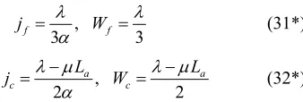
If _{a a f,} , the cell interior MCP curve, the bold dash curve shown in Figure 2(A), is composed of the straight curve segments af and fc. Their applicable cost factor ranges are   _f and _f   _c, respec- tively. _f and _c can be gained by substituting the coordinates of the coordinates of operating points f and c, respectively, into Formula (19*). They are given in For- mulae (31*) and (32*).

,

3 3

f f

j  W 

 (31*)

 

,

2 2

a a

c c

L L

j   W  



 

 

L L

(32*)

If _a _{a f,} , the cell interior MCP curve, the bold dash curve shown in Figure 2(B), is composed of the straight curve segments af and f c. Their applicable cost factor ranges are   f and f  c, re-

spectively. _f and c can be gained by substituting

the coordinates of the coordinates of operating points

f and c, respectively, into Formula (19*). The coordi-nates of operating point c is shown in Formula (32*), and those of operating p nt oi f are given in Formula (33*).

, 2

a

f f a

L

j  W  L



   (33*)

In the case of this second degradation characteristic, the cell precise unconditional interior MCP curve (the curve ae) is a curve determined only by the initial SSP constants α and λ independent of the degradation con- stant μ, as shown in Figures 2(A) and (B). It intersects the relative lifetime end-curve at point e whose coordi- nates are given in Formula (34*).

0.341 _{, 0.341}

e e

j  W 



 

0

(34*)

As known from Formulae (31*) and (34*), operating points f and e are highly close to each other. As seen from Figures 2(A) and 2(B), it may be rational and con- venient to substitute the cell precise unconditional inte- rior MCP curve with the cell approximate unconditional interior MCP curve, and a major error may not be pro- duced. It can be proved that the cell precise uncondi- tional interior M-ECR curve does not get tangental to the absolute lifetime end-curve in the interior of the working zone however long the absolute lifetime is. This is also an important reason to treat the cell unconditional inte- rior curve as a straight line.

3) Case of  and  0

In terms of the applicable cost factor range, this third case is similar to the second case. And the dividing cost factor magnitudes can be gained by substituting the co- ordinates of the related operating points as given in For- mulae (35*)-(37*) into Formula (20).

8

9 3 ,

4

8

9 3

2 8

f

f

j

W

 

 

  

 

 

 _   _

 

  (35*)

  _   _

 





2 2

a a

c c

a

L L

j W

L

   

 

 

 





4 _,

8

9 1 4

8

1 9

4

a f

a a

5

f a

W L

a

L j

L

L

L  

 



 _{ }

 

  



 

 

  

 

 

 

 





  

 



 

 

 

e f

(37*)

As seen from Figures 3(A) and (B), in this third case, the intersection point e of the cell precise unconditional interior MCP curve with the relative lifetime end-curve may likewise be close to the point f. So it may be rational and of little error to approximately treat the cell uncondi-tional interior MCP curve as a straight line. We fail to find the analytical expressions of the coordinates of the point e, but it can be validated that the cell precise un-conditional interior MCP curve does not get tangental to the absolute lifetime end-curve in the interior of the working zone however long the absolute lifetime is.

2.3. Cell Relative Lifetime Boundary MCP Curve

2.3.1. Diagrammatic Representation

Figures 4-6 display the process and results of determin- ing the cell relative lifetime boundary MCP curve (the bold dash curve) for the three degradation characteristics. In these figures, the thin solid curves are a series of load relative lifetime boundary cost performance (CP) curves of equal cost factor with 106 _C·cm−2 _{as the unit of charge}

density. The bold dashdotted curve is the cell precise unconditional interior MCP curve; fh is the cell approxi- mate unconditional interior MCP curve; cg is the cell conditional relative lifetime boundary MCP curve; af is the cell unconditional interior MCP curve; the bold dot- ted curve, the thin dotted curve and the thin solid curves all play auxiliary roles. Point g is the intersection point of curve cg and line W = 0, and point f is the intersection point of curve eh, curve fh and line W = 0. See Section 2.2 for the implications of bold solid curves ab, bc, cd,

da and points a, b, c, d, e, f, and . See the fol- lowing discussions for the detailed implications of the related terms.

2.3.2. Load Relative Lifetime Boundary CP Curve

When cell operating time gets as long as relative lifetime

Lr under load power density P, the operating point arrives

at the relative lifetime boundary end-curve. Here, the economic voltage can be expressed as:

0

d F d

r j

F r _j

L P

j L  l j





r

r L

L P W

j l

 

 

  (38)

Substitute Formula (4) into Formula (38), then the re- lationship between economic voltage and power density

Figure 4. Diagrammatic representation of process and re- sults of determining the cell relative lifetime boundary MCP curve in the case of μ = 0 and β ≠ 0. The bold dash curve stands for the resultant cell relative lifetime boundary MCP curve, and the thin solid curves stand for a series of load relative lifetime boundary CP curves of equal eco- nomic factor. The economic factor values are given with 106 C·cm−2 _{as the unit. See Section 2.3.1 for more details. See} Section 2.2.1 for more details.

Figure 5. Diagrammatic representation of process and re- sults of determining the cell relative lifetime boundary MCP curves in the cell absolute lifetime ranges of (A) La≥

La,f and (B) La≤La,f in the case of μ≠ 0 and β = 0. See

Figure 6. Diagrammatic representation of process and re-sults of determining the cell relative lifetime boundary MCP curves in the cell absolute lifetime ranges of (A) La≥

La,f and (B) La≤La,f in the case of μ≠ 0 and β≠ 0. See

Fig-ure 4 for part annotations and see Section 2.3.1 for more details.

can be derived. Called the load relative lifetime boundary (cost performance) CP equation, the relationship present itself as three analytical expressions as shown in Formu- lae 39 - 41 depending on the three degradation character- istics. j0 and jF in Formulae (39)-(41) are given in

For-mulae (11) and (13), respectively. when 0 and  0,





r

F

r F F

L P W

L j  j j 



 



 

    _{ }

 0  0

1 1

F

j P

j  j j

 

 _  _

 

0 when

(39)

 and  0,









0 0

0

ln 2

r

F

r F F F

L P W

j P

L j j j j j

j

 



  



 

      _{ }

 

0

(40) when  and  0,

According to our recent works, the relative lifetime can be expressed with Formulae (42)-(44) under load power density P for the three degradation characteristics. when 0 and 0,

2

4

r

L P

 

  (42)

 

0

when  and  0, 2

r

P

L  



 

0

(43)

when   and  0,





2 2 2

2

2 2

r

P P P

L     



   



0

(44)

When the relative lifetime end comes under load power density P, the relationship between load power density P and current density jr is given in Formulae (45) -

(47).

when   and 0,

2 r

j

P  (45)

0

when  and  0, 2

r

P j (46) 0

 when  and  0,





2

r

r

j P

j  

 

 



0

(47)

Separately substitute Formulae (42) and (45) into For-mula (39), ForFor-mulae (43) and (46) into ForFor-mula (40) and Formulae (44) and (47) into Formula (41), then the sec- ond form of the load relative lifetime boundary CP equa-tion can be obtained for the three degradaequa-tion character- istics, as shown in Formulae (48)-(50).

when   and 0,

0

0 0

2 2

ln 2

F

F F

j W

j j

j

j j

   

  

 _ 

 

 



 

   _{ }

 

(48)













0 2

0 0

ln ln

r

F F

r F F

r

L P W

j j

j P

L j j j

j j j

 

 

  



      



  

  



    

(41)

 

 _  _

when  0 and 0,





j _{j j}

        0 3 _ln 2 2 F F F j j                (49)

when  0 and 0,



























F F F F F F

j j j W j j j j j

j j j j j j

      0 0 ln F F F j j j                                     _  _ _{ }  _{  }  _          _  _ (50)

Initial current densities j0 in Formulae (48)-(50) are given in Formulae (51)-(53), respectively.

2 ₂ 2 0 F j      

j  (51)

2 ₄ 2 2

2 0 F j      





j  (52)

2 2 0 4 2 2 F F j j        j     

 (53)

Under any cost factor, each of Formulae (48)-(50) pre- sents itself as a curve in W-j plane. It is called the load relative lifetime boundary CP curve as it is composed of the CP points under different load power densities at the relative lifetime boundary. For a series of cost factors, each of Formulae (48)-(50) gives a group of load relative lifetime boundary CP curves with different cost factors, as shown in Figures4-6.

Although the load relative lifetime boundary CP curve moves with cost factor, the load relative lifetime bound- ary final operating (FO) curve keeps unchanged, and it is the very relative lifetime end-curve. The load relative lifetime boundary CP and FO curves are of point-to-point correspondence, but they are not superposed.

3.3.3. Cell Unconditional Relative Boundary MCP Curve

Make dW/djFin Formulae (48)-(50) equal to zero and get

rid of σ by using Formulae (48)-(50), then Formulae (54)-(56) can be obtained. Initial current densities j0 in Formulae (55) and (56) are given in Formulae (52) and (53), respectively

when  0 and  0 0

F

j  ,

(54) when  0 and  0,

0 3 ln 1 F F j j j W  

       0 (55)

when   and  0,













2 ln 1

F F F F F F j j W j j j j j j                

       (56)

  _{ } _ _ 

 

   

 

Formulae (54)-(56) all are called the cell precise un-conditional relative lifetime boundary MCP equation. This is to distinguish it from the cell approximate uncon-ditional relative lifetime boundary MCP equation derived latter on. Unconditional refers to the infinitely long ab-solute lifetime. In W-j plane, each of Formulae (54)-(56) presents itself as a curve, the bold dashdotted curve as separately shown in Figures 6-10. The curve is called cell precise unconditional relative lifetime boundary MCP curve, as it is the assembly of the cell precise un- conditional relative lifetime boundary MCP points under different cost factors. The intersection point of the cell precise unconditional relative lifetime boundary MCP curve and the corresponding load relative lifetime boun- dary CP curve is just the cell precise unconditional rela- tive lifetime boundary MCP point under a given cost factor.

Formulae (55) and (56) look as if they were simple, but they are very complicated actually. The cell precise unconditional relative lifetime boundary MCP curve corre- sponding to Formula (55) or (56) is only in a small current density range as shown in Figure 4 or 5, so, it may be substituted with a constant current density line that passes through its intersection point with the line W = 0. The corresponding mathematical expressions are given as Formula (57) or (58).

3 F

j   (57) 

8

9 3

4

F

j  

 

 

 _   _

  (58)

Figure 7. Diagrammatic representation of process and re-sults of determining the cell absolute lifetime boundary MCP curve in the case of μ= 0 and β≠ 0. The bold dash curve stands for the resultant cell absolute lifetime bound-ary MCP curve, and the thin solid curves stand for a series of load absolute lifetime boundary CP curves of equal eco-nomic factor at regular intervals of ecoeco-nomic factor. The economic factor values are given with 106 _C·cm−2 _{as the unit.} See Section 2.4.1 for more details.

Figure 8. Diagrammatic representation of process and re- sults of determining the cell absolute lifetime boundary MCP curves in the cell absolute lifetime ranges of (A) La≥

La,f and (B) La≤La,f in the case of μ≠ 0 and β= 0. See

Fig-ure 7 for part annotations and see Section 2.4.1 for more details.

Figure 9. Diagrammatic representation of process and re- sults of determining the cell absolute lifetime boundary MCP curves in the cell absolute lifetime ranges of (A) La≥

La,f and (B) La≤La,f in the case of μ≠ 0 and β≠ 0. See

Fig-ure 7 for part annotations and see Section 2.4.1 for more details.

curve. The cell precise and approximate unconditional relative life- time boundary MCP curves have the same starting point and different intersection points with the relative lifetime end-curve in both cases.

In the case of  0 and  0

0

, the cell precise un- conditional relative lifetime boundary MCP curve, the cell precise unconditional interior MCP curve and the relative lifetime end-curve intersect at point e. So a straight line can be defined with the intersection point of the cell precise unconditional interior MCP curve and the line j = 0 as one point and with the intersection point of the cell approximate unconditional relative lifetime boundary MCP curve and the relative lifetime end-curve as the other. Such a straight line, af, is just the cell ap- proximate unconditional interior MCP curve, as shown in

Figure 10. The composition of the cell MCP and OFO curves for (A) long and (B) short cell absolute lifetimes in the case of μ = 0 and β≠ 0. See text for more details.

Due to simplicity and small error, the following dis- cussions about the two degradation characteristics,

0

  and

Under any degradation characteristic, although the cell unconditional relative lifetime boundary MCP point moves with cost factor and thus forms the cell uncondi-tional relative lifetime boundary MCP curve, the cell unconditional OFO point keeps unmoved. That is to say, the whole cell unconditional relative lifetime boundary MCP curve belongs to one cell OFO point in the relative lifetime end-curve. Here, there is no concept like the cell unconditional relative boundary OFO curve.

3.3.4. Cell Conditional Relative Lifetime Boundary MCP Curve

0

  ,  0 and  0, will be devel- oped around the cell approximate unconditional relative lifetime boundary MCP curve. And the term the cell un- conditional relative lifetime boundary MCP curve used in the following discussions for the two degradation characteristics exactly refers to the cell approximate un- conditional relative lifetime boundary MCP curve, unless otherwise stated. Correspondingly, the term the cell con- ditional relative lifetime boundary MCP curve refers to the cell approximate conditional relative lifetime bound- ary MCP curve. For the first degradation characteristic,

0

  and  0

0

, there are no term the cell approxi- mate unconditional relative lifetime boundary MCP curve or equation. Thus the term the cell precise uncon- ditional relative lifetime boundary MCP curve is now changed into the cell unconditional relative lifetime boundary MCP curve that will be usedin the following discussions.

Considering the finity of the cell absolute lifetime, the cell unconditional relative lifetime boundary MCP curve turns into the cell conditional relative lifetime boundary MCP curve.

In the case of   and  0





, as shown in Figure 4, the line j = 0 is just the cell unconditional relative life- time boundary MCP curve. This means the monotonous decrease of the load relative lifetime boundary CP as the increase of current density under any cost factor. So, nothing but the constant current density line (cg) passing through the intersection point of the absolute and lifetime end-curves (c) acts as the cell relative lifetime boundary MCP curve, because of the finity of the cell absolute life- time. It is the cell conditional relative lifetime boundary MCP curve whose mathematical expression is given as Formula (59).

2

F

a

j

L



(59)  

 

In the other two cases, as shown in Figures 5 and 6, the constant current density line fh corresponding to point f is just the cell unconditional relative lifetime boundary MCP curve. This means the monotonous in- crease of the load relative lifetime boundary CP as the increase of current density in the range of jF jf and

the monotonous decrease in the range of F f under

any cost factor, if the cell absolute lifetime is infinitely long.

j  j

The finity of the absolute lifetime restricts the load relative lifetime boundary CP curve within the current density range of F c. As shown in Figures 5(A) and

6(A), when a a f, , the cell unconditional relative

lifetime boundary MCP curve fh lies in the current den- sity range of

j  j L L

F c, so it is surely the cell relative life-

time boundary MCP curve. As shown in Figures 5(B)

and 6(B), when a a f, j  j

L L , the cell unconditional relative lifetime boundary MCP curve fh does not lie in the range of F c, so it can’t act as the cell relative lifetime

boundary MCP curve. Here, the constant density line cg

passing through point c is the veritable cell relative life- time boundary MCP curve, and it is the cell conditional relative lifetime boundary MCP curve. Formulae (60) and

0

(61) give the mathematical expressions of the line cf, re- spectively, in the case of   and

arrives at the absolute lifetime end-curve. Here, the eco- nomic voltage can be expressed as:

0

  and the

case of  0 and 0.

2

a

L



F

j  

  





(60)

2

a a

L L

   

 

ic

ic

c g

ic ic

F 

j

c ic

(61)

Similar to the cell unconditional relative lifetime boundary MCP curve, the whole cell conditional relative lifetime boundary MCP curve belongs to one cell OFO point in the relative lifetime end-curve for any degrada- tion characteristic. And likewise, there is no concept like the cell conditional relative boundary OFO curve

3.3.5. Applicable Cost Factor Range of Cell Relative Lifetime Boundary MCP Curve

As seen from Figures 4-6, the cell relative lifetime boun- dary MCP curve applies to the whole cost factor range from zero to infinity for any cell degradation characteris- tic.

3.4. Cell Absolute Lifetime Boundary MCP Curve

3.4.1. Diagrammatic Representation

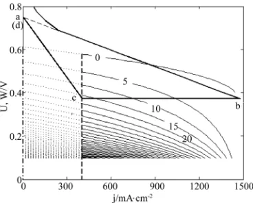
Figures 7-9 display the process and results of determin- ing the cell absolute lifetime boundary MCP curve (the bold dash curve) for the three cell degradation character-istics. In these figures, the thin solid curves are a series of load absolute lifetime boundary CP curves of equal cost factor with 106 _C·cm−2 _{as the unit of charge density. The}

bold dashdotted curve is the cell first precise abso-lute lifetime boundary MCP curve. is the cell first approximate absolute lifetime boundary MCP curve.

is the cell second absolute lifetime boundary MCP curve. The bold dotted curve, the thin dotted curve and the thin dash curve are displayed for assistant roles. Point

i is the intersection point of curves , and line j =

0, and points and are separately the intersection points of and with line cg. See Section 2.2 or 2.3 for the implications of other points and curves and see the following discussions for the implications of new terms.

c ic 

3.4.2. Load Absolute Lifetime Boundary CP Curve

When cell operating time gets as long as absolute life- time La under load power density P, the operating point

0

0 d d

a F

a a

L j

F a _j

L P L P

W

j l j L l j

 

 



_

_

0

Substituting Formula 4 into Formula 62 gives the rela- tionship between economic voltage and load power den- sity, and this is called the load absolute lifetime boundary CP equation. There are three expressions of the load ab- solute lifetime boundary CP equation in total depending on cell degradation characteristic, as shown in Formulae 63 - 65.

when   and 0,





0 0

1 1

ln

a F

a F F

F

L P W

j P

L j j j

j j j

 



  



   

    _{ } _  _

   

0

(63) when   and  0,









0 0

0

ln 2

a

F

a F F F

L P W

j P

L j j j j j

j

 



  



 

      _{ }

 

0

(64) when   and  0,

In Formulae (62)-(65), j0 and jF are given as Formulae

(8) and (9), respectively.

According to Formulae (3) and (6), when the cell op- erates until the absolute lifetime end-point under load power density P, the relationship between the load power density and current density are expressed as Formulae (66)-(68):

when  0 and 0,





a F F

P    L j j

0

(66)

when   and  0,





2

F a F

P j    L j

0

(67)

when   and  0,









a F a F

P    L j    L j (68)

Separately substituting Formula (66) into (63), For-mula (67) into ForFor-mula (64) and ForFor-mula (68) into (65) give the second form of the load absolute lifetime boun- dary CP equation, as shown in Formulae (69)-(71).













0 2

0 0

ln ln

a

F F

a F F

r

L P W

j j

j P

L j j j

j j j

 

 

  



      

 (65)

  

  



     _   _ 

when  0 and  0,













a F a F

a F F

L j L j

W

L j j j

                          _{ }

 0 0

1

a F

F L j F

j j

j  j

 



 

 

(69)

when  0 and 0,

















0 0

2

a F a F

F a

a F F F

L j L j

W

j L

L j j j j j

                     0 ln F F j j j         (70)

when  0 and 0,













_



_



0 0

F

r

j j

j

0 2 ln ln

a F a a F

F a a F

F

a F F

L j L L j

W

j L L j

j

L j j j

j j                                             _{ }           _  _ (71)

In Formulae (69)-(71), initial current densities are se- parately given as:





2 ₄ 2 ₄

a F F

L j j

0 ₂

j     



  

  





(72)

2 2 2

0

4 4

2

F a F

j    L j





j   



  

 (73)





j     



   

    L ja F ₍₇₄₎

In W-j plane, Formulae (69) and (70) all present them- selves as a curve under any cost factor. The curve is composed of the load CP points under different load power densities at the absolute lifetime boundary and thus called the load absolute lifetime boundary CP curve. For a series of cost factors, each of Formulae (69)-(71) gives a group of load absolute lifetime boundary CP curves with different cost factors

In order to observe the evolution of the load absolute lifetime boundary CP as economic factor, a series of load absolute lifetime boundary CP curves over the complete current density range are given in Figures 7-9, respec- tively, according to Formulae (69)-(71). However, owing to the restriction of the cell absolute lifetime, the load absolute lifetime boundary CP equation is valid only in the current density range of _{F c}, while invalid in the

range of j j



F c. In Figures 7-9, the valid and invalid

parts of the load absolute lifetime boundary CP curves are display as the thin solid curves and the dotted curves, respectively.

j 

0

j

Although the load absolute lifetime boundary CP curve moves with cost factor, the load absolute lifetime boundary FO curve keeps unchanged, and it is the very absolute lifetime end-curve. The load absolute lifetime boundary CP and FO curves are of point-to-point corre- spondence, but they are not superposed.

3.4.3. Cell Absolute Lifetime Boundary MCP Curve

Make dW/djF in Formulae(69)-(71) equal to zero and get

rid of σ by using Formulae (69)-(71), then two solutions can be obtained for each cell degradation characteristic. The first solution is given as Formulae (75)-(77) and the second is given as Formulae (59)-(61)

when  and 0,

0

1 1 a

F

L

j j W



(75)

 

0

when  and  0,

0

ln jF La

j W         0 (76)

when  and  0,









0

ln F a

F

j j L

j j W

            _    ic c g (77)

In Formulae (75)-(77), initial current densities j0 are given separately as Formulae (72)-(74).

In W-j plane, Formulae (75)-(77) all present themselves as a curve, the bold dashdotted curve in Figures 7-9, called the cell first precise absolute lifetime boundary MCP curve for the corresponding cell degradation char- acteristic. This is to distinguish it from the cell first ap- proximate absolute lifetime boundary MCP curve that will occur latter on. Formulae (59)-(61) all present them- selves as a straight line of equal current density, the straight line 

W W 

c

W

in Figures 7-9, called the cell second absolute lifetime boundary MCP curve. As seen from

Figures 7-9, the cell precise absolute lifetime boundary MCP curve is actually a devious curve composed of the cell first precise absolute lifetime boundary MCP curve in the economic voltage range of c and the cell