warwick.ac.uk/lib-publications
Manuscript version: Author’s Accepted Manuscript
The version presented in WRAP is the author’s accepted manuscript and may differ from the
published version or Version of Record.
Persistent WRAP URL:
http://wrap.warwick.ac.uk/72190
How to cite:
Please refer to published version for the most recent bibliographic citation information.
If a published version is known of, the repository item page linked to above, will contain
details on accessing it.
Copyright and reuse:
The Warwick Research Archive Portal (WRAP) makes this work by researchers of the
University of Warwick available open access under the following conditions.
Copyright © and all moral rights to the version of the paper presented here belong to the
individual author(s) and/or other copyright owners. To the extent reasonable and
practicable the material made available in WRAP has been checked for eligibility before
being made available.
Copies of full items can be used for personal research or study, educational, or not-for-profit
purposes without prior permission or charge. Provided that the authors, title and full
bibliographic details are credited, a hyperlink and/or URL is given for the original metadata
page and the content is not changed in any way.
Publisher’s statement:
Please refer to the repository item page, publisher’s statement section, for further
information.
Preprocessing Reference Sensor Pattern Noise via
Spectrum Equalization
Xufeng Lin and Chang-Tsun Li,
Senior Member, IEEE
Abstract—Although sensor pattern noise (SPN) has been
proven to be an effective means to uniquely identify digital cameras, some non-unique artifacts, shared amongst cameras undergo the same or similar in-camera processing procedures, often give rise to false identifications. Therefore, it is desirable and necessary to suppress these unwanted artifacts so as to improve the accuracy and reliability. In this work, we propose a novel preprocessing approach for attenuating the influence of the non-unique artifacts on the reference SPN to reduce the false identi-fication rate. Specifically, we equalize the magnitude spectrum of the reference SPN through detecting and suppressing the peaks according to the local characteristics, aiming at removing the interfering periodic artifacts. Combined with 6 SPN extraction or enhancement methods, our proposed Spectrum Equalization Algorithm (SEA) is evaluated on the Dresden image database as well as our own database, and compared with the state-of-the-art preprocessing schemes. Experimental results indicate that the proposed procedure outperforms, or at least performs comparably to, the existing methods in terms of the overall ROC curve and kappa statistic computed from a confusion matrix, and tends to be more resistant to JPEG compression for medium and small image blocks.
Index Terms—Multimedia forensics, source camera identifica-tion (SCI), sensor pattern noise, spectrum equalizaidentifica-tion, PRNU
I. INTRODUCTION
A
DVANCES in digital imaging technologies have led to the development of low-cost and high-quality digital imaging devices, such as camcorders, digital cameras, scanners and built-in cameras of smartphones. The ever-increasing con-venience of image acquisition has facilitated the distribution and sharing of digital images, and bred the pervasiveness of powerful image editing tools, allowing even unskilled persons to easily manipulate digital images for malicious or criminal ends. Under the circumstance where digital images serve as the critical evidences, forensic technologies that help verify the origin and authenticity of digital images become essential to a forensic investigator. One challenging problem of multimedia forensics is source camera identification (SCI), the task of which is to reliably match a particular digital image with its source device.Despite the methods based on metadata, or watermarking embedded in the image, are effective to prove the source of an image, unfortunately they are infeasible under many cir-cumstances. For example, the metadata might not be available, and legacy images might not be watermarked at the time when
X. Lin and C.-T. Li are with the Department of Computer Science, Universi-ty of Warwick, Coventry, CV4 7AL, U.K. (e-mail: [email protected]; [email protected]).
they were created. In view of the limitation, researchers have switched their attentions to the methods that search for the intrinsic characteristics of digital cameras left in the image. Generally speaking, any inherent traces left in the image by the processing components, either hardware or software, of the image acquisition pipeline, such as defective pixels [1, 2], color filter array (CFA) interpolation artifacts [3, 4], JPEG compression artifacts [5, 6], lens aberration [7, 8] or the combination of several image intrinsic characteristics [9, 10], can be utilized to link the images to the source camera. Apart from the above-mentioned techniques, the methods that attract the most attention may be those based on SPN [11–17], which mainly consists of the photo-response non-uniformity (PRNU) noise [11] arising primarily from the manufacturing imperfections and the inhomogeneity of silicon wafers. The uniqueness to individual camera and stability against envi-ronmental conditions make SPN a feasible fingerprint for identifying and linking source cameras.
The typical process of using SPN for SCI is as follows: reference SPN R is first constructed by averaging the noise residual Wi extracted from the ith image of the N images
taken by the same camera:
R= 1
N
N X
i=1
Wi. (1)
The similarity between the reference SPN R and the query noise residue W is measured by the normalized correlation coefficient (NCC)ρ:
ρ(R,W) = PM
k=1
PN
l=1(W(k, l)−W)(R(k, l)−R)
kW −Wk · kR−Rk , (2)
wherek · k is the L2 norm, R andW are of the same size
M ×N and the mean value is denoted with a bar. Suppose the reference SPN of camerac isRc, the task of SCI is then
achieved by identifying camera c∗ with the maximal NCC value that is greater than a predefined threshold τρ as the
source device of the query image, i.e.,
c∗= argmax
c∈C
ρ(Rc,W), ρ(Rc∗,W)> τρ, (3)
where C is the set of candidate cameras. However, the correlation-based detection of SPN heavily relies upon the quality of the extracted SPN, which can be severely contami-nated by image content, color interpolation, JPEG compression and other non-unique artifacts. In order to guarantee the accuracy and reliability of identification, the size of SPN has to be very large, for example,512×512pixels or above. But
Copyright (c) 2015 IEEE. Personal use of this material is permitted.
the large size of SPN limits its applicability in some scenarios. One example is image or video forgery localization [12, 18– 23], where there exists a trade-off between localization and accuracy. Another scenario is digital camcorder identification [24], where the spatial resolution of video frames is usually much smaller than that of typical still images. One more example is camera fingerprints (SPNs) clustering [25–27]. The complexity of clustering is usually very high and the high dimension of SPNs will further bring difficulties to computation and storage. The clustering algorithm is expected to use the lower length of SPNs but still guarantee good performance. Therefore, exploring the ways of improving the quality of SPNs extracted from small-sized image blocks becomes of great significance for the above-mentioned SPN-based applications.
Over the past few years, many efforts have been devoted to improving the performance of SPN-based source cameras identification. Proposed approaches in the literature can be grouped into two categories as follows. Approaches of the first category aim to better estimate or select the reference SPN. For example, Chenet al.[12] proposed a maximum likelihood estimation (MLE) of the reference SPN from several residual images. They also proposed two preprocessing operations, zero-mean (ZM) and Wiener filter (WF), to further remove the artifacts introduced by camera processing operations. In [28], Hu et al. argued that the large or principal components of the reference SPN are more robust against random noise, so instead of using the full-size SPN, only a small number of the largest components are involved in the calculation of correlation. Some works focus on the enhancement of the SPN. For example, Li [15] assumed that the stronger a signal component of SPN is, the more likely it is associated with strong scene details. Consequently, 6 enhancing models were proposed to attenuate the interference from scene details. In the later work [23], Liet al.proposed a color-decoupled PRNU (CD-PRNU) extraction method to prevent the interpolation noise from propagating into the physical components. They extracted the PRNU noise patterns from each color channel and then assembled them to get the more reliable CD-PRNU. Another enhancement method is proposed by Kang et al. in [16], where a camera reference phase SPN is introduced to remove the periodic noise and other non-white noise con-taminations in the reference SPN. As we are actually dealing with the noise residuals, the choice of denoising filters has a great impact on the performance [28, 29]. With this in mind, Chierchia et al.[18] proposed to use an innovative denoising filter, block-matching and 3D filtering (BM3D) [30], to replace the Michak denoising filter [31]. BM3D works by grouping 2D image patches with similar structures into 3D arrays and collectively filtering the grouped image blocks. The sparseness of the representation due to the similarity between the grouped blocks makes it capable of better separating the true signal and noise. Another SPN extractor, edge adaptive SPN predictor based on context adaptive interpolation (PCAI), was proposed in [17, 32] to suppress the effect of scenes and edges.
The second category of approaches attempts to improve the source device identification rate through the use of more sophisticated detection statistics or similarity measurements.
Goljan [33] proposed the peak-to-correlation energy (PCE) measure to attenuate the influence of periodic noise contami-nations
PCE(R,W) = C
2
RW(0,0)
1
M N−|A|
P
(k,l)∈A/ C
2
RW(k, l)
, (4)
where CRW is the 2D circular cross correlation between
R and W, A is a small area around (0,0), and |A| is the cardinality of the area. Later in [16], Kang et al.proposed to use the correlation over circular cross-correlation norm (CCN) to further decrease the false-positive rate:
CCN(R,W) =q CRW(0,0)
1
M N−|A|
P
(k,l)∈A/ C
2
RW(k, l)
, (5)
where all the symbols have the same meanings as in Equation (4). Actually CCN shares the same essence as the signed PCE (SPCE) [14, 34]
SPCE(R,W) = sign(CRW(0,0))C
2
RW(0,0)
1
M N−|A|
P
(k,l)∈A/ C
2
RW(k, l)
, (6)
where sign(·)is the sign function, and all the other symbols have the same meanings as in Equation (4). Surely, the above-mentioned approaches can be combined for additional performance gains. For instance, one can apply ZM and WF operations on the reference SPN extracted with BM3D or PCAI algorithm, and enhance the query noise residual with the help of Li’s models [15], and finally choose SPCE or CCN as the similarity measurement to identify the source camera.
work on SCI in the absence of counter-forensics can increase our confidence in decision-making, but in turn can more easily arouse our suspicion in the presence of counter-forensics, e.g. the SPNs have been maliciously removed and cause strange detection results. Most importantly, the techniques developed for the scenarios without the presence of counter-forensics usually can facilitate to expose the counter-forensics, and they are probably still effective when dealing with the recovered information from counter-counter-forensics.
In this paper, we propose a new preprocessing scheme, namely Spectrum Equalization Algorithm (SEA), for the reference SPN to enhance the performance of SCI. If the reference SPN is modeled as white Gaussian noise (WGN), the theoretical analysis of WGN points out that the reference SPN should have a flat magnitude spectrum. Peaks appearing in the spectrum are probably originated from the periodic artifacts and unlikely to be associated with the true SPN. Therefore, by detection and suppressing the peaks in the spectrum, we can obtain more clean (noise-like) signals. We will start by studying the limitations of existing preprocessing schemes, and then propose our SEA in detail to overcome the limitations.
The paper is organized as follows. In Section II, we revisit the previous works through a case study and point out the limitations of existing preprocessing approaches. The details of the proposed preprocessing scheme, SEA, are presented in Section III. Comprehensive experimental results and analysis for both the general and special cases are given in Section IV. Finally, Section V concludes the work.
II. RELATEDWORK ONSPN PREPROCESSING
As can be found in Section I, most literature [12, 16, 28] focuses on the processing of the reference SPN, only Li’s enhancers [15] are applied on the query noise residual. The reason is that, the noise residual extracted from a single image can be severely contaminated by interfering artifacts arisen from scene details, CFA interpolation, on-sensor signal transfer [40], JPEG compression and other image processing operations. Therefore, it is extremely difficult to distinguish the true SPN from the estimated SPN. While in the reference SPN, the random artifacts, such as the shot noise, read-out noise and quantization noise, have been averaged out. Moreover, if the camera is available, we can take high-quality images, such as blue sky or flatfield images, to better estimate the reference SPN. As a result, we can easily incorporate our prior knowledge of SPN to refine the estimated signal. In [12], for example, Chen et al. proposed the ZM procedure to remove the artifacts introduced by CFA interpolation, row-wise and column-row-wise operations of sensors or processing circuits, as well as theWFprocedure to suppress the visually identifiable patterns in theZM processed signal. Specifically, row and column averages are deducted from every pixel in the corresponding row and column of the reference SPNRto form the zero-meaned reference SPNRzm. TheWFprocedure
is carried out by transforming Rzm into the discrete Fourier
transform (DFT) domain,Dzm, and applying the Wiener filter
on each frequency index(u, v)
Dwf(u, v) =Dzm(u, v)
σ2 0
ˆ
σ2(u, v) +σ2 0
, (7)
whereσ2
0represents the overall variance ofRzm, andσˆ2(u, v)
is the maximum a posterior estimation of the local variance
ˆ
σ2(u, v) = min w∈{3,5,7,9}
max0, 1
w2
X
(k,l)∈Nw
D2zm(k, l)−σ20
,
(8) whereNw is a w×w local neighborhood centered at(u, v).
The final reference SPN Rwf is obtained by applying the
inverse discrete Fourier transform (IDFT) onDwf.
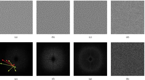
Fig. 1 shows the results of different operations on the
256×256reference SPN, which is estimated from 50 blue sky images captured by Canon PowerShot A400 using BM3D [30]. It is worth mentioning that although we used the noise residues extracted using BM3D [30], similar results can be observed for the SPNs extracted using other extraction methods [11, 12, 32]. As a reference, random white noise and the corresponding spectrum are also illustrated in Fig. 1d and 1h, respectively. The white noise is drawn from the normal distribution with zero mean and the same variance as the original SPN shown in Fig. 1a. SPNs in the spatial domain are shown in the first row, and the corresponding DFT magnitude spectra are shown in the second row (for the purpose of visualization, the zero-frequency component has been shifted to the center of the spectrum). Unless otherwise specified in this paper, we use the term “spectrum” to refer to the DFT magnitude spectrum hereinafter. As can be seen from the first column of Fig. 1, although there exists no obvious periodic pattern in the spatial domain, the peaks resulted from the periodic artifacts can be easily identified in the DFT domain. As we know that the peaks associated with one signal with periodT will appear in the locations (UTu,VTv), where U andV are the dimensions of the spectrum, and u, v ∈ {0,1, ..., T −1}. Thus, what is striking in Fig. 1e is that most of the peaks are resulted from the artifacts with period 8 (as indicated by the green arrows), but some of them are brought about by the artifacts with period 16 (as indicated by the red arrows). Due to the symmetry of the spectrum, only the peaks in one quadrant are illustrated in Fig. 1e. But as shown in Fig. 1f, after applying the
ZMoperation, the horizontal and vertical DC components are completely removed as hinted by the two “dark” intersecting lines passing through the center of the spectrum. Though the magnitudes of other frequency components remain quan-titatively unchanged, the remaining peaks become visually more distinct as the peaks with dominating values have been removed. ZM removes all the DC components in the spectrum, so any artifacts lying in the two central “dark” lines will be also removed. However, when comparing with the spectrum in Fig. 1h, we found that ZM seems overly aggressive in modifying the DC components. If theWFoperation is further applied to theZMfiltered SPN in the DFT domain, we can get the resultant image and the corresponding spectrum as shown in Fig. 1c and 1g, respectively. According to Equation (7), a magnitude spectrum coefficient,Dzm(u, v), with a larger local
(a) (b) (c) (d)
[image:5.612.58.559.51.327.2](e) (f) (g) (h)
Fig. 1: Filtering for the reference SPN of Canon PowerShot A400. (a) Original SPN, (b) ZM filtered SPN, (c) ZM + WF
filtered SPN, (d) white noise, (e) spectrum of the original reference SPN, (f) spectrum of the ZMfiltered reference SPN, (g) spectrum of the ZM + WFfiltered reference SPN, (h) spectrum of white noise. Note that the intensity of the figures has been linearly scaled into[0,1]for visualization purpose.
therefore is suppressed more significantly. As a consequence, the spectrum in Fig. 1g looks “flatter” than that in Fig. 1f. So with the help of ZM and WF, three improvements have been made: 1) any artifacts appearing in DC components are completely removed, 2) the spectrum is more noise-like (flat) and 3) the peaks arisen from periodic artifacts are significantly suppressed. Despite the peaks in the low-frequency region have been suppressed effectively, those in the high-frequency region are less affected, which can be clearly seen from the “white” points in Fig. 1g. Therefore, in view of the effects of ZM and WF, it seems that ZM is overly aggressive in modifying the DC components and WF appears to be too conservative in suppressing the peaks in the high-frequency band. These leave room for improvement.
III. SPECTRUMEQUALIZATIONALGORITHM(SEA)
As mentioned at the start of Section II, the “purity” of the reference SPN makes it more suitable to be modified by incorporating prior knowledge of SPN, such as the fact that the true SPN signal is unlikely to be periodic and should have a flat spectrum. But the key problem is how to incorporate the prior knowledge appropriately and modify the reference SPN accordingly. When comparing the spectra of theZMand
WF filtered SPN with that of white noise, we can see that the horizontal and vertical DC components are completely removed and the peaks in the high-frequency band are still visible. Besides, we are actually not confident in modifying the low-frequency components, which probably have been
severely contaminated by scene details. So without enough information to ensure the global “flatness”, can we just ensure the local “flatness” of the spectrum by simply removing the salient peaks? Identifying the periodic artifacts responsible for the prominent peaks in the spectrum can help us better understand the problem and find an appropriate solution. We summarize the periodic artifacts as follows.
• CFA interpolation artifacts. A typical CFA
interpo-lation is accomplished by estimating the missing com-ponents from spatially adjacent pixels according to the component-location information indicated by a specific CFA pattern. As CFA patterns form a periodic structure, measurable offset gains will result in periodic biases in the interpolated image [12]. The periodic biases manifest themselves as peaks in the DFT spectrum, and the lo-cations of the peaks depend on the configuration of the CFA pattern.
• JPEG blocky artifacts. In JPEG compression,
non-overlapping 8 × 8 pixel blocks are coded with DCT independently. So aggressive JPEG compression causes blocky artifacts, which manifest themselves in the DFT spectrum as peaks in the positions (U8u,V8v), where U and V are the sizes of the spectrum, and u, v ∈ {0,1, ...,7}.
• Diagonal artifacts. As reported in [41], unexpected
spectrum as peaks in the positions corresponding to the row and column period introduced by the diagonal artifacts.
Given that the noise-like SPN should have a flat spectrum without salient peaks, the rationale, which forms the basis of the proposed SEA for preprocessing the reference SPN, is that
the peaks present in the DFT spectrum are unlikely to be associated with the true SPN, and the unnatural traces usually
appear in the form of periodic patterns, such as the 2×2 or
4×4 CFA patterns,8×8JPEG blockiness and so on, which
correspond to the peaks in fixed positions of spectrum. By suppressing these peaks, SPN of better quality can be obtained.
SEA consists of peak detection and peak suppression, as detailed in Procedure 1 and Procedure 2, respectively. The peaks in the spectrum of the reference SPN are detected by comparing the ratio of the spectrum to the local mean with a threshold, as shown in Step 12 and 13 of Procedure 1. When calculating the local mean within a neighborhood wcentered at(u, v)in Step 8 and 9 of Procedure 1, the tilde sign “∼” over P1 and P2 is the logical negation operator, which excludes
the spectral components indicated by the logical0s inP1and
P2 from the calculation of the local mean M.L(·) in Step
12 and 13 labels any nonzero entry of input to logical ‘1’ and zero to logical ‘0’, so the peaks in D will be disclosed by the logical 1s stored in P1 and P2. The above steps are
repeated 3 times to make the peak detection more accurate. Finally in Step 17, ‘&’ and ‘|’ are the logical AND and OR operator, respectively, so the potential spurious peaks not at the indices(U
16u,
V
16v), u= 0,1, . . . ,15, andv= 0,1, . . . ,15are
screened out. Having identified the peak locations, the peaks are suppressed by simply replacing them with the local mean intensities in the spectrum, as shown in Step 4 of Procedure 2. There are several remarks need to be made for SEA:
• We use two thresholds τ1 and τ2, with τ1 < τ2, for
peak detection in Step 12 and 13 of Procedure 1. The underlying motivation for this particular consideration is to detect peaks more liberally by using a smaller threshold τ1in Step 12 to avoid missing peaks in positions indicated
byBin Step 16 of Procedure 1, but more conservatively by using a larger thresholdτ2in Step 13 in other positions
to avoid distorting the true SPN. Because spurious peaks are more likely to be detected with a smaller thresholdτ1,
suppressing these spurious peaks will probably distort the true SPN. But with a larger threshold τ2, the prominent
peaks can be detected without worrying about being excessively modified.
• We only consider the artifacts with a period of up to 16 pixels. Albeit the fact that the artifacts sometimes appear with different periods, such as the3×3or6×6CFA pat-tern, and they may also contain components with period larger than 16. The justification is twofold: 1) the2×2
and4×4 are the most common CFA patterns; 2) peaks caused by the artifacts with other periods may overlap in the peak locations hinted inB. For example, half of the peaks caused by the 32×32periodic signal will appear in the peak locations of B. As a consequence, peaks in positions indicated by B account for the dominant
components caused by the majority of periodic artifacts, which is consistent with our observation in Fig. 1 and the following experiments in Section IV-E. Even if the prominent peaks are missed out byB, they will still be caught out by P2.
• Although some similarity measurements, such as PCE, CCN or SPCE, also aim at suppressing the periodic noise contamination, there are two fundamental differ-ences between our SEA and the aforementioned similarity measurements:
1) The calculation of the similarity measure involves the reference SPN and the query noise residual. Howev-er, the query noise residual is likely to be severely contaminated by other interfering artifacts. As a con-sequence, even for the query noise residual extracted from a high-quality image, the periodic patterns are very inconspicuous, making the peaks discovered by circular cross correlation not so remarkable as those found in the spectrum of the reference SPN.
2) The similarity measurements require extra computation for every SPN pair, which will largely increase the computational complexity. However, with the proposed SEA, we only need to apply it on the reference SPN once for all, which will save a considerable amount of time for large databases.
Procedure 1Spectrum Peak Detection
Input:
R: original reference SPN of U×V pixels; w: size of a local neighborhood;
τ1,τ2: two thresholds for peak detection,τ1< τ2;
Output:
P:U×V binary map of detected peak locations;
1: Calculate the magnitude spectrum D=DFT(R);
2: Initialize twoU×V binary mapsP1=P2=0; 3: Initialize twoU×V mean matricesM1=M2=0; 4: count= 0;
5: repeat
6: foru= 1 toU do
7: forv= 1 toV do
8: M1(u, v) =
P
(k,l)∈Nw|D(k,l)|P˜1(k,l) P
(k,l)∈NwP˜1(k,l) ;
9: M2(u, v) =
P
(k,l)∈Nw|D(k,l)|P˜2(k,l) P
(k,l)∈NwP˜2(k,l) ;
10: end for
11: end for
12: P1=L |M1D| ≥τ1
;
13: P2=L |
D|
M2 ≥τ2
;
14: count=count+ 1;
15: untilcount >2
16: Create aU×V binary matrix B, with 1s only at indices
(16Uu,16Vv), u, v= 0,1, . . . ,15;
17: Screen out spurious peaks P =P1&B|P2;
Procedure 2 Spectrum Peak Suppression
Input:
R: original reference SPN ofU×V pixels; P:U ×V detected peak locations;
w: size of a local neighborhood;
Output:
RSEA:U×V spectrum equalized reference SPN;
1: D=DFT(R);
2: foru= 1 toU do
3: forv= 1 toV do
4: L(u, v) =
P
(k,l)∈Nw|D(k,l)|P˜(k,l) P
(k,l)∈NwP˜(k,l)
;
5: end for
6: end for
7: RSEA=IDFT(LD|D|);
8: returnRSEA;
IV. EXPERIMENTS
A. Experimental Setup
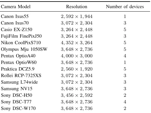
We first evaluated the performance of the proposed pre-processing scheme on the Dresden Image Database [42]. The basic information of the used cameras can be found in Table I. 49 cameras, covering 15 models and10 brands, that have contributed 50 flatfield images were chosen. The 50 flatfield images were used to estimate the reference SPN for each camera, and another 150 natural images captured by the same camera served as query images. As mentioned in [41], unexpected artifacts were observed in the estimated reference SPN of Nikon CoolPixS710, FujiFilm FinePixJ50 and Casio EX-Z150, so we will take special care for the 13 cameras of these 3 models after analyzing the remaining 36 cameras as the general cases.
Apart from the effectiveness, the robustness of the proposed scheme against JPEG compression was also investigated on our own uncompressed image database, as detailed in Table II. 600 natural images taken in BMP format by 6 cameras were used in this experiment. The images contain a wide variety of natural indoor and outdoor scenes taken during holidays, around campus and cities, in offices and sports center, etc. Among the 100 images captured by each camera, 50 were randomly chosen to estimate the reference SPN, and the other 50 were used as query images. For each BMP image, compressed images were produced by libjpeg [43] with quality factor of100%,90%,80%,70%,60%and50%. Therefore,6
groups JPEG images, i.e.,3,600in total, with different quality factors were generated.
[image:7.612.314.561.81.266.2]We aim to compare the performances of different prepro-cessing schemes, but with different SPN extraction techniques continue to appear, it would be interesting to see how well the preprocessing schemes work in conjunction with existing SPN extractors. What is more, comparing the performance of different algorithms on real-world databases provides insight into the advantages and disadvantages of each algorithm, and offers a valuable reference for practical applications. Bearing this in mind, we incorporated 6 SPN extraction or enhance algorithms in the experiments. For the sake of convenience, we refer to the technique in [11] as “Basic”, [12] as “MLE”, [15] as “Enhancer”, [30] as “BM3D”, [16] as “Phase”, and [32]
TABLE I:49 cameras involved in the creation of the images in the Dresden database
Camera Model Resolution Number of devices
Canon Ixus55 2,592×1,944 1
Canon Ixus70 3,072×2,304 3
Casio EX-Z150 3,264×2,448 5
FujiFilm FinePixJ50 3,264×2,448 3
Nikon CoolPixS710 4,352×3,264 5
Olympus Mju 1050SW 3,648×2,736 5
Pentax OptioA40 4,000×3,000 4
Pentax OptioW60 3,648×2,736 1
Praktica DCZ5.9 2,560×1,920 5
Rollei RCP-7325XS 3,072×2,304 3
Samsung L74wide 3,072×2,304 3
Samsung NV15 3,648×2,736 3
Sony DSC-H50 3,456×2,592 2
Sony DSC-T77 3,648×2,736 4
[image:7.612.315.561.309.396.2]Sony DSC-W170 3,648×2,736 2
TABLE II: 6cameras involved in the creation of the images in our own database
Camera Model Resolution Number of images
Canon 450D 4,272×2,848 100
Canon Ixus870 1,600×1,200 100
Nikon D90 4,288×2,848 100
Nikon E3200 2,048×1,536 100 Olympus C3100Z 2,048×1,536 100 Panasonic DMC-LX2 3,168×2,376 100
as “PCAI8”. Although “Enhancer” only enhances the query noise residual and has nothing to do with the noise extraction, hereinafter we refer to all these 6 algorithms as SPN extractors for convenience. For the preprocessing schemes, we refer to zero-mean operation as ZM, the Wiener filter in the DFT domain as WF, the combination of ZM and WF operations as ZM+WF, and the proposed spectrum equalization algorithm as SEA.
B. Parameters Setting
For Basic [11], MLE [12] and Phase [16], we used the source codes published in [14, 34]. For Li’s Enhancers [15], we adopted Model 3 withα= 6because it shows better results than his other models. For BM3D [30], we downloaded the source codes from [44] and simply used the default parameters. To facilitate fair comparison, we set the noise varianceσ2
0= 4
for all the algorithms that use Mihcak filter [31], as well as BM3D and PCAI8.
For the SEA, we do not have the prior information about how strong the periodic artifacts are and how the energy is distributed over the spectrum, so we empirically set the neighborhood size w to 17 and 15 for Procedure 1 and 2, respectively. The thresholds τ1 and τ2 in Procedure 1 are
forgery localization, the experiments were performed on image blocks with different sizes cropped from the center of the full-resolution images due to the vignetting effects [45]. When needed in the rest of this paper, we will use the terms “large”, “medium” and “small” to refer to the sizes of 1024×1024,
256×256 and64×64pixels, respectively. It is worth noting that all preprocessing schemes will only be applied on the reference SPN due to the reason mentioned at the beginning of Section II. In the following experiments, NCC, as defined in Equation (2), will be used as the similarity measurement between the reference SPN and the query noise residual, but the results of SPCE, as defined in Equation (6), will also be presented when necessary.
C. Evaluation Statistics
To demonstrate the performance of the proposed preprocess-ing scheme, we adopted two evaluation statistics, namely the overall receiver operating characteristic (ROC) curve [16, 32] and the kappa statistic [46] computed from a confusion matrix. To obtain the overall ROC curve, for a given detection threshold, the true positives and false positives are recorded for each camera, then these numbers are summed up and used to calculate the True Positive Rate (TPR) and False Positive Rate (FPR). Specifically, as the numbers of images captured by each camera are exactly the same, we can simply calculate the TPR and FPR for a threshold as follows:
TPR= PC
i=1Ti
T
FPR= PC
i=1Fi
(C−1)T,
(9)
where C is the number of cameras, T is the total number of query images, Ti and Fi are the true positives and false positives of camera i, respectively. By varying the detection threshold from the minimum to the maximum value as cal-culated using Equation (2), we can obtain the overall ROC curve.
To obtain the confusion matrix M, we calculated the similarity between the noise residue of one query image and the reference SPN of each camera, then this image was deemed to be taken by the camera corresponding to the maximal similarity. The value of each elementM(i, j)in the confusion matrix indicates the number of images taken by camera i that have been linked to camera j as the source device. In other words, the values along the main diagonal indicate the numbers of correct identifications. Each confusion matrix can be reduced to a single value metric, kappa statistic K [46]:
K= o−e
T −e, (10)
whereois the number of observed correct identifications, i.e., the trace of confusion matrix, T is the total number of query images, andeis the number of expected correct identifications:
e= C X
c=1
PC
i=1M(c, i)
PC
j=1M(j, c)
T , (11)
whereC is the number of cameras. Kappa statistic measures the disagreement between the observed results and random
guess, therefore the larger the value of K, the better the performance, with 1 indicating the perfect performance.
The reason why both the overall ROC curve and the kappa statistic are used is that we want to properly evaluate the per-formances of two different SPN-based real-world applications, SCI and forgery detection, which are the same in essence while differing in minor points. Normally, in the task of forgery detection, the similarity measurement, between the reference SPN and the noise residue extracted from the image block in question, is directly compared with a threshold suggested by some criterion, such as the Neyman-Pearson criterion, to determine whether the image block has been tampered with or not. This process is equivalent to the generation of one point in the ROC curve, therefore it is more appropriate to evaluate the performance of forgery detection using the overall ROC curve. While in the context of SCI, the query image is believed to be taken by the camera with the maximal similarity which is greater than a predefined threshold at the same time. It is more like the process of creating a confusion matrix. So the kappa statistic computed from a confusion matrix is a preferable evaluation statistic for SCI.
D. General Cases
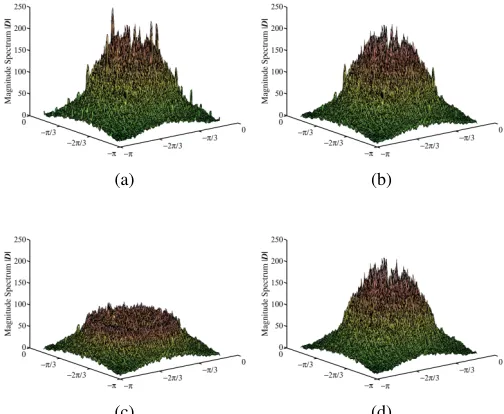
Before delving into the details, let us first look at a straight-forward comparison of the effects of different preprocessing on the spectrum of the reference SPN. Fig. 2a-2c are the corresponding spectra of the reference SPNs shown in Fig. 1a-1c, while Fig. 2d shows the spectrum of the SEA filtered SPN. To reduce the dynamic range of magnitudes and make the peaks more conspicuous, a5×5averaging filter is convolved with the spectrum beforehand. As can be clearly seen in Fig. 2d, when compared with the spectrum processed by the ZM and ZM+WF, the “spiky” interferences have been nicely smoothed out by SEA while the rest of the spectrum still remains untouched. In this manner, the true SPN has been preserved as much as possible.
(a) (b)
(c) (d)
[image:8.612.314.566.505.712.2]0 100 200 300 400 500
Probability Density
−0.05 0 0.05 ρ 0
100 200 300 400 500
Probability Density
−0.05 0 0.05 ρ 0
100 200 300 400 500
Probability Density
−0.05 0 0.05 ρ 0
100 200 300 400 500
−0.05 0 0.05 ρ
Probability Density
0 20 40 60 80 100 120
Probability Density
−0.05 0 0.05 ρ 0
20 40 60 80 100 120
Probability Density
−0.05 0 0.05 ρ 0
20 40 60 80 100 120
Probability Density
−0.05 0 0.05 ρ 0
20 40 60 80 100 120
−0.05 0 0.05 ρ
Probability Density
0 5 10 15 20 25 30
Probability Density
−0.05 0 0.05 ρ 0
5 10 15 20 25 30
Probability Density
−0.05 0 0.05 ρ 0
5 10 15 20 25 30
Probability Density
−0.05 0 0.05 ρ 0
5 10 15 20 25 30
−0.05 0 0.05 ρ
[image:9.612.56.559.50.326.2]Probability Density
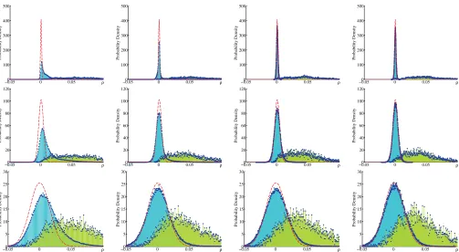
Fig. 3: Estimated inter-class and intra-class PDFs of ρcalculated from SPNs extracted from3different sizes of image blocks using BM3D. From top to bottom, the rows show the distributions for image blocks sized1024×1024,256×256and64×64
pixels, respectively. From left to right, the distributions are resulting from the original reference SPN and the ones preprocessed by ZM, ZM+WF and SEA, respectively.
The advantages of SEA can also be observed in Fig. 3, where we show the estimated inter-class (in light blue color) and intra-class (in light green color) probability density functions (PDFs) of the correlation valueρfor the 36 cameras in the Dresden database. The values outside the range of
[−0.05,0.1]are cut off to make the figures look more compact. As shown in the first column, due to the long right-hand tail of the inter-class distribution, there are a considerable amount of overlaps between the inter-class and intra-class distributions if no preprocessing is applied. After ZM and WF are applied sequentially, the long tail on the right-hand side of the inter-class distribution is curtailed and the inter-inter-class variances significantly decrease from 2.46×10⁻⁴, 3.49×10⁻⁴ and
6.04×10⁻⁴ to 1.44×10⁻⁶, 2.65×10⁻⁵ and 3.55×10⁻⁴
for large, medium and small image blocks, respectively. As a result, the overlaps between the inter-class and intra-class correlation distribution are reduced substantially. Compared with the inter-class distribution brought about by ZM+WF, the resulting inter-class distribution of SEA looks even “thinner”, with a smaller variance 1.89×10⁻⁵ and 2.95×10⁻⁴ for
medium and small image blocks, respectively. The smaller variance of inter-class distribution makes the two distributions more separable from each other, and therefore boosts the performance. For the large size, 1024 ×1024 pixels, the variance of inter-class distribution for SEA is 1.47×10⁻⁶, which is slightly larger than that of ZM+WF, 1.44×10⁻⁶. But the intra-class mean for SEA,0.05, is slightly larger than the0.045for ZM+WF. So considering these two aspects, SEA
and ZM+WF are comparable to each other in the case of large image blocks, which will also be quantitatively reflected in Fig. 4 and 5. In addition, we can see that the inter-class distribution resulting from SEA fits quite well to the theoretical distribution, which is a normal distribution with 0 mean and
1/d variance (in red dashed lines), where d is the length of SPNs.
0.00010 0.001 0.01 0.1 FPR 0.2 0.4 0.6 0.8 TPR
0.00010 0.001 0.01 0.1 FPR 0.2
0.4 0.6 0.8 TPR
0.00010 0.001 0.01 0.1 FPR 0.2
0.4 0.6 0.8 TPR
0.00010 0.001 0.01 0.1 FPR 0.2
0.4 0.6 0.8 TPR
0.00010 0.001 0.01 0.1 FPR 0.2
0.4 0.6 0.8 TPR
0.00010 0.001 0.01 0.1 FPR 0.2
0.4 0.6 0.8 TPR
0.00010.001 0.01 0.1 FPR 0 0.2 0.4 0.6 0.8 TPR
0.00010.001 0.01 0.1 FPR 0 0.2 0.4 0.6 0.8 TPR
0.0001 0.001 0.01 0.1 FPR 0 0.2 0.4 0.6 0.8 TPR
0.0001 0.001 0.01 0.1 FPR 0 0.2 0.4 0.6 0.8 TPR
0.00010.001 0.01 0.1 FPR 0 0.2 0.4 0.6 0.8 TPR
0.00010.001 0.01 0.1 FPR 0 0.2 0.4 0.6 0.8 TPR
0.00010 0.001 0.01 0.1 FPR 0.2 0.4 0.6 0.8 TPR Basic Basic+ZM Basic+ZM+WF Basic+SEA
0.00010 0.001 0.01 0.1 FPR 0.2 0.4 0.6 0.8 TPR MLE MLE+ZM MLE+ZM+WF MLE+SEA
0.00010 0.001 0.01 0.1 FPR 0.2 0.4 0.6 0.8 TPR Enhancer Enhancer+ZM Enhancer+ZM+WF Enhancer+SEA
0.00010 0.001 0.01 0.1 FPR 0.2 0.4 0.6 0.8 TPR Phase Phase+ZM Phase+ZM+WF Phase+SEA
0.00010 0.001 0.01 0.1 FPR 0.2 0.4 0.6 0.8 TPR BM3D BM3D+ZM BM3D+ZM+WF BM3D+SEA
0.00010 0.001 0.01 0.1 FPR
[image:10.612.55.561.52.243.2]0.2 0.4 0.6 0.8 TPR PCAI8 PCAI8+ZM PCAI8+ZM+WF PCAI8+SEA
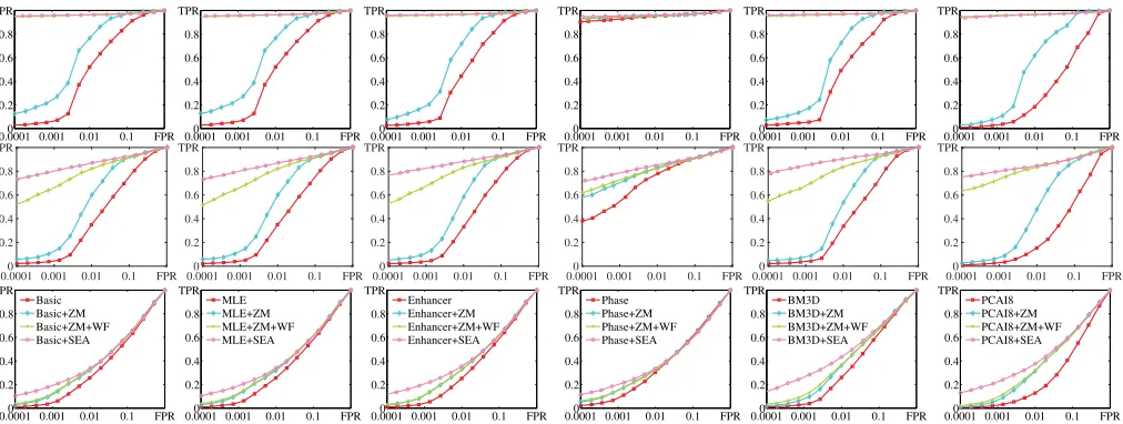
Fig. 4: Overall ROC curves of the combinations of different SPN extractors and preprocessing schemes (different columns) on different image block sizes (different rows). From top to bottom, the rows show the ROC curves for large, medium and small image blocks, respectively. Please refer to the last row for the legend text, which is the same for the figures in the same column.
Original ZM ZM+WF SEA
0 0.2 0.4 0.6 0.8 1
Basic MLE Enhancer
Phase BM3D PCAI8
(a)
Original ZM ZM+WF SEA
0 0.2 0.4 0.6 0.8 1
Basic MLE Enhancer
Phase BM3D PCAI8
(b)
Original ZM ZM+WF SEA
0 0.2 0.4 0.6 0.8 1
Basic MLE Enhancer
Phase BM3D PCAI8
[image:10.612.82.527.308.434.2](c)
Fig. 5: TPRs at the FPR of 1×10⁻³ for image blocks sized (a)1024×1024(b) 256×256and (c) 64×64pixels.
superiority of SEA over ZM+WF is not so apparent as that in the case of large image size, because they are both around the corner of perfect performance. When it comes to image blocks sized 64×64 pixels, all the investigated SPN-based methods seem to run into a bottleneck, but preprocessing the reference SPN can still push the performance upward.
Fig. 5 depicts the TPRs at a FPR as small as 1×10⁻³.
The dark red dotted line shows the average of each group cor-responding to one preprocessing scheme. Averagely speaking, preprocessing can substantially increase the TPR at a low FPR. Similar with the observation in Fig. 3, SEA is equally matched with ZM+WF for large image size, but has higher TPRs than ZM+WF for medium and small sizes. With regard to different SPN extractors, Phase is the most special one among all the 6 extractors. It is stable against various preprocessing, resulting in its outstanding position when preprocessing is not applied. The underlying reason is that Phase only retains the phase component but ignores the magnitude components of each noise residual that is used to estimate the reference SPN. In this way, the periodic artifacts have been suppressed considerably but not completely removed. So preprocessing can further, although slightly, improve the performance of
Phase, as can be seen from the green bins in Fig. 5. The performance of Basic, MLE and Enhancer are equivalent in many respects, but Enhancer more or less outplays the other two when combined with SEA. Interestingly, BM3D and PCAI8 perform worse than the other SPN extractors when no or little preprocessing is applied, but they apparently sweep the board with the help of ZM+WF or SEA. By using the non-local information to get the better noise estimation, it is not surprising that BM3D performs consistently best among all 6 extractors in case of being combined with SEA. It is also worth mentioning that PCAI8 performs even worse than Phase when combined with ZM or ZM+WF. This is probably due to the insufficiency of images to create trustworthy reference SPN [32].
TABLE III: Kappa statistics for1024×1024image blocks
Preprocessing
Original ZM ZM+WF SEA
Basic 0.9236 0.9644 0.9691 0.9684
MLE 0.9236 0.9646 0.9695 0.9682
Enhancer 0.9059 0.9623 0.9722 0.9701
Phase 0.9650 0.9632 0.9610 0.9629
BM3D 0.9192 0.9651 0.9718 0.9714
[image:11.612.314.561.71.171.2]PCAI8 0.7366 0.9545 0.9701 0.9691
TABLE IV: Kappa statistics for256×256 image blocks
Preprocessing
Original ZM ZM+WF SEA
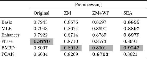
Basic 0.7943 0.8676 0.8697 0.8895
MLE 0.7943 0.8674 0.8697 0.8897
Enhancer 0.7922 0.8714 0.8785 0.8979
Phase 0.8770 0.8710 0.8573 0.8691
BM3D 0.8097 0.8912 0.8901 0.9242
PCAI8 0.6634 0.8269 0.8703 0.8621
bold value in a row signifies the best preprocessing scheme for the corresponding extraction method of the row. So the optimal combination of extraction method and preprocessing scheme is the entry in both gray background and bold font style. As shown in the 3 tables, most of the bold numbers appear in the last two columns, indicating the effectiveness of ZM+WF and SEA. The most apparent example is PCAI8, of which the kappa statistic increases by approximately 0.2
after preprocessed by ZM+WF or SEA when the image block size is 256×256 pixels. For the case of 64×64 blocks, in spite of the insignificant performance declines, the reference SPNs extracted with the Michak filter seem to be vulnerable to preprocessing. But for the other two extractors, BM3D and PCAI8, the performance gain can still be guaranteed. Special attention should be paid to Table III, where ZM+WF performs slightly better than SEA. The average kappa statistic gap 0.0006, between SEA and ZM+WF, is negligible when compared with the average kappa statistic gain 0.0162 and
0.02in the cases of medium and small image blocks, respec-tively. To understand it more intuitively, we took a close look at the confusion matrix. We found that, for image blocks sized
1024×1024pixels, ZM+WF has only about an average of 3
more correctly classified images than SEA among the 5400
images from36cameras. But the average number of correctly classified images by SEA is around 85 and 105 more than ZM+WF for the medium and small image blocks, respectively. As for different extractors, Basic, MLE and Enhancer perform comparably well in all conditions. This is consistent with our observations in Fig. 4 and 5. As indicated by the gray backgrounds in the 3 tables, BM3D shows a clear superiority over other extractors. Moreover, with the help of SEA, BM3D exhibits the superior (or at least equivalent) performance over other combinations for all block sizes. Therefore, the joint use of BM3D and SEA is preferable for both forgery detection and SCI in practice.
JPEG is probably the most common image format used in
TABLE V: Kappa statistics for64×64image blocks
Preprocessing
Original ZM ZM+WF SEA
Basic 0.4116 0.4067 0.3962 0.4070
MLE 0.4122 0.4072 0.3952 0.4086
Enhancer 0.4061 0.4030 0.3907 0.4044
Phase 0.4055 0.3735 0.3724 0.3859
BM3D 0.4838 0.4865 0.4625 0.5046
PCAI8 0.3918 0.4166 0.4010 0.4276
digital cameras, so we compared the robustness of ZM+WF and SEA against JPEG compression. The experiments were carried out for different image sizes and different SPN extrac-tors. Sometimes the source devices are available to capture high-quality images for reference SPN estimation. So under this scenario, we can use the reference SPN estimated from images with a high quality factor 100% for each of the 6 cameras in Table II, and calculate the similarity between the high-quality reference SPN and the query noise residual extracted from images with different quality factors. But the more plausible scenario is that only the images rather than the source devices are available. So we simulated this scenario by estimating the reference SPN using the images with the same JPEG quality as the query images. The ratios of the kappa statistics of SEA to that of ZM+WF for these two scenarios are shown in the first and second column of Fig. 6, respectively. The dark red dotted lines show the average of each group corresponding to one quality factor. A ratio greater than 1 indicates that SEA outplays ZM+WF. We adjusted the y-axis limits to accommodate bins with various heights. As indicated by the dotted lines, the generally higher average ratios in the second column benefit from SEA’s potent capability of removing the more evident JPEG artifacts in the reference SPN estimated from more aggressively compressed images. For the medium (the second row) and the small (the third row) image size, most of the average kappa statistics are higher than 1, indicating SEA’s superiority over ZM+WF. The growing preponderance of the ratios as the images undergo more aggressive JPEG compression, especially in the second column, indicates that SEA tends to be more robust against JPEG compression for medium and small image blocks. But surprisingly, ZM+WF performs better than SEA in the case of large image blocks. We carefully investigated the spectra of the 6 cameras and found that unlike the peaks spreading out over the spectrum, as shown in Fig. 1e, all the prominent peaks appear in the borders of the spectrum and the locations indicated by the two “dark” lines in Fig. 1f, which can be completely removed by ZM. But for large images, the components overly modified by ZM are not so considerable as for small images. Therefore, it introduces bias in favor of ZM+WF for large image size. Another cause comes from the fact that by using larger image blocks, it is more likely to have a more enriched and spread-out spectrum, and therefore make some of the peaks fade away into the background. It is also the reason why SEA limits the further improvement for large blocks in Fig. 4 and Table III.
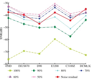
[image:11.612.50.297.205.304.2](S-NR) of noise residue (extracted from the uncompressed bmp images) and JPEG quantization noises to the uncompressed images for each of the 6 cameras. As shown in Fig. 7, when the JPEG quality factor drops to70%, the SNR of quantization noise is even higher than that of noise residual for 4 of the 6 cameras. It indicates that the impact of JPEG compression on the quality of SPN and thus the identification performance can be significant. For example, with256×256blocks, when the quality factor of the query images decreases from100%to
70%, the average kappa statistic over 6 extractors dramatically declines from 0.9433to0.6533for SEA, and from 0.9460to
0.6360 for ZM+WF in the first scenario, and even lower in the second scenario, with an average kappa statistic 0.5767
for SEA and 0.5487 for ZM+WF. But the effects of JPEG compression appear to be much less severe for 1024×1024
sized blocks. Even for the 50% quality factor and the second scenario, the average kappa statistics are still considerable, with0.7680for SEA and 0.7800for ZM+WF. So with large enough block size, even if the images undergo heavy JPEG compression, accurate SCI is still possible.
E. Special Cases
As mentioned in [41], some unexpected artifacts, which may stem from the dependencies between sensor noise and special camera settings or some advanced in-camera post-processing, were observed in the images taken by Nikon CoolPixS710, FujiFilm FinePixJ50 and Casio EX-150. More specifically, a diagonal pattern can be clearly seen in the reference SPN of Nikon CoolPixS710 in the spatial domain and manifests itself as peaks in the DFT domain (see Fig. 8a and 8b). As the diagonal structures are only observed in images taken by CoolPixS710, it is probably due to the spe-cial in-camera post-processing in CoolPixS710. For FujiFilm FinePixJ50, the identification results have a relationship with the difference between the exposure times when capturing the images used for estimating the reference and the image used for extracting the query noise residual. It is possibly that some exposure-time-dependent post-processing procedure is employed in FinePixJ50, for instance to suppress the noise [41]. The experimental results also confirm that SPNs of FinePixJ50 at exposure times ≥ 1/60s exhibit pixel shifts in horizontal direction. The worst case among the three models is Casio EX-150, the identification performance of which is very poor for images taken at different focal length settings. The image distortions become clear by showing the p-maps [47] of images acquired by EX-150. The origin of the artifacts are still unknown to us, but it reminds us to pay particular attention to these 3 models. Thus, separate experiments have been conducted for the 13 cameras of these 3 special models. We only conducted the experiments on blocks of 256 ×256 pixels, since similar properties and trends were observed for other sizes. The kappa statistics based on both NCC and SPCE are listed in Table VI-VIII for a more comprehensive comparison. Comparing the kappa statistics of different preprocessing schemes in Table VI-VII, we found that SEA can improve the performance for Nikon CoolPixS710 and FujiFilm FinePixJ50. When taking a closer
100% 90% 80% 70% 60% 50% 0.8
0.9 1 1.1
Basic MLE Enhancer Phase BM3D PCAI8
100% 90% 80% 70% 60% 50% 0.8
0.9 1 1.1
Basic MLE Enhancer Phase BM3D PCAI8
100% 90% 80% 70% 60% 50% 0.8
0.9 1 1.1 1.2
Basic MLE Enhancer Phase BM3D PCAI8
100% 90% 80% 70% 60% 50% 0.8
0.9 1 1.1 1.2
Basic MLE Enhancer
Phase BM3D PCAI8
100% 90% 80% 70% 60% 50% 0.8
1 1.2 1.4 1.6 1.8 2 2.2 2.4 2.6
Basic MLE Enhancer Phase BM3D PCAI8
100% 90% 80% 70% 60% 50% 0.8
1 1.2 1.4 1.6 1.8 2 2.2 2.4 2.6
[image:12.612.313.562.66.402.2]Basic MLE Enhancer Phase BM3D PCAI8
Fig. 6: Ratios of the kappa statistic of SEA to that of ZM+WF for the cases of estimating the reference SPN from JPEG images with a quality factor 100 (first column) and JPEG images with the same quality factor as the query images (second column). Bins are grouped according to the quality factor of the query images, and each of the 6 bins in the same group shows the ratio for one of the 6 SPN extractors. From top to bottom, the rows show the results for image blocks sized
1024×1024,256×256and64×64pixels.
450D IXUS870 D90 E3200 C3100Z DCMLX2 −80
−70 −60 −50 −40 −30
SNR(dB)
100% 90% 80% 70%
60% 50% Noise residual
[image:12.612.358.511.568.700.2]look at Table VI for Nikon CoolPixS710, the performances of all preprocessing methods are comparable in terms of NCC and SPCE. But compared with ZM+WF, the advantage of SEA becomes obvious in Table VII for FujiFilm FinePixJ50. For instance, the kappa statistic of Enhancer increases from
0.7633to0.8100in terms of NCC, and from0.7700to0.8033
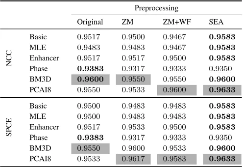
in terms of SPCE. However, for Casio EX-150, in spite of the slight performance gain brought about by preprocessing, correct and reliable identifications are still impossible for the images captured by this model. Another important observation is that the performances of ZM+WF+SPCE and SEA+NCC are comparable for Nikon CoolPixS710 and Casio EX-150, as shown in Table VI and VIII, but SEA+NCC is significantly better than ZM+WF+SPCE for FujiFilm FinePixJ50, as shown in Table VII. Due to the reasons we mentioned in Section III, it is easier to detect the prominent peaks in the spectrum of the reference SPN using SEA than SPCE, attributing to the better performance of SEA+NCC for FujiFilm FinePixJ50. Furthermore, we can see from the last column of Table VI-VIII that SPCE can not further improve the performance of the reference SPN filtered by SEA, or only by a limited amount (for PCAI8). This is due to the fact that the periodic artifacts have been mostly and effectively suppressed by SEA.
Further investigations with the spectra of the 3 camera models, as illustrated in Fig. 8, may unveil the causes of the difference in performance. Because ZM only deals with the DC components, the two peaks associated with the diagonal artifacts reported in [41] are not removable by ZM, as shown in Fig. 8b. The good news is that the two peaks can be well suppressed by both WF and SEA. However, as can be seen from Table VI, the effect of the suppression is not so significant as expected because the energy of the peaks only takes up a small proportion of the overall spectrum energy. For FujiFilm FinePixJ50, although WF can effectively suppress the peaks in the areas with a large local variance, it appears to be helpless in suppressing the peaks in the areas with a small local variance. When zooming in on Fig. 8g, one will find that peaks still exist in the high-frequency band. Despite the much smaller magnitude of the peaks, the overall spectrum has also been substantially reduced at the same time, so the suppression is not so effective as it looks like. This can explain why SEA performs better than ZM+WF for FujiFilm FinePixJ50, as shown in Table VII. Although we are still unable to provide convincing explanations for the poor performance of Casio EX-Z150, as shown in the last row of Fig. 8, the ratio of the energy of low-frequency band to that of high-frequency band seems much higher than those of the other two cameras even in the equalized spectrum, suggesting that the true SPN has been seriously contaminated and making reliable identification difficult. This is probably the reason why the best performance for Casi EX-150 can be achieved by Li’s Enhancer [15], which deals with the scene details lying largely in the central area of the spectrum. Actually the performance on these 3 camera models provides a microcosm of the overall performance: SEA and ZM+WF are comparable for the reference SPN with a relatively smooth spectrum, but SEA is better than ZM+WF for the reference SPNs with a spectrum full of peaks, especially in the high-frequency band. Yet, there exist some
[image:13.612.314.562.120.290.2]unexpected artifacts that both ZM+WF and SEA cannot cope with effectively.
TABLE VI: Kappa statistics for Nikon CoolPixS710 on256× 256 image blocks
Preprocessing
Original ZM ZM+WF SEA
NCC
Basic 0.9517 0.9500 0.9467 0.9583
MLE 0.9483 0.9483 0.9467 0.9583
Enhancer 0.9517 0.9517 0.9500 0.9583
Phase 0.9383 0.9317 0.9333 0.9350
BM3D 0.9600 0.9550 0.9550 0.9600
PCAI8 0.9550 0.9533 0.9600 0.9633
SPCE
Basic 0.9500 0.9483 0.9483 0.9583
MLE 0.9500 0.9483 0.9483 0.9583
Enhancer 0.9517 0.9533 0.9500 0.9583
Phase 0.9383 0.9317 0.9333 0.9350
BM3D 0.9550 0.9600 0.9533 0.9600
[image:13.612.313.562.342.513.2]PCAI8 0.9533 0.9617 0.9583 0.9633
TABLE VII: Kappa statistics for FujiFilm FinePixJ50 on256× 256 image blocks
Preprocessing
Original ZM ZM+WF SEA
NCC
Basic 0.7733 0.7767 0.7367 0.7933
MLE 0.7700 0.7833 0.7400 0.7967
Enhancer 0.7700 0.7900 0.7633 0.8100
Phase 0.7467 0.7633 0.7567 0.7533
BM3D 0.7267 0.7533 0.7200 0.7567
PCAI8 0.7733 0.7600 0.7700 0.7767
SPCE
Basic 0.7700 0.7900 0.7500 0.7867
MLE 0.7733 0.7867 0.7433 0.7933
Enhancer 0.7833 0.7933 0.7700 0.8033
Phase 0.7500 0.7567 0.7533 0.7533
BM3D 0.7300 0.7600 0.7200 0.7567
PCAI8 0.6867 0.7667 0.7633 0.7833
TABLE VIII: Kappa statistics for Casio EX-150 on256×256
image blocks
Preprocessing
Original ZM ZM+WF SEA
NCC
Basic 0.3333 0.3367 0.3400 0.3400
MLE 0.3333 0.3400 0.3450 0.3383
Enhancer 0.3550 0.3517 0.3550 0.3617
Phase 0.3333 0.3283 0.3217 0.3367
BM3D 0.3300 0.3250 0.3367 0.3333
PCAI8 0.3350 0.3217 0.3300 0.3367
SPCE
Basic 0.3333 0.3383 0.3400 0.3417
MLE 0.3333 0.3433 0.3450 0.3383
Enhancer 0.3567 0.3517 0.3533 0.3617
Phase 0.3333 0.3283 0.3217 0.3367
BM3D 0.3300 0.3267 0.3367 0.3333
[image:13.612.314.561.563.736.2](a) (b) (c) (d)
(e) (f) (g) (h)
[image:14.612.52.563.51.380.2](i) (j) (k) (l)
Fig. 8: Spectra of the reference SPNs of the 3 special camera models. From top to bottom, the rows show the spectra for Nikon CoolPixS710, FujiFilm FinePixJ50 and Casio EX-Z150, respectively. From left to right, the columns show the spectra of the original reference SPNs and the ones filtered by ZM, ZM+WF and SEA, respectively.
F. Running Time
Finally, the running times of different preprocessing schemes and detection statistics for different image sizes are listed in Table IX. We ran each configuration1000times and calculated the average running time. SEA spends extra time on finding the local peaks in the spectrum, as shown in Procedure 1, so it is reasonable to see that SEA requires more running time. But it takes less than half a second even for1024×1024
pixels sized image blocks and only needs to be applied once on the reference SPN. On top of that, as can be seen in Table IX, NCC is faster than SPCE. So in practice, the odds of SEA can be evened up by choosing SEA+CNN rather than ZM+WF+SPCE especially for large-scale SCI tasks.
TABLE IX: Running time comparison (ms)
Image sizes (pixels)
1024×1024 256×256 64×64
ZM 39.7 2.5 0.6
ZM+WF 154.2 8.4 1.6
SEA 493.0 55.2 39.5
SPCE 61.5 2.6 0.6
NCC 29.7 1.5 0.1
V. CONCLUSION
[image:14.612.50.298.647.727.2]ACKNOWLEDGMENT
This work was supported by the EU FP7 Digital Im-age Video Forensics project (Grant Agreement No. 251677, Acronym: DIVeFor).
REFERENCES
[1] K. Kurosawa, K. Kuroki, and N. Saitoh, “Ccd fingerprint method-identification of a video camera from videotaped images,” inProc. IEEE Int. Conf. on Image Processing, vol. 3, 1999, pp. 537–540.
[2] Z. J. Geradts, J. Bijhold, M. Kieft, K. Kurosawa, K. Kuroki, and N. Saitoh, “Methods for identification of images acquired with digital cameras,” in Enabling
Technologies for Law Enforcement. Int. Society for
Optics and Photonics, 2001, pp. 505–512.
[3] S. Bayram, H. Sencar, N. Memon, and I. Avcibas, “Source camera identification based on cfa interpolation,”
in Proc. IEEE Int. Conf. on Image Processing, vol. 3,
2005, pp. III–69.
[4] A. Swaminathan, M. Wu, and K. R. Liu, “Nonintru-sive component forensics of visual sensors using output images,” IEEE Trans. on Information Forensics and Security, vol. 2, no. 1, pp. 91–106, 2007.
[5] M. J. Sorell, “Digital camera source identification through jpeg quantisation,” Multimedia forensics and security, pp. 291–313, 2008.
[6] E. J. Alles, Z. J. Geradts, and C. J. Veenman, “Source camera identification for heavily jpeg compressed low resolution still images*,” Journal of forensic sciences, vol. 54, no. 3, pp. 628–638, 2009.
[7] K. San Choi, E. Y. Lam, and K. K. Wong, “Source camera identification using footprints from lens aberra-tion,” inElectronic Imaging. Int. Society for Optics and Photonics, 2006, pp. 60 690J–60 690J.
[8] L. T. Van, S. Emmanuel, and M. Kankanhalli, “Iden-tifying source cell phone using chromatic aberration,”
inProc. IEEE Int. Conf. on Multimedia and Expo, July
2007, pp. 883–886.
[9] M. Kharrazi, H. T. Sencar, and N. Memon, “Blind source camera identification,” inProc. IEEE Int. Conf. on Image Processing, vol. 1, 2004, pp. 709–712.
[10] O. Celiktutan, B. Sankur, and I. Avcibas, “Blind iden-tification of source cell-phone model,” IEEE Trans. on
Information Forensics and Security, vol. 3, no. 3, pp.
553–566, Sept 2008.
[11] J. Lukas, J. Fridrich, and M. Goljan, “Digital camera identification from sensor pattern noise,”IEEE Trans. on
Information Forensics and Security, vol. 1, no. 2, pp.
205–214, 2006.
[12] M. Chen, J. Fridrich, M. Goljan, and J. Luk´as, “Deter-mining image origin and integrity using sensor noise,”
IEEE Trans. on Information Forensics and Security,
vol. 3, no. 1, pp. 74–90, 2008.
[13] T. Filler, J. Fridrich, and M. Goljan, “Using sensor pattern noise for camera model identification,” in Proc.
IEEE Int. Conf. on Image Processing, Oct 2008, pp.
1296–1299.
[14] M. Goljan, J. Fridrich, and T. Filler, “Large scale test of sensor fingerprint camera identification,” in IS&T/SPIE
Electronic Imaging. Int. Society for Optics and
Photon-ics, 2009, pp. 72 540I–72 540I.
[15] C.-T. Li, “Source camera identification using enhanced sensor pattern noise,”IEEE Trans. on Information Foren-sics and Security, vol. 5, no. 2, pp. 280–287, 2010. [16] X. Kang, Y. Li, Z. Qu, and J. Huang, “Enhancing
source camera identification performance with a camera reference phase sensor pattern noise,” IEEE Trans. on
Information Forensics and Security, vol. 7, no. 2, pp.
393–402, 2012.
[17] G. Wu, X. Kang, and K. R. Liu, “A context adaptive predictor of sensor pattern noise for camera source iden-tification,” inProc. IEEE Int. Conf. on Image Processing, 2012, pp. 237–240.
[18] G. Chierchia, S. Parrilli, G. Poggi, C. Sansone, and L. Verdoliva, “On the influence of denoising in prnu based forgery detection,” in Proc. ACM Workshop on
Multimedia in Forensics, Security and Intelligence, NY,
USA, 2010, pp. 117–122.
[19] G. Chierchia, S. Parrilli, G. Poggi, L. Verdoliva, and C. Sansone, “Prnu-based detection of small-size image forgeries,” in Proc. IEEE Int. Conf. on Digital Signal Processing, July 2011, pp. 1–6.
[20] D. Cozzolino, D. Gragnaniello, and L. Verdoliva, “A novel framework for image forgery localization,” arXiv
preprint arXiv:1311.6932, 2013.
[21] G. Chierchia, G. Poggi, C. Sansone, and L. Verdoliva, “A bayesian-mrf approach for prnu-based image forgery detection,” IEEE Trans. on Information Forensics and Security, vol. 9, no. 4, pp. 554–567, 2014.
[22] C.-C. Hsu, T.-Y. Hung, C.-W. Lin, and C.-T. Hsu, “Video forgery detection using correlation of noise residue,”
in 2008 IEEE 10th Workshop on Multimedia Signal
Processing, 2008, pp. 170–174.
[23] C.-T. Li and Y. Li, “Color-decoupled photo response non-uniformity for digital image forensics,” IEEE Trans. on Circuits and Systems for Video Technology, vol. 22, no. 2, pp. 260–271, 2012.
[24] M. Chen, J. Fridrich, M. Goljan, and J. Luk´aˇs, “Source digital camcorder identification using sensor photo re-sponse non-uniformity,” inElectronic Imaging 2007. Int. Society for Optics and Photonics, 2007, pp. 65 051G– 65 051G.
[25] C.-T. Li, “Unsupervised classification of digital images using enhanced sensor pattern noise,” in Proc. IEEE
Int. Symposium on Circuits and Systems, May 2010, pp.
3429–3432.
[26] B.-B. Liu, H.-K. Lee, Y. Hu, and C.-H. Choi, “On classi-fication of source cameras: A graph based approach,” in
Information Forensics and Security (WIFS), 2010 IEEE
Int. Workshop on, Dec 2010, pp. 1–5.
[27] R. Caldelli, I. Amerini, F. Picchioni, and M. Innocenti, “Fast image clustering of unknown source images,” in
Proc. IEEE Int. Workshop on Information Forensics and Security, Dec 2010, pp. 1–5.
using large components of sensor pattern noise,” inProc.
Int. Conf. on Computer Science and its Applications,
2009, pp. 291–294.
[29] A. Cortiana, V. Conotter, G. Boato, and F. G. B. De Na-tale, “Performance comparison of denoising filters for source camera identification,” pp. 788 007–6, 2011. [30] K. Dabov, A. Foi, V. Katkovnik, and K. Egiazarian,
“Image denoising by sparse 3-d transform-domain col-laborative filtering,” IEEE Trans. on Image Processing, vol. 16, no. 8, pp. 2080–2095, Aug 2007.
[31] M. Mhak, I. Kozintsev, and K. Ramchandran, “Spatially adaptive statistical modeling of wavelet image coeffi-cients and its application to denoising,” in Proc. IEEE
Int. Conf. on Acoustics, Speech, and Signal Processing,
vol. 6, Mar 1999, pp. 3253–3256.
[32] X. Kang, J. Chen, K. Lin, and P. Anjie, “A context-adaptive spn predictor for trustworthy source camera identification,” EURASIP Journal on Image and Video Processing, vol. 2014, no. 1, pp. 1–11, 2014.
[33] M. Goljan, “Digital camera identification from images estimating false acceptance probability,” in Digital
Wa-termarking, 2009, vol. 5450, pp. 454–468.
[34] “Camera fingerprint-matlab implementation,” 2012, http: //dde.binghamton.edu/download/camera fingerprint/. [35] K. Rosenfeld and H. T. Sencar, “A study of the robustness
of prnu-based camera identification,” inIS&T/SPIE
Elec-tronic Imaging. Int. Society for Optics and Photonics,
2009, pp. 72 540M–72 540M.
[36] T. Gloe, M. Kirchner, A. Winkler, and R. B¨ohme, “Can we trust digital image forensics?” in Proc. of the 15th
Int. Conf. on Multimedia, ser. MULTIMEDIA ’07. New
York, NY, USA: ACM, 2007, pp. 78–86.
[37] C.-T. Li, C.-Y. Chang, and Y. Li, “On the repudiability of device identification and image integrity verification using sensor pattern noise,” inInformation security and
digital forensics. Springer, 2010, pp. 19–25.
[38] A. E. Dirik and A. Karak¨uc¸¨uk, “Forensic use of photo re-sponse non-uniformity of imaging sensors and a counter method,” Optics express, vol. 22, no. 1, pp. 470–482, 2014.
[39] M. Goljan, J. Fridrich, and M. Chen, “Defending against fingerprint-copy attack in sensor-based camera identi-fication,” IEEE Trans. on Information Forensics and Security, vol. 6, no. 1, pp. 227–236, 2011.
[40] A. El Gamal, B. A. Fowler, H. Min, and X. Liu, “Mod-eling and estimation of fpn components in cmos image sensors,” inPhotonics Electronic Imaging. Int. Society for Optics and Photonics, 1998, pp. 168–177.
[41] T. Gloe, S. Pfennig, and M. Kirchner, “Unexpected artefacts in prnu-based camera identification: a’dresden image database’case-study,” inProc. ACM Workshop on
Multimedia and Security, 2012, pp. 109–114.
[42] T. Gloe and R. B¨ohme, “The dresden image database for benchmarking digital image forensics,”Journal of Digital Forensic Practice, vol. 3, no. 2-4, pp. 150–159, 2010. [43] I. J. Group et al., “Independent jpeg groups free jpeg
software,” March 1998, http://www.ijg.org/.
[44] “Bm3d matlab software,” January 2014, http://www.cs.
tut.fi/∼foi/GCF-BM3D/.
[45] C.-T. Li and R. Satta, “Empirical investigation into the correlation between vignetting effect and the quality of sensor pattern noise,”IET Computer Vision, vol. 6, no. 6, pp. 560–566, 2012.
[46] J. Carletta, “Assessing agreement on classification tasks: the kappa statistic,” Computational linguistics, vol. 22, no. 2, pp. 249–254, 1996.
[47] M. Kirchner, “Fast and reliable resampling detection by spectral analysis of fixed linear predictor residue,” in
Proc. of the 10th ACM workshop on Multimedia and
security. ACM, 2008, pp. 11–20.
Xufeng Lin received the B.E. degree in electronic
and information engineering from Hefei University of Technology, Hefei, China, in 2009, and the M.E. degree in signal and information processing from South China University of Technology, Guangzhou, China, in 2012. He is currently pursuing his Ph.D. degree in computer science at University of War-wick, Coventry, U.K. His research interests include digital forensics, multimedia security, machine learn-ing, and data mining.
Chang-Tsun Li received the B.E. degree in