warwick.ac.uk/lib-publications
Original citation:
Gould, Nicholas, Ortner, Christoph and Packwood, David. (2016) A dimer-type saddle search algorithm with preconditioning and linesearch. Mathematics of Computation, 85. pp. 2939-2966.
Permanent WRAP URL:
http://wrap.warwick.ac.uk/86334
Copyright and reuse:
The Warwick Research Archive Portal (WRAP) makes this work by researchers of the University of Warwick available open access under the following conditions. Copyright © and all moral rights to the version of the paper presented here belong to the individual author(s) and/or other copyright owners. To the extent reasonable and practicable the material made available in WRAP has been checked for eligibility before being made available.
Copies of full items can be used for personal research or study, educational, or not-for-profit purposes without prior permission or charge. Provided that the authors, title and full
bibliographic details are credited, a hyperlink and/or URL is given for the original metadata page and the content is not changed in any way.
Publisher’s statement:
First published in Mathematics of Computation published by the American Mathematical Society. © 2016 American Mathematical Society.
A note on versions:
The version presented here may differ from the published version or, version of record, if you wish to cite this item you are advised to consult the publisher’s version. Please see the ‘permanent WRAP URL’ above for details on accessing the published version and note that access may require a subscription.
PRECONDITIONING AND LINESEARCH
N. GOULD, C. ORTNER, AND D. PACKWOOD
Abstract. The dimer method is a Hessian-free algorithm for computing saddle
points. We augment the method with a linesearch mechanism for automatic step size selection as well as preconditioning capabilities. We prove local linear conver-gence. A series of numerical tests demonstrate significant performance gains.
1. Introduction
The problem of determining saddle points on high dimensional surfaces has re-ceived a great deal of attention from the chemical physics community over the past few decades. These surfaces arise, in particular, as potential energies of molecules or materials. The local minima of such functions describe stable atomistic configu-rations, while saddle points provide information about the transition rates between minima in the harmonic approximation of transition state theory. Independently, they are useful for mapping the energy landscape and are used to inform accelerated MD type schemes such as hyperdynamics [25, 23] or kinetic Monte Carlo (KMC) [26].
While the problem of determining the minima of such an energy function is well known in the numerical analysis community, the problem of locating saddles point has received little attention. Saddle search algorithms can be broadly categorised into two groups.
The first group has been called ‘chain of states’ methods. A chain of ‘images’ are placed on the energy surface, often the two end points of the chain are placed at two different local minima, for which the connecting saddle is being sought. The chain is then ‘relaxed’ by some dynamics for which the mininum energy path (MEP) is (thought to be) an attractor. Two archetypical methods of this class are the nudged elastic band (NEB) method [12] and the string method [27, 28].
The second group of methods for finding the saddle have been called ‘walker’ methods. Here a single ‘image’ moves from its initial point (sometimes, but not obligatorily, a local minimum) until it becomes sufficiently close to a saddle point. The first method to work in this framework was Rational Function Optimization (RFO) and later its derivative, the Partitioned RFO (PRFO)[7, 22, 3]. Here, the full eigenstructure of the Hessian is explicitly calculated and then one or more eigenval-ues are manually shifted. In particular, if the minimum eigenvalue is shifted in the correct manner, and a Newton step is applied using the resultant modified Hessian, then the walker moves uphill in the direction corresponding to the lowest eigenvec-tor and downhill in all other directions. If the Hessian is expensive to calculate,
Date: July 15, 2015.
2000 Mathematics Subject Classification. 65K99, 90C06, 65Z05.
Key words and phrases. saddle search, perconditioning, convergence, dimer method. This work was supported in part by EPSRC grants EP/J021377/1 and EP/J022055/1.
or even unavailable, it, or at least it’s action, can be approximated as the compu-tation proceeds by any variety of techniques, for example the symmetric rank-one approximation [19]. Of course any useful Hessian approximation should necessarily have the flexibility to be indefinite. Other walker type techniques are satisfied with computing the lowest eigenpair only. One such technique is the Activation Relax-ation Technique (ART) nouveau [17, 16, 18, 6]. The original ART method used an ascent step not along the minimum eigenvector, but along a line drawn between the image and a known local minimum [4, 5]. In ART nouveau this is replaced by the minimum eigenpair which is calculated by means of the Lanczos [14] method.
The technique which forms the basis of the present paper, is the dimer method
[10, 11]. In this method a pair of ‘walkers’ is placed on the energy surface and aligned with the minimum eigenvector (irrespective of the sign of the corresponding eigenvalue) by minimizing the sum of the energies at the two end points. This can be thought of as the computation of the minimal eigenvalue using a finite difference approximation to the action of the Hessian matrix. In practice this ‘rotation step’ is not converged to great precision. More advanced modifications can be used to improve walker search directions, e.g., an L-BFGS [15] scaling, rather than a default steepest descent type scheme [13].
In the only rigorous analysis of the dimer method that we are aware of Zhang and Du [29] prove local convergence of a variant where the ‘dimer length’ (the separation distance between the two walkers) shrinks to zero. In that work the dimer evolution is treated as a dynamical system, and the stability of different types of equilibria is investigated.
In the present paper we present three new results:
(1) We augment the dimer method with preconditioning capabilities to improve its efficiency for ill-conditioned problems, in particular with an eye to high-dimensional molecular energy landscapes. This modification is based on the elementary observation, common in numerical optimization and linear alge-bra, that the dimer method can be formulated with respect to an arbitrary inner product. Previously the `2-inner product was used almost exclusively; the only exception we are aware of being the use of theH−1 inner product in order to mimic the conserved dynamics of the Cahn-Hilliard equation [30]. (2) We introduce a linesearch procedure. To that end, the main difficulty is the
absence of a merit function for saddles. Instead, we propose a local merit function, which we minimise at each dimer iteration using traditional line-search strategies from optimisation, and which is updated between steps. We remark that [6] introduces linesearch to the relaxation step of the ART nou-veau method. By contrast, our linesearch procedure is applied to combined ascent/descent directions.
(3) In the analysis of Zhang and Du [29] the dimer length, h, is shrunk to zero to ensure that the dimer converges to a saddle. As already noted in [29], due to round-off error this shrinking cannot be done to an arbitrary level and may need to be adaptively controlled in practice. We present a variation of the analysis in [29] showing that, if it is kept fixed, then the dimer walkers converge to a point that lies within O(h2) of a saddle. We also extend this analysis to incorporate preconditioning and linesearch.
Indeed, our (non-trivial) generalisation of the convergence analysis to the linesearch variant of the dimer method only yields local results, and we even present a (some-what academic) counterexample to global convergence.
The paper is organised as follows: In §2, after introducing preliminary concepts, we describe the basic dimer method, and establish its local convergence. In §3, a linesearch enhancement is proposed, and its local convergence behaviour is analysed. Numerical experiments illustrating the advantages of the linesearch are given in§4. We conclude in§5. Full details of our analysis are given in Appendix A.
2. Local Convergence of the Dimer Method
2.1. Preliminaries. Let X be a Hilbert space with norm kxk and inner product
x·y. We write x ⊥ y if x·y = 0. I : X →X denotes the identity. For x, y ∈X,
x⊗y :X→X denotes the operator defined by (x⊗y)z = (y·z)x. The unit sphere is denoted bySX :={v ∈X| kvk= 1}.
Given two real functionsf and g defined in some neighbourhoodN of the origin, we say that f(x) = O(g(x)) as x → 0 if |f(x)| ≤ C|g(x)| for some constant C > 0 and allx∈ N.
For a bounded linear operator A ∈ L(X) we denote its spectrum by σ(A). We say that (λ, v) ∈ R×X is an eigenpair if Av = λv. If (λ, v) is an eigenpair and
λ= infσ(A), then we call it a minimal eigenpair. We say thatA hasindex-1 saddle structure if there exists a unique minimal eigenpair (λ, v) with λ < 0 and A is positive definite in{v}⊥.
If F :X →R is Fr´echet differentiable at a point xthen we denote its gradientby ∇F(x), i.e.,
∇F(x)·y= lim t→0t
−1(F(x+ty)−F(x)).
(Note that ∇F(x) is the Riesz representation of the first variation δF(x) ∈ X∗.) Similarly, if F : X → X is Fr´echet differentiable at x, then ∇F(x) ∈ L(X) is a bounded linear operator satisfying ∇F(x)u = limt→0t−1(F(x+tu)−F(x)). In particular, if F :X → R, then the Hessian ∇2F(x)∈ L(X) (rather than ∇2F(x) : X → X∗). Higher derivatives are defined analogously, but we shall avoid their explicit use as much as possible.
Let E ∈C4(X). We say that x∗ is an index-1 saddle of E if
∇E(x∗) = 0 and ∇2E(x∗) has index-1 saddle structure. (1)
With slight abuse of notation, we shall also call (x∗, v∗, λ∗) an index-1 saddle if x∗
is an index-1 saddle and (v∗, λ∗) the associated minimal eigenpair.
Given a dimer length h and a vector v ∈SX, we define
Eh(x, v) := 12 E(x+hv) +E(x−hv)
.
Finally, we observe that
∇xEh(x, v) = 12 ∇E(x+hv) +∇E(x−hv)
=∇E(x) +O(h2), (2)
∇2
xEh(x, v) = 12 ∇2E(x+hv) +∇2E(x−hv)
=∇2E(x) +O(h2), (3)
∇vEh(x, v) = h2 ∇E(x+hv)− ∇E(x−hv)
=h2∇2E(x)v+O(h4) and (4)
∇2
vEh(x, v) = h
2
2 ∇
2E(x+hv) +∇2E(x−hv)
=h2∇2E(x) +O(h4), (5)
where we note that these errors are uniform whenever x remains in a bounded set. For future reference, we define the discrete Hessian action operator
Hh(x;v) :=h−2∇vEh(x, v). (7)
2.2. A simple dimer variant. We now formulate a simple variant of the dimer method. This is a variation of the original dimer method [10, 21], alternating steps in the position (xk) and direction (sk) variables, but employing a modification proposed by [29]. Indeed, the following algorithm can be thought of as [29] with λ (h in our case) taken to be constant instead ofh→0 as k → ∞.
Simple Dimer Algorithm
(0) Input: x0 ∈X, v0 ∈SX, h >0, (αk)k∈N,(βk)k∈N.
(1) For n= 0,1,2, . . . do
(2) sk:=−(I−vk⊗vk)h−2∇vEh(xk, vk) (3) vk+1 := cos(kskkβk)vk+ sin(kskkβk)kssk
kk (4) xk+1 :=xk−αk(I−2vk⊗vk)∇xEh(xk, vk).
Remark 1. Another natural variation of the Simple Dimer Algorithm is to replace step (4) with
xk+1 :=xk−αk(I−2vk⊗vk)∇E(xk),
i.e., to replace the averaged gradient with the centered gradient. This has the advan-tage that the method would converge to an exact saddle rather than an approximate saddle within anO(h2) neighbourhood (cf. §2).
For the sake of simplicity, we do not consider these variants, but we note that (i) all our results can be extended to these variants, and (ii) it seems to us that this has minor effects on the accuracy and efficiency of the algorithm, with the exception that it requires an additional gradient evaluation at each iteration. By employing a one-sided finite difference instead of a centered finite difference, this additional evaluation could again be removed, but at the cost of an O(h) accurate rotation instead ofO(h2). This trade-off is well known [29].
However, it might be useful to “post-process” the dimer algorithms (including the
Linesearch Dimer Algorithm in§ 3.2).
2.3. The dimer saddle. Our first observation is that the Simple Dimer Method approximates the action of the Hessian by a finite difference and the gradient by an average. Therefore, the iterates (xk, vk) with fixed dimer length hcannot in general converge to a saddle but only to a critical point (xh, vh) near a saddle, satisfying
∇xEh(xh, vh) = 0 and (I−vh⊗vh)∇vEh(xh, vh) = 0. (8)
The existence (and local uniqueness) of such critical points is established in the following result.
Proposition 2. Let(x∗, v∗, λ∗)be an index-1 saddle, then there exists h0 >0 such
that, for all h≤h0, there exist xh, vh ∈X, λh ∈R and a constant C, such that
∇xEh(xh, vh)≡ 12 ∇E(xh+hvh) +∇E(xh−hvh)
= 0, 1
h2∇vEh(xh, vh)≡ 21h ∇E(xh+hvh)− ∇E(xh−hvh)
=λhvh,
kvhk2 = 1,
and moreover
kxh−x∗k+kvh−v∗k+|λh−λ∗| ≤Ch2. (10)
Idea of proof. The result is a consequence of the inverse function theorem. Compar-ing (9) with the exact saddle (x∗, v∗, λ∗) the Taylor expansions (2)– (5) show that
the residual is of order O(h2) and that the linearisation is O(h2) close (in operator norm) to the linearisation of the exact saddle system ∇E(x∗) = 0,∇2E(x∗)v∗ = λ∗v∗,kv∗k= 1. The linearisation of the latter is an isomorphism by the assumption
that x∗ is an index-1 saddle. The complete proof is given in A.1.
We shall refer to a triple (xh, vh, λh) ∈ X ×X ×R that satisfies (9) as a dimer
saddle.
2.4. Local convergence. We now state a local convergence result for the Simple Dimer Algorithm.
Theorem 3. Let (x∗, v∗, λ∗) be an index-1 saddle. Then there exists a radius r, a maximal dimer length h0 and maximal step sizes α¯ and β¯ (independent of one
another) as well as a dimer saddle(xh, vh, λh)satisfying (9) such that the following
hold for allh≤h0:
Let x0 ∈Br(x∗), v0 ∈Br(v∗),supkαk ≤α,¯ supβk ≤α,¯ infkαk>0,infβk >0, and
let (xk, vk) be the iterates generated by the Simple Dimer Algorithm, then there exist
C >0, η∈(0,1) such that
kxk−xhk+kvk−vhk ≤Cηk kx0−xhk+kv0−vhk
. (11)
Idea of proof. The proof is a modification of the proofs of [29, Thm. 2.1 and Thm. 3.1]. Upon linearisation of the updates about the exact saddle (x∗, v∗), the updates
can be re-written as (see§ A.2 for the proof)
xk+1−xh
vk+1−vh
=
I−
αkA 0
βkB βkC
xk−xh
vk−vh
+O (αk+βk)(h2+rk)rk
, (12)
where r2k: =kxk−xhk2+kvk−vhk2,
A= (I−2v∗⊗v∗)∇2E(x∗), C = (I −v∗⊗v∗)∇2E(x∗)−λ∗I,
and B is a bounded linear operator whose precise form is unimportant.
Clearly,A, Care both symmetric and positive definite, hence the spectrum ofA = (αA,0;βB, βC) is strictly positive. If we chose αk ≡α, βk ≡ β constant, then (11) follows from standard stability results for dynamical systems. The (straightforward)
generalisation to non-uniform step sizes is given in [9].
3. A Dimer Algorithm with Linesearch
3.1. Motivation: a local merit function. A rotation step (Steps (2, 3) of the Simple Dimer Algorithm) is a descent step on the unit sphere, for which it is straight-forward to implement a linesearch. By contrast, it is not obvious how to do this for the translation (Step (4) in the Simple Dimer Algorithm), which is an ascent step in the vk direction but a descent step in the {vk}⊥ space. A natural idea is to employ a merit function.
Let x∗ ∈ X be an index-1 saddle with minimal eigenpair (v∗, λ∗), and consider
the modified energy functional
F(x) :=E(x) + κ
2 v∗·(x−x∗)
2 .
Then,∇F(x∗) = 0 and∇2F(x∗) = (I+κv∗⊗v∗)∇2E(x∗), which is positive definite
if and only ifκ >−λ∗. It follows that x∗ is a strict local minimizer ofF.
Analogously, if (xh, vh, λh) is a dimer saddle point (cf. Proposition 2) and we define a modified energy functional
Fh(x) :=Eh(x, vh) +
κ
2 vh·(x−xh)
2 ,
then choosing κ >−λ∗ and h sufficiently small guarantees that xh is a local mini-mizer ofFh. We can think of this procedure as ‘stabilising’ the saddle.
Since the dimer saddle (xh, vh) is unknown, Fh cannot be employed as a merit function. Instead, we construct a merit function that is updated at each dimer iteration to employ the best possible information available about the saddle. Given an iterate (xk, vk) we make the ansatz
Fk(x) := Eh(x, vk) +gk·(x−xk) +
κk
2 vk·(x−xk)
2 .
This merit function should have the property that the steepest descent direction at
x=xk is the dimer search direction, i.e.,
∇Fk(xk) = (I−2vk⊗vk)∇xEh(xk, vk),
which is achieved for the choice
gk :=−2(vk⊗vk)∇xEh(xk, vk).
Secondly, minimising Fk should yield an update yk that is a substantial improve-ment overxk. For (xk, vk) sufficiently close to (xh, vh) the inverse function theorem readily yields existence of a point ˜yk =xh+O(h2) such that∇xEh(˜yk, vk) = 0. We now estimate the residual
∇Fk(˜yk) =∇xEh(˜yk, vk) +gk+κk(vk⊗vk)(˜yk−xk)
=gk+κk(vk⊗vk)∇2xEh(xk, vk)−1 ∇xEh(˜yk, vk)− ∇xEh(xk, vk)
+O ky˜k−xkk2
=gk−λκkk(vk⊗vk)∇xEh(xk, vk) +O ky˜k−xkk2+h2ky˜k−xkk
where λk = Hh(xk;vk)·vk and we assumed, for simplicity, that ∇vEh(xk, vk) = 0 which implies that ∇2
xEh(xk, vk)vk = λkvk +O(h2). Recalling that gk = −2(vk⊗
3.2. Dimer algorithm with linesearch. Given an iterate xk, vk and λk := vk·
Hh(xk;vk), we define the auxiliary functional Fk ∈C4(X),
Fk(x) := Eh(x, vk)−2
(vk⊗vk)∇xEh(xk, vk)
·(x−xk)−λk
(vk⊗vk)(x−xk) 2
=Eh(x, vk)−2 (vk· ∇xEh(xk, vk)
vk·(x−xk)
−λk vk·(x−xk)
2
, (13)
motivated by the discussion in§3.1. Instead of locally minimisingFkwe only perform a minimisation step in the steepest descent direction, using a standard linesearch procedure augmented with the following sanity check: For a trialxt=x
k−α∇Fk(xk) we require that vk is still a reasonable dimer orientation for xt by checking the residual k(I −vk ⊗vk)Hh(xt;vk)k. If this residual falls above a certain tolerance then we reject the step and reduce the step size.
Linesearch Dimer Algorithm:
(1) Input: x0, v−1, h
Parameters: β−1, α0, αmax>0,Θ∈(0,1),Ψ>1
(2) For k = 0,1,2, . . . do
%% Rotation %%
(3) [vk, βk] :=Rotation[xk, vk−1, βk−1]
%% Translation %%
(4) p:=−∇Fk(xk)
(5) α := min(αmax,2αk−1)
(6) While (Fk(xk+αp)> Fk(xk)−Θαkpk2)
. or (k(I−vk⊗vk)Hh(xk+αp;vk)k>Ψk∇xEh(xk, vk−1)k) do
(7) α :=α/2
(8) xk+1 :=xk+αp; αk :=α
It remains to specify step (3) of the Linesearch Dimer Algorithm. Any method computing an updatevksatisfying k(I−vk⊗vk)Hh(xk;vk)k ≤TOL, for given TOL, is suitable. A basic choice is the following projected steepest descent algorithm.
Rotation:
(1) Input: x, v, β
Parameters: TOL =k∇xEh(x, v)k,βmax >0, Θ ∈(0,1)
(2) While k(I−v⊗v)Hh(x;v)k>TOL do (3) s :=−(I−v⊗v)Hh(x;v)
(4) r :=ksk; β := max(βmax,2β) (5) vβ := cos(βr)v+ sin(βr)sr
(6) While Eh(x, vβ)>Eh(x, v)−Θβksk2 do
(7) β :=β/2
(8) v :=vβ
(9) Output: v, β
−2 −1 0 1 2 0
0.5 1
x
E(x)
−2 −1 0 1 2
−1.5 0 1.5
x
F k
(x)
t+ t+
[image:9.595.137.461.89.220.2](a) (b)
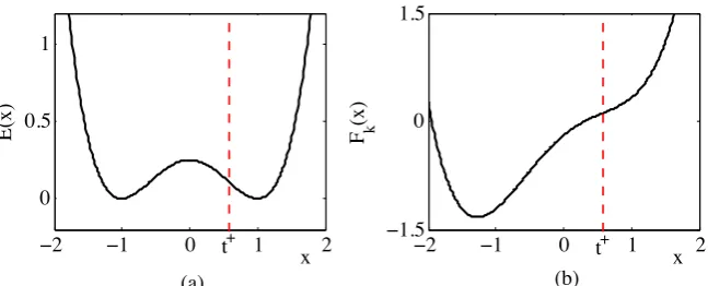
Figure 1. (a) Double-well energy defined in (14). (b) The auxiliary functional Fk(x) with xk = t+h; cf. §3.3. The second turning point
t−h =−t+h is an admissible descent step forFk, hence the dimer method can potentially cycle.
Proof. The Rotation Algorithm employed in step (3) of Linesearch Dimer Algo-rithm terminates for any starting guess due to the fact that it is a steepest de-scent algorithm on a Stiefel manifold (the unit sphere) with a backtracking line-search employing the Armijo condition [24]. Convergence of this iteration to a critical point is well known [1, Chap.4]. The loop (6,7) terminates after a fi-nite number of iterations [20] since p is a descent direction for Fk ∈ C4, that is,
Fk(xk+αp) =Fk(xk)−αkpk2+O(α2).
Remark 5. The two basic backtracking linesearch loops (5)–(8) and (11)–(12) can (and should) be replaced with more effective linesearch routines in practise, in particular choosing more effective initial guesses for the steps and using polynomial interpolation to compute linesearch steps. However, the discussion in§3.3 indicates
that a Wolfe-type termination criterion might be inappropriate.
3.3. Failure of global convergence. The modifications of the original dimer al-gorithms that we have in the Linesearch Dimer Algorithm would, in the case of optimisation, yield a globally convergent scheme. Unfortunately, this is not the case in saddle search. To see this, consider a one-dimensional double-well example,
E(x) = 1 4(1−x
2)2 = 1 4x
4− 1 2x
2+1
4; (14)
cf. Figure 1(a). There are only two possible (equivalent) dimer orientationv =±1, and therefore the rotation steps in Linesearch Dimer Algorithm are ignored. We always take v = 1 without loss of generality. The translation search direction at step k is always given by p = −(1−2)∇xEh(xk,1) = ∇xEh(xk,1), i.e., an ascent direction.
It is easy to see that x∗ = 0 is an index-1 saddle (i.e., a maximum), and that
there are two turning points t± = ±3−1/2. Thus, there exist “discrete turning points” t±h = ±3−1/2 +O(h2) such that λ(t±
h) = 0, where λ(x) = Hh(x; 1) ·1 = 1
2h2(E 0
(x+h)−E0(x−h)).
Suppose that we have an iterate xk =t+h, then the translation search direction is
p+ =∇
xEh(t+h,1)<0. Since Eh(t−h,1) = Eh(t+h,1) it follows that
Fk(t−h) = Eh(t−h,1)−2p +(t−
h −t +
Thus, for Θ sufficiently small, the update xk+1 =t−h satisfies all the conditions for termination of the loop (11)–(12) in Linesearch Dimer Algorithm. See also Figure 1 (b), whereFk is visualised.
We therefore conclude that our newly proposed variant of the dimer algorithm does not exclude cycling behaviour. We also remark that the example is not ex-clusively one-dimensional, but that analogous constructions can be readily made in any dimension.
3.4. Local convergence. We now establish a local convergence result.
Theorem 6. Let (x∗, v∗, λ∗)be an index-1 saddle, let (xh, vh, λh)denote the dimer
saddle associated with (x∗, v∗, λ∗) (cf. Theorem 2) and let xk, vk be the iterates
generated by the Linesearch Dimer Algorithm. Then there exist r, h0, C > 0 and γ ∈ (0,1) such that, for x0 ∈ Br(x∗), v−1 ∈ Br(v∗)∩SX and h ≤ h0, one of the
following alternatives are true:
(i) If ∇xEh(xk, vk−1) = 0 for some k ∈N, then kxk−xhk ≤Ch2. (ii) If ∇xEh(xk, vk−1)6= 0 for all k ∈N, then
kxk−xhk+kvk−vhk ≤Cγk kx0−xhk+h2kv−1−vhk
. (15)
Sketch of proof. Case (i) merely serves to exclude an unlikely situation, in which the Rotation algorithm is ill-defined. We do not discuss this case here, but treat it in §A.4.4. In the following assume Case (ii).
0. Let rk = kxk−xhk and sk := kvk−vhk. We recall basic contraction results for Armijo-based linesearch methods both in a general Hilbert space and for iterates constrained to lie on the unit sphere in§A.3.
1. As a first proper step we establish that, under the termination criterion k(1− vk⊗vk)Hh(xk;vk)k ≤ k∇xEh(xk, vk−1)k for the rotation step, it follows that sk .
rk+h2sk−1. This is proven in Lemma 15 and Lemma 16.
2. Next, we use this result to establish that there exists a local minimizer yk of
Fk satisfying kyk−xhk.rk2+h2rk+h4sk−1. This is established in Lemma 17. 3. The linesearch procedure and the upper bound on the step length ensure that the step of xk to xk+1 contracts towards yk, that is, kxk+1−ykk∗ ≤ γ∗kxk−ykk∗
for someγ∗ ∈(0,1) and k · k∗ the energy norm induced by (I−2v∗⊗v∗)∇2E(x∗)≈
∇2F
k(yk). This is obtained in Lemma 18.
4. The three preceding steps can then be combined to establish that, forr0, s−1, h sufficiently small, there exists a constantγ3 ∈(γ∗,1) such that
rk∗+1+h2sk ≤γ3(r∗k+h2sk−1), (16)
where r∗k := kxk −xhk∗. This contraction result readily implies the result of the
theorem.
The complete proof is given in §A.4.
4. Numerical Tests
deviates from the theoretical formulations of the Simple Dimer Algorithm and the Linesearch Dimer Algorithm.
In all cases the underlying space isX =RN for some N ∈
N. The main deviation from the algorithms stated in §2.2 and §3.2 is that we admit inner products that may change from one step to another,
kuk=puTM
ku, and u·v =uTMkv,
where Mk is symmetric and positive definite. That is, our implementation is a
variable metric variant; see also Remark 8 below.
Let E ∈ C4(X) =C4(RN), and let ∇0 denote the standard gradient and ⊗0 the
standard tensor product (i.e., the gradient and tensor products with respect to the
`2-norm), then the gradient and tensor products in step k become
∇E(x) = Mk−1∇0E(x), and (v ⊗v)∇E(x) = (v⊗0v)∇0E(x).
The variable metric variant of the Simple Dimer Algorithm, augmented with a ter-mination criterion, is given below. Note that here the rotation step is performed by a tangential descent step followed by a projection, rather than a step on the manifold.
Simple Dimer Algorithm (VM):
(1) Input: x0, v0 ∈X, h >0,α, β >0,TOLx,TOLv >0;k := 0; (2) While kMk−1/2∇0
xEh(xk, vk)k`2 >TOLx
. or k(Mk−1/2−Mk1/2vk⊗0vk)h−2∇0vEh(xk, vk)k`2 >TOLv do %% Metric %%
(3) Compute a spd matrix Mk ∈RN×N; (4) vk:=vk/kM
1/2 k vkk`2;
(5) vk+1 :=vk−β(Mk−1−vk⊗vk)h−2∇v0Eh(xk, vk) (6) xk+1 :=xk−α(Mk−1−2vk⊗vk)∇0xEh(xk, vk).
(7) k :=k+ 1
Remark 7. In our experiments we observe that the rotation residual decreases more quickly than the translation residual, hence the convergence criteria could be based on the translation residual only, without affecting the results.
Remark 8. Our analysis of both the Simple Dimer Algorithm and of the Linesearch Dimer Algorithm is readily extended to their variable metric variants, provided that the metric Mk at iterate k is a smooth function of the state, i.e.,
Mk = M(xk, vk), where M ∈ C2(Br(x∗)×SX;L(X)), for some r > 0. This is the case in all examples that we consider below. A more general convergence theory, e.g., employing quasi-Newton type Hessian updates requires additional work.
Analogous modifications are made to the Linesearch Dimer Algorithm. The aux-iliary functionalFk now reads
Fk(x) =Eh(x;vk)−2 vTk∇
0
xEh(xk, vk)
vkTMk(x−xk)
+λk vTkMk(x−xk)
2 ,
λk=h−2vTk∇
0
vEh(xk, vk),
∇0xEh(x, v) = 12 ∇0E(x+hv) +∇0E(x−hv)
,
∇0vEh(x, v) = h2 ∇0E(x+hv)− ∇0E(x−hv)
where we recall that∇0 denotes the standard gradient (i.e., the gradient with respect
to the`2-norm). See Remark 9 on additional improvements.
Linesearch Dimer Algorithm (VM):
(1) Input: x0, v0 ∈X, h >0,TOLx,TOLv >0; k := 0
(2) While kMk−1/2∇0
xEh(xk, vk)k`2 >TOLx
%% Metric %%
(3) Compute a spd matrix Mk ∈RN×N (4) v0k:=vk/kM
1/2 k vk−1k
%% Rotation %%
(5) [vk+1, β] := Rotation (VM)[xk, vk0, β, Mk]
%% Translation %%
(6) pM :=−(Mk−1−2vk+1⊗vk+1)∇0xEh(xk;vk+1) (7) α := min(αmax,2α)
(8) While (Fk(xk+αpM)> Fk(xk)−ΘαpTMMkpM)
. or (kMk1/2(Mk−1−vk+1⊗vk+1)h−2∇0vEh(xk+αpM;vk+1)k`2 >
. ΨkMk1/2(Mk−1−vk+1⊗vk+1)h−2∇0vEh(xk;vk+1)k`2) do
(9) α :=α/2
(10) xk+1 :=xk+αpM (11) k :=k+ 1
Rotation (VM):
(1) Input: x, v, β, Mk
Parameters: TOL = max(kMk−1/2∇0
xEh(x, v)k`2,TOLv), Θ∈(0,1), βmax;
(2) While kMk1/2(Mk−1−v ⊗v)h−2∇0
vEh(x;v)k>TOL do (3) s :=−(Mk−1−v⊗v)h−2∇0
vEh(x;v) (4) t :=kMk1/2sk`2; β := min(βmax,2β)
(5) vβ := cos(tβ)v+ sin(tβ)t−1s
(6) While Eh(x, vβ)>Eh(x, v)−Θβt2 do
(7) β :=β/2
(8) v :=vβ (9) Output: v, β
Remark 9. A modification that can give significant performance gains is to employ a different heuristic for the initial guess ofαin Step (7) of Linesearch Dimer Algorithm (VM): With pM,k :=−(Mk−1 −2vk⊗vk)∇0xEh(xk;vk) and pI,k :=−(I− 2vk⊗vk)∇0xEh(xk, vk) let, for k ≥ 2, γk := (pM,k−1 ·0 pI,k−1)/(pM,k·0 pI,k), then for
k≥2 we replace Step (7) with
α := min avg(γmax(2,k−4), . . . , γk),2α, αmax).
An analogous modification can be made for the rotation algorithm.
In all numerical tests we use the following parameters: h = 10−3, Θ = √0.1, TOLx = 10−5, TOLv = 10−1, α
• h should be small enough such that the dimer saddle is sufficiently close to the true saddle (with respect to the length scales of the given problem), while large enough that numerical robustness does not become a problem for the rotation. In all our tests, h= 10−3 was a good compromise.
• Θ should be sufficiently large (though, ≤1/2) to ensure that the linesearch method finds steps which give a large decrease in dimer energy. It is often chosen much smaller than our choice of Θ = √0.1 to immediately accept steps that make some progress. Our experience is that, with preconditioned search direction, our more stringent choice gives better performance as it leads to an improved initial steplength guess for the next iteration.
• The choice of TOLx simply controls the desired level of convergence to the dimer saddle.
• The parameter TOLv should be chosen as weakly as possible such that either algorithm converges to the saddle. In the Linesearch Dimer Algorithm (VM) rotations are performed such that the rotation residual is at least as good as the translation residual until it moves below this value. Subsequent trans-lations may increase the rotation residual such that further applications of the rotation algorithm are needed. In practise this means that the rotation algorithm is performed at every iteration of the Linesearch Dimer Algorithm (VM) for the first few steps, then only sporadically or not at all once the rotation residual reaches TOLv. The use of this parameter then decreases the overall number of gradient evaluations needed to find the dimer saddle, by only performing the rotation as necessary.
• The maximum step αmax should principally be chosen such that the dimer cannot translate into non-physical regimes for the given problem.
• The parameter Ψ should be chosen>1 and restricts the translation step from moving the dimer to a point where it becomes too badly orientated. In our numerical tests this parameter is set sufficiently large that this termination criteria for the translation never occurs (the translation always terminates by finding a sufficient decrease in the auxiliary functional Fk).
Remark 10. We observe during numerical testing that the rotation component of the linesearch dimer is somewhat vulnerable to rounding error in the objective functionE. As the dimer becomes increasingly well orientated, ∇E becomes almost orthogonal to the dimer orientation and any small rotation may result in a zero change (to numerical precision) in the dimer energy. In the numerical examples presented in this section, this never occurs since we use a relatively high value for TOLv, that is the rotation is only ever weakly converged. In our examples this is sufficient for the the dimer to converge to the saddle. If a stronger level of convergence were required, another technique should be used to improve the rotation residual further, such as changing to a gradient based method or simply making fixed steps. This could, for example, be performed in a post-processing step (cf. Remark
1 on post-processing x).
−2 0 2
−3
−2
−1 0 1 2 3
(B)
−10 −5 0 5 10
−10
−5 0 5 10
[image:14.595.153.447.88.245.2](A)
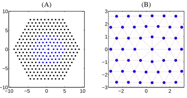
Figure 2. Initial configuration of the atoms in the vacancy dif-fusion problem (Test 1) . Black squares are fixed atoms while blue circles are atoms which move freely. (A) The initial dimer orientation is selected so that the translated atom has an orientation along the
y = 0 direction, and is zero for all other atoms. (B) The DelaunayTk triangulation used for the connectivity norm.
−10 −5 0 5 10
−10 −5 0 5 10
(A)
−2 0 2
−3 −2 −1 0 1 2 3
(B)
Figure 3. Final configuration of the atoms in the vacancy diffusion problem (Test 1). Black squares are fixed atoms while blue circles are atoms which move freely. (A) In the final configuration an atom moves to the midpoint between two ‘basins’. (B) The Delaunay triangulation Tk used for the connectivity norm.
The energy function is given by the simple Morse potential,
E({xi}) =
X
i,j
V(kxi−xjk2), V(r) =e−2a(r−1)−2e−a(r−1), (17)
with stiffness parameter a= 4.
[image:14.595.150.449.374.530.2]0 200 400 10−6
10−4 10−2 100 102
#∇Eh
∥∇ x Eh ( x, v ) ∥ (A)
nA= 23
nA= 69
nA= 139
nA= 233
0 100 200 300
10−6 10−4 10−2 100 102 niter ∥∇ x Eh ( x, v ) ∥ (B)
nA= 23
nA= 69
nA= 139
nA= 233
0 50 100 150
10−6 10−4 10−2 100 102
#∇Eh
∥∇ x Eh ( x, v ) ∥ (C)
nA= 23
nA= 69
nA= 139
nA= 233
0 20 40 60
10−6 10−4 10−2 100 niter ∥∇ x Eh ( x, v ) ∥ (D)
nA= 23
nA= 69
nA= 139
[image:15.595.131.459.99.409.2]nA= 233
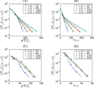
Figure 4. Convergence of the linesearch dimer to the saddle in the vacancy diffusion problem (Test 1) with (A),(B) the `2 norm and (C),(D) connectivity norm versus the number of force evaluations and dimer iterations for increasing numbers of free atoms.
triangulation of the atomistic positions (Figure 2(B))
hMku, ui=
Z
|∇ITku| 2
,
where Tk is the triangulation depicted in the figure and ITk the associated nodal interpolant.
Figure 4 demonstrates the convergence to the saddle with different numbers of free atoms nA (giving different dimensionality of the system) in the two norms for the linesearch dimer. We can also observe the benefit of the linesearch vs a simple dimer scheme when using the connectivity norm (Figure 5). The linesearch dimer selects very efficient stepsizes with no a-priori information, while the simple dimer method might exhibit either slow convergence, or no convergence, if the fixed steps are poorly chosen.
4.3. Test 2: A Phase Field Example. Our second example is based on a simple phase field model where the global energy is given by,
E(u) =
Z
Ω
2|∇u| 2
+ 1
2(u 2−
0 200 400 600 10−6
10−4 10−2 100 102
#∇Eh
∥∇
x
Eh
(
x,
v
)
∥
(A)
0 200 400 600
10−6 10−4 10−2 100 102
niter
∥∇
x
Eh
(
x,
v
)
∥
(B)
linesearch
α,β= 0.001
α,β= 0.005
α,β= 0.01
α,β= 0.05
linesearch
α,β= 0.001
α,β= 0.005
α,β= 0.01
[image:16.595.133.469.96.257.2]α,β= 0.05
Figure 5. Convergence of the linesearch dimer vs the simple dimer method for Test 1 (vacancy), for several choices of the simple dimer step sizes, with nA= 69, using the connectivity norm as a precondi-tioner.
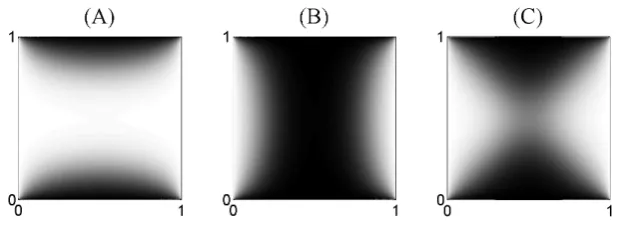
Figure 6. Minima (A,B) and saddle point (C) of the phase field problem (Test 2) with = 1/10. The shading is linearly interpolated between white(-1) and black(1).
where Ω = (0,1)2, and the boundary conditions are,
u(x) =
−1, x1 ∈ {0,1} 1, x2 ∈ {0,1}.
(19)
There are 2 minima of such an energy, these are given in Figure 6(A),(B). The saddle between these two minima is given in Figure 6(C).
A possible choice for a preconditioner for this system is a stabilized Laplacian,
P =∆ + 1
I. (20)
[image:16.595.147.457.350.464.2]0 10 20 30 40 10−1.05
10−1.04 10−1.03
#∇Eh ∥∇ x Eh ( x, v ) ∥ (A)
α,β=1.00e-01
α,β=1.00e-02
α,β=1.00e-03
α,β=1.00e-04
0 10 20 30 40
10−4 10−2 100 102 #∇Eh ∥∇ x Eh ( x, v ) ∥ (B)
α,β=1.00e-02
α,β=5.62e-02
α,β=3.16e-01
[image:17.595.114.471.82.252.2]α,β=1.78e+00
Figure 7. Convergence of the simple dimer to the saddle in the phase field problem (Test 2) with (A) the `2 metric and (B) the sta-bilized Laplacian metric where = 1/10 for a triangulation with 3485 degrees of freedom.
In Figure 7 we demonstrate the necessity of using a preconditioner to solve this problem using the simple dimer method. When using the preconditioner (20), the algorithm performs well when the step size is chosen appropriately. We observe the expected behaviour, that there exists an optimal step size where convergence is fastest, and beyond that step size the dimer diverges. In fact we observe that the stabilized Laplacian metric is so effective, that the optimal step size seems very close to the unit step. If the `2 norm (identity preconditioner) is used then for all step sizes tested the dimer diverges, indicating that at best a very small step would need to be chosen for convergence.
In Figure 8 we demonstrate that the used of the scaled Laplacian metric for different system sizes. We observe that the use of this metric gives almost perfect scale invariance.
0 10 20 30
10−6
10−4
10−2
100
#∇Eh
∥∇ x Eh ( x, v ) ∥ (A)
#DOF = 845 #DOF = 3485 #DOF = 14165
0 5 10 15 20
10−6
10−4
10−2
100 niter ∥∇ x Eh ( x, v ) ∥ (B)
#DOF = 845 #DOF = 3485 #DOF = 14165
[image:17.595.122.472.541.705.2]0 10 20 30 10−6
10−4 10−2 100 102
#∇Eh
∥∇ x Eh ( x, v ) ∥ (A)
ϵ= 1/10 ϵ= 1/15 ϵ= 1/20
0 10 20 30 10−6
10−4 10−2 100 102 niter ∥∇ x Eh ( x, v ) ∥ (B)
ϵ= 1/10 ϵ= 1/15 ϵ= 1/20
0 50 100
10−6 10−4 10−2 100 102
#∇Eh
∥∇ x Eh ( x, v ) ∥ (C)
ϵ= 1/10 ϵ= 1/15 ϵ= 1/20
0 10 20 30 10−6
10−4 10−2 100 102 niter ∥∇ x Eh ( x, v ) ∥ (D)
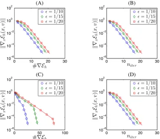
[image:18.595.131.456.94.377.2]ϵ= 1/10 ϵ= 1/15 ϵ= 1/20
Figure 9. Convergence to the saddle in the phase field problem (Test 2) using the stabilized Laplacian metric with (A),(B) the simple dimer with unit step length and (C),(D) the linesearch dimer for a tri-angulation with 2405,9805,22205 degrees of freedom for the respective choices of .
In Figure 9 we give the results of applying the simple and linesearch dimers with varying ; the coarseness of the discretization in each experiment is chosen such that ∆x ≈ /5. In some of these cases the linesearch dimer fails due to rounding error. Specifically, due to rounding error in the naive implementation of the energy function (simple summation over the elements), the translation step fails to find a sufficient decrease in the dimer energy, the step size selected shrinks to zero (to rounding error) and the method stagnates. In order to correct this a more robust method of evaluating the energy or a more advanced optimization algorithm should be implemented which can either choose better linesearch directions or more robustly deal with numerically zero energy changes.
5. Conclusions
We have described a dimer method for finding a saddle point in which the dimer length h is not required to shrink to zero, but which converges to a point that lies within O(h2) of a saddle. We have enhanced this algorithm with a lineasearch to improve its robustness and efficiency, and use the observation that the dimer method may be formulated and applied in a general Hilbert space to allow preconditioning that improves the method’s efficiency. The linesearch uses a local merit function. Unfortunately our particular merit function may not lead to global convergence of the iterates, and it is an open question as to whether there is another merit function that ensures global convergence. We have illustrated the positive effects of our algorithms on two realistic examples.
Appendix A. Proofs
We remark that all proofs in this section are independent of the choice of norm k · k(not necessarily the `2-norm) and are hence valid for the preconditioned version of the algorithm.
A.1. Proof of Proposition 2. We prove the result using the inverse function the-orem. We write (9) as F(xh, vh, λh) = 0 and show that kF(x∗, v∗, λ∗)k ≤ Ch2 and
that ∇F(x∗, v∗, λ∗) is an isomorphism with bounds independent of h. The inverse
function theorem then yields the stated result.
Residual estimate. Let the residual components be
rx :=Fx(x∗, v∗, λ∗) = ∇xEh(x∗, v∗),
rv :=Fv(x∗, v∗, λ∗) =h−2∇vEh(x∗, v∗)−λ∗v∗,
rλ :=Fλ(x∗, v∗, λ∗) = 12(kv∗k2−1).
Then (2) and (4) imply thatrx, rv, rλ =O(h2) and hencekF(x∗, v∗, λ∗)k ≤Ch2. Stability. ∇F(x∗, v∗, λ∗) can be written in the form, using
∇F(x∗, v∗, λ∗) =
∇2
xEh(x∗, v∗) ∇v∇xEh(x∗, v∗) 0 h−2∇v∇xEh(x∗, v∗) h−2∇2vEh(x∗, v∗)−λ∗I −v∗
0 −v∗T 0
=
∇2E(x
∗) 0 0
∇3E(x
∗)·v∗ ∇2E(x∗)−λ∗I −v∗
0 vT
∗ 0
+O(h2) =:A+O(h2),
where we used (3), (4) and (6). By assumption, ∇2E(x
∗) is an isomorphism on X.
Since, also by assumption, λ∗ is a simple eigenvalue, the block
∇2E(x
∗)−λ∗I −v∗
v∗T 0
(21)
is an isomorphism on X×R as well. Thus, A is an isomorphism on X×X ×R and consequently, for allh sufficiently small, ∇F(x∗, v∗, λ∗) = A+O(h2) is also an
isomorphism, with a uniform bound on its inverse.
A.2. Proof of Theorem 3. Fix r and h0 sufficiently small so that Theorem 2 applies. Letek :=xk−xh, fk :=vk−vh and rk:=
p
kekk2 +kfkk2, so that trivially kekk ≤rk and kfkk ≤rk.
Lemma 11. Letp:=−(I−2vk⊗vk)∇xEh(xk, vk)ands:=−(I−vk⊗vk)Hh(xk;vk),
then, under the assumptions of Theorem 3,
p=−Aek+O(rk2+h 2
rk), and (22)
s=−Bek−Cfk+O(rk2+h 2r
k), (23)
where the operatorsAandC are defined in (12)andB is a bounded linear operator.
Proof. We begin by noting the elementary identities which are easy to establish:
∇xEh(xk, vk)− ∇xEh(xh, vh) = O(rk),
vk⊗vk−vh⊗vh =O(rk), (24)
∇2
xEh(xh, vh) = ∇2E(xh) +O(h2) = ∇2E(x∗) +O(h2)
Using the identities (24), as well as (2), (6), we can expand
p=−(I−2vk⊗vk) ∇xEh(xk, vk)− ∇xEh(xh, vh)
,
=−(I−2vh⊗vh) ∇2xEh(xh, vh)ek+∇x∇vEh(xh, vh)fk
+O(r2k)
=−(I−2vh⊗vh)∇2E(xh)ek+O(r2k+h 2r
k)
=−(I−2v∗⊗v∗)∇2E(x∗)ek+O(r2k+h 2r
k)
=−Aek+O(rk2+h2rk).
To prove (23), we first note that, with kvk= 1,
Hh(x;v) =−
Z 1
−1
∇2E(x+thv) dt v =∇2E(x)v+O(h2),
Hh(xh;vh) =∇2E(xh)vh+O(h2) = ∇2E(x∗)v∗+O(h2),
Hh(xk;vk)−Hh(xh;vh) =− Z 1
−1
∇2E(xk+thvk)− ∇2E(xh+thvh)
dt vk
+−
Z 1
−1
∇2E(x
h+thvh) dt(vk−vh)
=−
Z 1
−1
∇3E(xh+thvh)
(xk−xh) +th(vk−vh)
dtvh
+∇2E(x
∗)(vk−vh) +O(r2k+h 2r
k)
= (∇3E(x
where we interpret∇3E(x)·v ∈L(X) via the actionw·((∇3E(x)·v)z) = lim
t→0t−1w· ((∇2E(x+tv)− ∇2E(x))z). Finally, we also have
(vk⊗vk−vh⊗vh)Hh(xh;vh) = (vk⊗vk−vh⊗vh)∇2E(x∗)v∗+O(h2rk)
=λ∗(vk⊗vk−vh⊗vh)v∗+O(h2rk)
=λ∗(vk⊗vk−vh⊗vh)vh+O(h2rk)
=λ∗(vk−vh) +λ∗vk((vk−vh)·vh) +O(h2rk)
=λ∗fk+O(r2k+h 2r
k).
In the very last line we also used the fact that vk·vh−1 = −21kvk−vhk2. Using these identities, we can compute
s=−(I−vk⊗vk)Hh(xk;vk)
= (I−vh⊗vh)Hh(xh;vh)−(I−vk⊗vk)Hh(xk;vk)
=−(I−vk⊗vk) Hh(xk;vk)−Hh(xh;vh)
+ (vk⊗vk−vh⊗vh)Hh(xh;vh)
=−(I−vk⊗vk) (∇3E(x∗)v∗)ek+∇2E(x∗)fk
+O(h2rk+r2k)
+λ∗fk+O(r2k+h 2r
k)
=:−Bek+
λ∗I−(I−v∗⊗v∗)∇2E(x∗)
fk+O(r2k+h 2r
k)
=−Bek−Cfk+O(rk2+h2rk).
From Lemma 11 it follows in particular that s=O(rk). Hence, Taylor expansions of sine and cosine in the identity
vk+1 = cos kskβk)vk+ sin(kskβk)kssk,
yield
fk+1 =fk+βks+O(βk2s 2 k)
Using Lemma 11, the identityek+1 =ek+αkp, and the fact thatβk is bounded, we therefore obtain identity (12) in the proof outline in §2.4.
Since A, C are positive definite, it follows that, for αk, βk sufficiently small, the spectrum of the operator
I−
αkA 0
βkB βkC
lies in some interval [0, µ] for µ < 1. Thus, for fixed steps αk ≡α and βk ≡β, (11) follows from standard linearised stability arguments for discrete dynamical systems. The straighforward generalisation to non-uniform steps is presented in [9].
A.3. Contraction of steepest descent with linesearch. In the section following this one, we will use statements about the steepest descent method with backtracking that we suspect are well known. Since we have been unable to find precisely the statement that we require, we state both below, and give complete proofs in [9].
Lemma 12. Let X be a Hilbert space, F ∈C3(X), and x
∗ ∈X with ∇F(x∗) = 0 and ∇2F(x
∗) positive definite, i.e., u·(∇2F(x∗)u)≥µkuk2 for µ > 0. Let kuk2∗ := u·(∇2F(x
Then, there exists r >0 and γ ∈(0,1), depending only on α,α, µ,¯ k∇jF(x)k for
x∈B1(x∗), such that, for allα ∈[α,α¯]and for all x∈Br(x∗) satisfying the Armijo condition
F(x−α∇F(x))≤F(x)−Θαk∇F(x)k2,
we have
[x−α∇F(x)]−x∗
∗ ≤γkx−x∗k∗.
We now generalize the foregoing result to steepest descent on the unit sphere. Convergence results for many methods on manifolds are given by [1, Chap.4]. See specifically [1, Thm.4.5.6] and [2].
Lemma 13. Let X be a Hilbert space, Pv :=v⊗v and Pv0 :=I −Pv for v ∈SX.
Let F ∈C3(X),
g(v) :=Pv0∇F(v) and H(v) :=Pv0∇2F(v)P0
v− ∇F(v)·v
I.
We assume that there existsv∗ ∈SX and µ >0 such that
g(v∗) = 0 and u· H(v∗)u
≥µkuk2 ∀u∈X. (25)
Let kuk∗ := p
u·(H(v∗)u).
Let α >¯ 0, Θ∈(0,1), and for v ∈SX and α∈R, denote
vα := cos αkg(v)k
v−sin αkg(v)k g(v) kg(v)k.
Then, there exists r >0 such that, for all v ∈Br(v∗)∩SX and α∈(0,α¯] satisfying
the Armijo condition
F(vα)≤F(v)−Θαkg(v)k2,
there exists a constantγ(α)∈[0,1) such that
vα−v∗
∗ ≤γ(α)kv−v∗k∗.
The contraction factorγ(α)depends onα, µand onk∇jF(x)k, x∈B
1(v∗). More-over, for anyα ∈(0,α¯], supα∈[α,α¯]γ(α)<1.
A.4. Proof of Theorem 6. Throughout this proof, we fix an index-1 saddle (x∗, v∗, λ∗),
and assume thath0 is small enough so that Proposition 2 ensures the existence of a dimer saddle (xh, vh, λh) in anO(h2) neighbourhood of (x∗, v∗, λ∗).
Until we state otherwise (namely, in §A.4.4) we assume that ∇xEh(xk, vk−1)6= 0 for all k. In particular, the Linesearch Dimer Algorithm is then well-defined and produces a sequence of iterates (xk, vk)k∈N. That is, we are in Case (ii) of Theorem
6. The alternative, Case (i), is treated in §A.4.4.
A.4.1. Analysis of the rotation. We begin by establishing an auxiliary result con-cerning existence of minimisers of v 7→ Eh(x, v). Let
V(x) := arg min v∈SX
Eh(x, v),
Lemma 14. Let (x∗, v∗, λ∗) be an index-1 saddle, then there exist r > 0, h0 > 0
(chosen independently of one another) such that, for all x∈Br(x∗) andh∈(0, h0], V(x) is well-defined and moreover x7→V(x)∈C1(B
r(x∗)).
Proof. For r sufficiently small, if x ∈ Br(x∗) then ∇2E(x) also has index-1 saddle
structure and, if (λ, v) is the smallest eigenpair of ∇2E(x), then λ ≤ λ
∗/2 and
(∇2E(x)w)·w≥µ
∗/2kwk2 forw⊥v, whereµ∗ := infkwk=1,w⊥v∗(∇
2E(x
∗)w)·w >0.
(This statement is a straightforward consequence of the local Lipschitz continuity of ∇2E, which follows sinceE ∈C4(X).)
The statement of the Lemma is then proven similarly as Proposition 2, providedh0 is chosen sufficiently small (depending onλ∗, µ∗ and on derivatives ofE inB2r(x∗)).
TheC1-dependence ofV(x) on xis a consequence of the implicit function theorem.
Next, we obtain a bound on vk−vh in terms of xk−xh and the residual of vk.
Lemma 15. There exist r, h0, C1 > 0 such that, for h ∈ (0, h0], x ∈ Br(x∗) and v ∈Br(v∗) with kvk= 1, we have
kv −vhk ≤ 12C1 kx−xhk+
(I−v⊗v)Hh(x;v)
.
Proof. Let λ:=Hh(x;v)·v, then
Hh(xh;v) = λv+s, 1
2kvk 2 = 1
2,
(26)
where
s= Hh(xh;v)−Hh(x;v)
+ (I−v⊗v)Hh(x;v). Sincevh solves (26) with s= 0, and since
ksk ≤C2 kx−xhk+k(I −v ⊗v)Hh(x;v)k
,
the stated result follows from the Lipschitz continuity ofHh(·;v) and an application of the inverse function theorem, in a similar spirit as the proof in §A.1.
Next, we present a result ensuring that the rotation step of Algorithm 3 not only terminates but also produces a new dimer orientation vk which remains in a small neighbourhood of the “exact” orientationvh.
Lemma 16. There existr, h0, C2 >0, C3 ≥1such that, ifh∈(0, h0],xk ∈Br(x∗), vk−1 ∈ BC3r(v∗), kvk−1k = 1, then Step (3) of the Linesearch Dimer Algorithm terminates with outputs vk ∈BC3r(v∗), kvkk= 1, βk >0, satisfing
kvk−vhk ≤C2 kxk−xhk+h2kvk−1−vhk
. (27)
Proof. Let G(v) := h−2(E
h(xk;v)− Eh(xk;V(xk))), then each step of the Rotation Algorithm is a steepest descent step of G on the manifold SX. We need to ensure that these iterations do not “escape” from the minimiser V(xk) (cf. Lemma 14).
Lemma 13 (with F(v) = G(v) and v∗ = V(xk)) implies that each such step is a contraction towardsV(xk) with respect to the normk · kH induced by the operator
H := (I−V ⊗V)∇2G(V)(I−V ⊗V)−(∇G(V)·V)I,
To see that the latter is indeed true, we recall from (4) and (5) that
∇G(V) =∇2E(x
k)V +O(h2) and ∇2G(V) =∇2E(xk) +O(h2)
and from Proposition 2 and Lemma 14 that
V(xk) = v∗+O(h2+r), (28)
from which we can deduce that
H = (I−v∗⊗v∗)∇2E(x∗)(I−v∗⊗v∗)− (∇2E(x∗)v∗)·v∗
I+O(h2+r)
= (I−v∗⊗v∗)∇2E(x∗)−λ∗I+O(h2+r).
Since (x∗, v∗, λ∗) is an index-1 saddle, (I −v∗ ⊗v∗)∇2E(x∗) is positive definite in
{v∗}⊥, andλ∗ <0. Thus, forh, rsufficiently small,H is positive definite as required.
From Lemma 13, it follows that all iterates vk(j) of the Rotation Algorithm sat-isfy kv(kj)−V(xk)kH ≤ kvk−1 −V(xk)kH. Since the eigenvalues of H are uniformly bounded below and above, the norms k · kH,k · k are equivalent, and hence in par-ticular
kvk−V(xk)k ≤C7kvk−1−V(xk)k ≤C7(kvk−1 −v∗k+kV(xk)−v∗k) =O(h2+r)
for some constant C7 > 0, since vk−1 ∈ BC3r(v∗) and using (28). Combining this
with (28) and choosing h20 ≤r, we deduce that the Rotation Algorithm terminates with an iterate vk such that
kv∗−vkk ≤ kv∗−V(xk)k+kvk−V(xk)k ≤C4r
for some constant that depends only on r but is independent of vk−1 and remains bounded as r→0.
At termination the Rotation Algorithm guarantees the estimate
(I −vk⊗vk)Hh(xk;vk)
≤ k∇xEh(xk, vk−1)k.
We setxt= (1−t)xh+txk,vt =vh+tvk−1 and expand
∇xEh(xk, vk−1)
=
Z 1
0
∇2
xEh(xt, vt)(xk−xh) +∇v∇xEh(xt, vt)(vk−1−vh)
dt
≤C20 kxk−xhk+h2kvk−1−vhk
.
Combined with Lemma 15 this yields the estimate (27).
The statement that vk ∈ BC3r(v∗) (instead of only BC4r(v∗)) is an immediate
consequence of (27) by ensuring thatC3 ≥C2+C3h2+C0h4, wherekvh−v∗k ≤C0h2
for all h ≤ h0 from Proposition 2. While there is an interdependence between C3 and C2, for r and h0 sufficiently small, this is clearly achievable.
A.4.2. Analysis of the translation. We first establish the existence of a minimiser of the auxiliary functionalFk under the conditions ensured by the rotation step of the Linesearch Dimer Algorithm.
Lemma 17. Under the conditions of Lemma 16, possibly after choosing a smaller r, h0, there exists a constant C4 >0, such that the functional Fk defined in (13) has
a unique minimiser yk ∈Br(x∗) satisfying
kyk−xhk ≤C4(rk2+h 2r
Proof. We begin by estimating the residual
∇Fk(xh) = ∇xEh(xh, vk)−2(∇xEh(xk, vk)·vk)vk+ 2λk((xk−xh)·vk)vk,
whereλk=Hh(xk;vk)·vk. We consider each constituent term in this expression in turn; we expand about (xh, vh), and use the identities (7), (9) and (24) This gives
vk=vh+O(sk)
∇xEh(xh, vk) = ∇x∇vEh(xh, vh)(vk−vh) +O(s2k)
∇xEh(xk, vk) = ∇2xEh(xh, vh)(xk−xh) +∇x∇vEh(xh, vh)(vk−vh)
+O(r2k) +O(s2k)
=∇2xEh(xh, vh)(xk−xh) +O(h2sk) +O(rk2) +O(s 2 k),
∇xEh(xk, vk)·vkvk= (∇2xEh(xh, vh)(xk−xh) +∇x∇vEh(xh, vh)(vk−vh))·vhvh
+O(r2k) +O(s2k) +O(rksk)
=∇2
xEh(xh, vh)(xk−xh)·vhvh
+O(h2sk) +O(r2k) +O(s 2
k) +O(rksk)
Hh(xk;vk) = Hh(xh;vh) +O(rk) +O(sk)
λk=λh+vk·Hh(xk;vk)−vh·Hh(xh;vh) = λh+O(rk) +O(sk)
λk((xk−xh)·vk)vk= (λh+O(rk) +O(sk))((xk−xh)·vk)vk
=λh((xk−xh)·vh)vh+O(rk2) +O(rksk).
Thus since (10) and our assumption thatvk−1 ∈BC3r(v∗) ensure that sk−1 =O(1 +
h2
0), while (27) implies thatsk =O(rk) +O(h2sk−1), we combine the above to obtain
∇Fk(xh) = −2
(∇2
xEh(xh, vh)(xk−xh))·vh
vh+ 2λh((xk−xh)·vh)vh
+O r2k+h2rk+h4sk−1
,
Next, we note that, by definition of Eh, ∇2
xEh(xh, vh)vh = ∇2E(xh)vh+O(h2), and thus from (4) that∇2
xEh(xh, vh)vh =Hh(xh;vh) +O(h2). Hence applying (9),
∇Fk(xh) = −2Hh(xh;vh)·(xk−xh) + 2λh(xk−xh)·vh
vh (30)
+O r2k+h2rk+h4sk−1
=O r2k+h2rk+h4sk−1
. (31)
Finally, we observe that∇2F
k(xh) is positive definite, since
∇2F
k(xh) =∇2xEh(xh, vk)−2λkvk⊗vk
=∇2
xEh(xh, vh)−2λhvh⊗vh+O(rk)
=∇2E(x∗)−2λ∗v∗⊗v∗+O(h2+rk), (32)
which immediately implies that, for r, h0 sufficiently small, ∇2Fk(xh) is an isomor-phism with uniformly bounded inverse.
Thus an application of the inverse function theorem to∇Fk atykusing (31) yields
the stated result.
We now turn towards analysing the linesearch for x. Recall the definition of the energy normkuk∗ :=
p
particular,
µ1/2kuk ≤ kuk∗ ≤ k∇2E(x∗)kkuk where µ:= min(−λ∗, µ∗)>0. (33)
Lemma 18. There exists r, h0, α∈(0, α0] andγ∗ ∈(0,1), such that, if h∈(0, h0], xk∈Br(x∗), vk ∈BC3r(v∗) and αk−1 ≥α, then
αk ≥α and kxk+1−ykk∗ ≤γ∗kxk−ykk∗,
where yk is the minimiser of Fk established in Lemma 17.
Proof. We begin by noting that, for any r >0, the norms k∇2F
k(x)k are uniformly bounded among all choices ofxk ∈Br(x∗),x∈Br+1(x∗). This is straightforward to
establish.
Therefore, there exists α > 0 such that, for xk ∈ Br(x∗) and for any α ∈(0,2α],
the conditions in Step (6) of the Linesearch Dimer Algorithm are met (this includes an Armijo condition for Fk) since ∇Fk is Lipschitz in a neighbourhood of xk [8, Thm.2.1]. It is no restriction of generality to requireα≤α0. In particular,αk≥α. For r, h0 sufficiently small, we have yk ∈ Br(x∗) as well. Upon choosing r
suffi-ciently small, u·(∇2Fk(y)u) ≥ µ/2kuk2 for all u ∈ X, y ∈ Br(x
∗). Thus, we can
apply Lemma 12 (with x∗ ≡ yk) to deduce that, for r sufficiently small, the step
xk+1 = xk−αk∇F(xk) is a contraction with a constant γ1 that is independent of xk, vk. That is,
(xk+1−yk)·
∇2Fk(yk)(xk+1−yk)
≤γ12(xk−yk)·
∇2Fk(yk)(xk−yk)
,
Recalling from (29) and (32) that ∇2F
k(yk) = (I −2v∗ ⊗v∗)∇2E(x∗) +O(r+h2)
we find that, forr, h0 sufficiently small,
kxk+1−ykk∗ ≤γ∗kxk−ykk∗, (34)
whereγ∗ ∈[γ1,1), again independent of xk, vk, but depending onr, h0.
A.4.3. Proof of Case (ii). We have assembled all prerequisites to complete the proof of Theorem 6, Case (ii).
Inspired by Lemma 18, our aim is to prove that, for r sufficiently small, there existsγ ∈(0,1) such that, for all j ≥0,
rj∗+h2sj−1 ≤γj(r∗0+h 2
s−1) =:γjt0, (35)
whereγ := 12(γ∗+ 1), r∗k:=kxk−xhk∗ and sk:=kvk−vhk.
A consequence of (35) would be that there exists a constantcsuch thatkxj−x∗k ≤ cr=: ˆr. Thus, under the assumptions of the Theorem, letr, h0be chosen sufficiently small so that Proposition 2, and Lemmas 15, 16, 17 and 18 apply with r replaced by ˆr.
We now begin the induction argument adding to (35) the conditions that
vj−1 ∈BC3r(v∗) and αj ≥α, (36)
whereC3 ≥1 is the constant from Lemma 16 and α the constant from Lemma 18. Clearly (35) and (36) hold forj = 0. Suppose that they hold for j = 0, . . . , k, where
k≥0.
Applying Lemma 18 we obtain the second condition in (36) for j =k+ 1, and in addition that
kxk+1−ykk∗ ≤γ∗kxk−ykk∗,
whereyk is the minimiser of Fk established in Lemma 17. Using (34), the fact that
γ∗ < 1 and Lemma 17 we therefore deduce that there exists a constant C5 which depends on C4 and on the norm-equivalence between k · k and k · k∗, such that
kxk+1−xhk∗ ≤ kxk+1−ykk∗+kyk−xhk∗
≤γ∗kxk−ykk∗+kyk−xhk∗
≤γ∗kxk−xhk∗+ 2kyk−xhk∗
≤(γ∗+C5h2+C5rk)kxk−xhk∗+C5h4kvk−1 −vhk.
Adding h2kv
k−vhkto both sides of the inequality and applying (27) and (33) we thus obtain
rk∗+1+h2sk ≤(γ∗+C5h2+C5rk)rk∗+h2sk+C5h4sk−1
≤ γ∗+C5h2+µ−1/2C2h2+C5(c+ 1)r
rk∗+ (C5+C2)h4sk−1.
Recalling thatγ = 12(γ∗+ 1), choosing h0, r sufficiently small, we obtain that
rk∗+1+h2sk≤γ(r∗k+h 2s
k−1).
This establishes (35) for j =k+ 1 and thus completes the induction argument. In summary, we have proven that (35) and (36) hold for all j ≥ 0. As a first consequence, we obtain thatrk :=kxk−xhk ≤µ−1/2k∇2E(x∗)kγk(r0+h2s−1) using (33), which in particular establishes the first part of (15).
To obtain a convergence rate for vk we combine (27) and (35), to obtain
kvk−vhk ≤C6(r∗k+h 2
sk−1)≤C6γkt0 ≤C6k∇2E(x∗)kγk(r0+h2s−1),
for a constant C6. Choosing C = 2 max(C6, µ−1/2)k∇2E(x∗)k completes the proof
of Theorem 6, Case (ii).
A.4.4. Proof of Case (i). The proof of Case (ii) establishes that, for as long as ∇xEh(xk, vk−1) 6= 0, the iterates are well-defined and kxk−xhk+kvk−vhk ≤ Cr for some suitable constant C. We now drop this assumption and instead suppose that, at the`th iterate,∇xEh(x`, v`−1) = 0. In this case, we can apply the following lemma.
Lemma 19. Let(x∗, v∗, λ∗)be an index-1 saddle, then there exist r, h0, C > 0such
that, for all h ∈(0, h0] and for all v ∈SX, there exists a unique xh,v ∈Br(x∗) such that∇xEh(xh,v, v) = 0. Moreover, kxh,v−xhk ≤Ch2.
Proof. This is an immediate corollary of (2) and the inverse function theorem.
Since kx`−xhk ≤Cr, Lemma 19 implies that, in fact kx`−xhk ≤C0h2 for some other constantsC0, provided that r, h are chosen sufficiently small.
References
[1] P.-A. Absil, R. Mahony, and R. Sepulchre. Optimization Algorithms on Matrix Manifolds. Princeton University Press, Princeton, USA, 2008.
[2] P.-A. Absil, R. Mahony, and J. Trumpf. An extrinsic look at the Riemannian Hessian. In F. Nielsen and F. Barbaresco, editors, Geometric Science of Information, number 8005 in Lecture Notes in Computer Science, pages 361–368, Heidelberg, Berlin, New York, 2013. Springer Verlag.
[3] A. Banerjee, N. Adams, J. Simons, and R. Shepard. Search for stationary points on surfaces. The Journal of Physical Chemistry, 89:52–57, 1985.
[4] G.T. Barkema and N. Mousseau. Event-based relaxation of continuous disordered systems. Physical Review Letters, 77:4358, 1996.
[5] G.T. Barkema and N. Mousseau. The activation-relation technique: an efficient algorithm for sampling energy landscapes.Computational Materials Science, 20(3–4):285–292, 2001. [6] E. Cances, F. Legoll, M.C. Marinica, K. Minoukadeh, and F. Willaime. Some improvements
of the activation-relaxation technique method for finding transition pathways on potential energy surfaces.The Journal of Chemical Physics, 130(114711), 2009.
[7] C.J. Cerjan and W.H. Miller. On finding transition states. Journal of Chemical Physics, 75:2800, 1981.
[8] N. I. M. Gould and S. Leyffer. An introduction to algorithms for nonlinear optimization. In A. W. Craig J. F. Blowey and T. Shardlow, editors,Frontiers in Numerical Analysis (Durham 2002), pages 109–197, Heidelberg, Berlin, New York, 2003. Springer Verlag.
[9] N. I. M. Gould, C. Ortner, and D. Packwood. An efficient dimer method with preconditioning and linesearch. ArXiv:1407.2817v2.
[10] G. Henkelman and H. J´onsson. A dimer method for finding saddle points on high dimensional potential surfaces using only first derivatives.Journal of Chemical Physics, 111(5):7010–7022, 1999.
[11] A. Heyden, A. T. Bell, and F. J. Keil. Efficient methods for finding transition states in chemical reactions: Comparison of improved dimer method and partitioned rational function optimization method.Journal of Chemical Physics, 123(224101), 2005.
[12] H. J´onsson, G. Mills, and K. W. Jacobsen. Nudged elastic band for finding minimum energy paths of transitions. In G. Ciccotti B. J. Berne and D. F. Coker, editors,Classical and quantum dynamics in condensed phase simulations, volume 385. World Scientific, 1998.
[13] J. K¨astner and P. Sherwood. Superlinearly converging dimer method for transition state search.The Journal of Chemical Physics, 128(014106), 2008.
[14] C. Lanczos. An iteration method for the solution of the eigenvalue problem of linear differential and integral operators.Journal of research of the National Bureau of Standards B, 45:225–280, 1950.
[15] D. Liu and J. Nocedal. On the limited memory BFGS method for large scale optimization. Mathematical Programming, Series B, 45(3):503–528, 1989.
[16] E. Machado-Charry, L.K. Beland, D. Caliste, Luigi Genovese, T. Deutsch, N. Mousseau, and P. Pochet. Optimized energy landscape exploration using the ab initio based activation-relaxation technique.Journal of Chemical Physics, 135(034102), 2011.
[17] M.C. Marinica, F. Willaime, and N. Mousseau. Energy landscape of small clusters of self-interstitial dumbbells in iron.Physical Review B, 83(094119), 2011.
[18] N. Mousseau, L.K. Beland, P. Brommer, J.F. Joly, F. El-Mellouhi, E. Machado-Charry, M.C. Marinica, and P. Pochet. The activation-relaxation technique: Art nouveau and kinetic art. Journal of Atomic, Molecular and Optical Phsyics, 2012(952278), 2012.
[19] B. A. Murtagh and R. W. H. Sargent. Computational experience with quadratically convergent minimisation methods.The Computer Journal, 13:185–194, 1970.
[20] J. Nocedal and S. J. Wright.Numerical Optimization. Springer, 1999.
[21] R. A. Olsen, G. J. Kroes, G. Henkelman, A. Arnaldsson, and H. Jnsson. Comparison of methods for finding saddle points without knowledge of the final states.Journal of Chemical Physics, 121:9776, 2004.
[23] B. P. Uberuaga, F. Montalenti, T. C. Germann, and A. F. Voter. Accelerated molecular dynamics methods. In S. Yip, editor, Handbook of Materials Modelling, Part A- Methods, page 629. Springer, 2005.
[24] A. E. Perekatov V. S. Mikhalevich, N. N. Redkovskii. Methods of minimization of functions on a sphere and their applications.Cybernetics and Systems Analysis, 23(6):721–730, 1987. [25] A. F. Voter. Accelerated molecular dynamics of infrequent events.Physical Review Letters,
78(3908), 1997.
[26] A. F. Voter. Introduction to the kinetic Monte Carlo method. In K. E. Sickafus, E. A. Kotomin, and B. P. Uberuaga, editors,Radiation Effects in Solids, volume 235 ofNATO Science Series, pages 1–23. Springer Netherlands, 2007.
[27] E. Weinan, W. Ren, and E. Vanden-Eijnden. String method for the study of rare events. Physical Review B, 66(052301), 2002.
[28] E. Weinan, W. Ren, and E. Vanden-Eijnden. Simplified and improved string method for computing the minimum energy path in barrier-crossing events.Journal of Chemical Physics, 126(164103), 2007.
[29] J. Zhang and Q. Du. Shrinking dimer dynamics and its applications to saddle point search. SIAM Journal of Numerical Analysis, 50(4):1899–1921, 2012.
[30] L. Zhang, J. Zhang, and Q. Du. Finding critical nuclei in phase transformations by shrinking dimer dynamics and its variants.Communications in Computational Physics, 16(3):781–798, 2014.
N.I.M. Gould, Scientific Computing Department, STFC-Rutherford Appleton Laboratory, Chilton, OX11 0QX, UK
E-mail address: [email protected]
C. Ortner, Mathematics Institute, Zeeman Building, University of Warwick, Coventry CV4 7AL, UK
E-mail address: [email protected]
D. Packwood, Mathematics Institute, Zeeman Building, University of Warwick, Coventry CV4 7AL, UK