Original citation:
Caccin, Marco, Li, Zhenwei, Kermode, James R and De Vita, Alessandro. (2015) A framework for machine-learning-augmented multiscale atomistic simulations on parallel supercomputers. International Journal of Quantum Chemistry.
Permanent WRAP url:
http://wrap.warwick.ac.uk/68012
Copyright and reuse:
The Warwick Research Archive Portal (WRAP) makes this work of researchers of the University of Warwick available open access under the following conditions. Copyright © and all moral rights to the version of the paper presented here belong to the individual author(s) and/or other copyright owners. To the extent reasonable and practicable the material made available in WRAP has been checked for eligibility before being made available.
Copies of full items can be used for personal research or study, educational, or not-for-profit purposes without prior permission or charge. Provided that the authors, title and full bibliographic details are credited, a hyperlink and/or URL is given for the original metadata page and the content is not changed in any way.
Publisher statement:
"This is the peer reviewed version of the following article: Caccin, Marco, Li, Zhenwei, Kermode, James R and De Vita, Alessandro. (2015) A framework for machine-learning-augmented multiscale atomistic simulations on parallel supercomputers. International Journal of Quantum Chemistry, which has been published in final form at
http://dx.doi.org/10.1002/qua.24952 . This article may be used for non-commercial purposes in accordance with Wiley Terms and Conditions for Self-Archiving."
A note on versions:
The version presented here may differ from the published version or, version of record, if you wish to cite this item you are advised to consult the publisher’s version. Please see the ‘permanent WRAP url’ above for details on accessing the published version and note that access may require a subscription.
A framework for machine-learning-augmented multiscale
atomistic simulations on parallel supercomputers
Marco Caccin
∗, Zhenwei Li
†∗, James R. Kermode
‡∗Alessandro De Vita
∗§April 3, 2015
Abstract
Recent advances in quantum mechanical(QM)-based molecular dynamics simu-lations have used machine-learning (ML) to predict, rather than re-calculate, QM-accurate forces in atomic configurations sufficiently similar to previously encountered ones. Here, we discuss how ML approaches can be deployed within large-scale QM/MM materials simulations on massively parallel supercomputers, making QM zones of &
1000 atoms routinely attainable. We argue that the ML approach allows computa-tional effort to be concentrated on the most chemically active subregions of the QM zone, significantly improving the overall efficiency of the simulation. We thus propose a novel method to partition large QM regions into multiple subregions which can be computed in parallel to achieve optimal scaling. Then we review a recently proposed QM/ML MD scheme [Z. Li et al., Phys. Rev. Lett. 114(9), 096405 (2015)], discussing how this could be efficiently combined with QM-zone partitioning.
∗King’s College London, Department of Physics, Strand, London WC2R 2LS, United Kingdom †Department of Chemistry, University of Basel, Klingelbergstrasse 80, CH-4056 Basel, Switzerland ‡Warwick Centre for Predictive Modelling, School of Engineering, University of Warwick, Coventry CV4
7AL, United Kingdom
INTRODUCTION
Many processes in nature involve the concerted action of phenomena taking place across
different length scales, so that simulating them requires large model systems and is best
achieved by adopting a non-uniform precision atomistic approach. An archetype of such
problems is the chemomechanical behaviour of a brittle material, in which the macroscopic
mechanical stress field in a material is bidirectionally coupled with atomic-scale chemical
reactions.1 Consider e.g., the stress-corrosion cracking of silica in the presence of water:
molecules in the proximity of the crack tip as well as those in pores within the material
are known to modify the stress field in the solid, which in turn determines the local atomic
strain that influences the bond breaking reactions and diffusivity of water into the material.2
A quantum mechanically accurate method based on density functional theory (DFT) is
necessary here to capture the details of water dissociation, bond breaking mechanisms and
to accurately model highly strained bonds concentrated near the crack tip.3 An interatomic
potential is instead sufficient to describe the remainder of the system — typically requiring∼
106atoms to accommodate large stress gradients — where less complex chemistry is involved.
An even more complex system is the propagation of a crack front in hydrogen embrittled
steels.4While little is known on the exact modalities of this intriguing phenomenon, it is clear
that brittle fracture propagation steps and dislocation loop emission at localised crack front
regions will both take place. As in the example above, here too bond breaking phenomena
involving complex chemistry are bound to locally occur within subportions of the overall
chemically active region, although the exact locations will not be predictable a priori. The
nature of these systems has a direct bearing on how an efficient molecular dynamics scheme
to simulate them should be constructed.
To begin with, despite Moore’s law a monolithic full-DFT description of the entire system
remains hopelessly out of reach. A multiscale QM/MM approach is thus necessary to
ad-dress these kinds of ‘chemomechanical’ situations where both local chemistry and long-range
stress fields must be modelled. For this reason, computationally efficient multiscale coupled
QM/MM methods5 have been developed, where DFT is only used where necessary (close
requir-ing quantum mechanical treatment may still contain thousands of atoms when adoptrequir-ing a
multiscale approach, and ordinary cubic scaling O(N3) plane-wave DFT packages6,7 cannot
effectively be used.
While some benefits may be gained by usingO(N) QM approaches, recent advances have
pointed to new ways of speeding up QM-based simulations.8–11 Namely, it has become clear
that a new class of informationally efficient Machine Learning (ML) algorithms could
‘re-member/interpolate’, rather than recalculate, previously seen QM information e.g., energy or
forces for a given atomic configuration. In an ideal learning approach, fresh QM information
needs to be computed only if anything genuinely ‘new’ happens along the trajectory. Such
new events could, however, be limited to localised zones e.g., the crack front point where a
dislocation loop emission initiates. QM calculations should then be limited to these regions,
which are typically much smaller than the full QM zone. These regions will also very likely
be smaller than the typical system sizes beyond which O(N) QM techniques12,13 become
faster than O(N3) approaches, so using an overall QM/MM scheme constrained to use a
single O(N) calculation for the full QM zone is not an optimal choice. The considerations
above instead suggest that an optimal algorithm could involve carrying out an
embarrass-ingly parallel (and possibly easily load-balanced) swarm of localised QM calculations on
system subregions, somehow ‘importance sampled’ to develop novel information just where
and when it is necessary. It should be noted upfront that renouncing the idea of carrying
out a single QM calculation will invariably deny the possibility of strictly enforcing energy
conservation (null work over any closed loop), as the forces made available to the dynamics
will not be derived from a unique and well-defined Hamiltonian. However, it is important
to realise that energy conservation must in all cases be renounced as soon as there is a
dynamically evolving QM zone containing different atoms at different simulated times.5,14
Thus, while accurate forces will be made available by QM/MM algorithms, the absence of a
mathematically conserved total energy is unavoidable in most situations of interest.
Constructing a practical scheme along the lines sketched above requires merging two
key components, both discussed in the remainder of this work. The first one is a scheme
capable of subdividing the full QM zone (or any large connected portion of it) into a number
use remains efficient on a large number of computer cores e.g., ∼ 1000 cores for a O(N3) code on current HPC architectures. This will be discussed in the next section, where we
introduce an ensemble parallel framework algorithm for QM zone subdivision. The second
component is an efficient implementation of the learning/remembering strategy anticipated
above. This must typically include a database of local configurations for which QM forces
are known, an inference scheme to predict forces in new situations, and a rationale for
deciding when it is preferable to calculate QM forces rather than trying to predict them.
A suitable implementation will be addressed in the successive section, where we describe a
recently proposed ML-based MD scheme,10based on Bayesian inference carried out by means
of Gaussian process regression. Possible ways in which these two technical developments
could be merged into an accurate and efficient QM-based MD scheme suitable for HPC are
discussed in the final Outlook section.
ENSEMBLE PARALLEL FRAMEWORK
Ensemble LOTF
We have developed a new framework building on the existing QM/MM ‘Learn On The
Fly’ (LOTF)14,15implemented in the
libAtoms/QUIPcode.16 The code supports classical molecular dynamics (MD) with a wide range of interatomic potentials including the machine
learning based Gaussian Approximation Potentials (GAP)9, while the QM calculations are
carried out with widely used DFT packages.6,7,17 One or more QM regions are typically
iden-tified and tracked along the trajectory using problem-based criteria e.g., atomic coordination,
local atomic strain or chemical composition. Within the LOTF method, a universal two-body
potential is added to the underlying interatomic potential and fitted to match target forces
computed in the QM region every few timesteps, and the trajectory of the whole system is
evolved according to the QM-informed global potential in a predictor-corrector fashion.14At
the boundaries between QM and MM regions, the two levels of representation are seamlessly
coupled by a force mixing method that enforces momentum conservation and matching of
quan-tum mechanics,18 the correct forces acting on the atoms of a ‘core’ QM region C can be obtained by carrying out calculations on a subsystem carved out of the complete system:
this comprises C and a portion of the surrounding atomic environment, denoted as ‘buffer’
QM region B. From now on we will denote a set of atoms with calligraphic letters (e.g., C),
and the number of atoms contained in it with the cardinality notation (e.g.,|C|). The buffer
B surroundingC ensures that all atoms in C have a fully QM-represented local environment,
which removes the risk of introducing large force errors due to spurious surface effects. The
thickness of the buffer region is system-dependent, and is typically in the range of 5–10 ˚A.5,19
Similar to previous QM/MM approaches, when dealing with non-metallic systems, it is often
found that|B|can be significantly reduced by appropriate saturation of the unphysically cut
‘dangling’ bonds, usually by means of artificially introduced hydrogen atoms.
The LOTF framework outlined above has been successfully adopted to investigate a
range of physical problems in semiconductors, such as point defect diffusion,14
impurity-driven scattering mechanisms in propagating cracks20, and stress-corrosion cracking.21,22
More complex systems such as oxides and amorphous materials — of which amorphous silica
is a prominent example — or transition metal systems such as hydrogen-containing steels
are associated with a significantly higher computational cost, either because larger buffer
regions are needed to accurately describe longer-range interactions19 or simply as a result
of the increased number or valence electrons per atom. As a result, there is a strong case
for seeking further efficiency improvements to enable hundreds of picoseconds-long QM/MM
dynamics with thousands of DFT atoms on current state-of-the-art supercomputing facilities.
Taking advantage of the fact that in the LOTF scheme the coupling between the QM
and MM regions is mediated by forces only — which are locally-defined quantum-mechanical
observables, in contrast to global quantities such as energy — in this work we propose
splitting the (not necessarily connected) QM region into k subdomains and extracting the
correct QM forces fromk independent concurrent DFT calculations performed on each
sub-domain. In HPC architectures (e.g., IBM Blue Gene/Q), a given number of compute nodes
(CNs) Ntot can be partitioned into Nblocks blocks of size NCN = Ntot/Nblocks in order to
run multiple simultaneous tasks on separate CN subsets (we assume for simplicity that all
Ntot, Nblocks, NCN ∈ {2N|N ∈ N}. DFT force evaluation is the rate-limiting part of these
simulations, so only one block needs to be assigned to the classical dynamics operations and
all the remainingk = 2N−1 blocks can be assigned to independent DFT tasks. In doing so,
the number of QM zone subdomains k and the number of compute nodesNCN allocated to
each subdomain act as tuneable parameters that allow running any chosen DFT engine on its
closest-to-optimal number of CNs for the typical size of the QM cluster to be evaluated, thus
minimising overall use of computational resources. Furthermore, this also enables optimal
tiling of the allocated processors across different executables. As exemplified in Fig. 1, if we
carried out a single DFT calculation for the whole QM zone either (a) a significant number
of the available processors would be left unused or (b) the MM code would have to run on
an unnecessarily large number of cores, while the ensemble parallel scheme (c) guarantees
that all resources are optimally used.
To connect the QUIP MM and DFT runs we have implemented a socket-based
commu-nication protocol, which is mediated via a lightweight Python script running on the front-end
node (FEN). Using standard UNIX sockets has the advantage of being relatively
architec-ture independent. The source code for our implementation of this server and a number of
clients including both MM and QM packages is available online.23
QM region partitioning
Since QM forces are only needed at every QM step of the LOTF algorithm (i.e. only once
for every predictor/corrector cycle, that is every ∼ 10 MD steps in typical applications), it
is crucial to maximise the load balance between the concurrent DFT calculations. The
wall-clock time to solution for a DFT electronic structure minimisation in a chemically uniform
system is, to a first approximation, an increasing function of the number of atoms: in an
ensemble of DFT calculations it is determined by the total number of atoms (sum of atoms
in core and buffer) associated with the largest QM cluster. Since the construction of a buffer
and its bond termination follow a complex set of heuristic rules, this total number is not
ex-actly predictable, and the best strategy is (i) to split C intok subdomains Ci, i= 1,2, . . . , k
containing an approximately equal number of atoms and (ii) make the subdomains Ci as
essential to reduce the total number of atoms|Ci∪ Bi|in each cluster: the smaller the aspect
ratio of Ci is, the smaller the ratio between core and buffer atoms will be. By drawing an
analogy between a set of bonded atoms and an undirected graph, the problem of splitting C
can be recast as a graph partitioning problem. Given a set ofn atoms (graph vertices setV)
linked by a set of chemical bonds (graph edges set E), we wish to divide the corresponding
graph G(V, E) into k subgraphs comprising approximately the same number n/k of
ver-tices, so that some appropriate measure of the spatial convexity of each part is maximised
under the constraint that each subgraph be connected. This problem belongs to the class
of k-way graph partitioning problems (k-GPP), for which practical solutions are found by
means of approximate methods such as the Kernighan-Lin algorithm,24Fiduccia-Mattheyses
algorithm,25spectral partitioning,26,27and multi-level algorithms.28Our proposedk-way
par-titioning algorithm comprises three steps: (i) identification of connected components, (ii) a
rough initial partitioning via standard methods and (iii) a problem-specific refinement step.
Initially, each of the internally connected partsG(j) of the whole graphG(such as a molecule
or a spatially separate cluster of atoms) is identified by a shortest path length search over
each vertex.29For a given total numberkof partitions, each partG(j) containingn(j)vertices
will be divided in approximately k(j)=k n(j)/n subgraphs, with the further constraint that
P
k(j) =k. Each G(j) is then treated independently.
In the current implementation, the initial partitioning can be performed via known
meth-ods, such as the k-medoids algorithm,30iterative spectral bisection,26,31,32 or more elaborate
methods such as those included in theMETISpackage.28 For a given connected graphG(j),
the result of this operation is a set of connected subgraphs {Si(j)}i=1,...,k(j) and a set of cut
edges Ecut so that
[
i
Si(j)
!
∪Ecut =G(j). (1)
Subsequently, for the refinement step we can think of the subgraphs obtained as a set of
neighbouring grains that compose the original graph G(j). As in the case of inverse Ostwald
ripening, of which digestive ripening of nanoparticles is a well-known example,33 we wish to
obtain a monodisperse set of grains while still minimising the overall dimension of the grain
it to our problem requires the definition of a free energy-like quantity for the graph, along
with a surface energy and a grain diameter. From the list of edges of the initial graphG(j) it
is straightforward to calculate the bond-hopping distance matrix D(G(j)) by a breadth-first
search algorithm, and from it the distance matrix of each subgraph D(Si(j)) by extracting
the relevant rows and columns. Dropping the superscript (j) for the sake of clarity, the cost
function
F(Si) = X
a,b
(Da,b(Si))
2
(2)
is a property of subgraph Si ⊆ G which is related to both its number of vertices and the
convexity of its corresponding atomic cluster. For instance, given a fixed number of vertices
the value ofF increases as the aspect ratio of the cluster increases because so does the average
distance between atoms (measured by either bond-hopping or by a Euclidean metric). For a
fixed aspect ratio, F will also increase with the number of vertices because the summation
includes more elements, while statistically the average distance between pairs of vertices
(atoms) a, b will also increase. Based on this rationale, we can devise an algorithm that
minimises the global cost function
F(G) =X i
F(Si) (3)
by swapping vertices from subgraphs with high cost function to others with lower values,
using F as the driving force for optimising shape and equalising size across subgraphs. The
proposed digestive ripening algorithm is the following:
1. Provide an initial guess {S1(V1, E1), . . . , Sk(Vk, Ek)} for thek-way partitioning of the
connected graph G(V, E).
2. Calculate all cost functions {F(Si)} and sort them in decreasing order of absolute
difference from the average value. Store indices of sorting order I and pick the first
entry i∗ ∈I.
3. Look for a vertex swap for Si∗:
• Get the list Eineigh∗ ⊆ E of boundary edges connecting Si∗ with its neighbour
sub-graphs:
(va, vb)∈E
neigh
• For every edge inEineigh∗ try to assign both end vertices a, bto the subgraph with
the lowest cost function. Discard the move if it produces a null graph, otherwise
calculate the free energy variation
∆ = F(Sinew∗ ) +F(Sjnew)−F(Siold∗ )−F(Sjold) (5)
and store the move if ∆<0
• If it exists, apply the highest-gain (lowest ∆) move among those that preserve the
connectedness of the donor subgraph and go to (2), otherwise choose next i∗ ∈I
and go to (3)
4. Exit if no further favourable move is found.
The algorithm is parameter-free (except for the desired target number of partitions k),
de-terministic for a given initial partitioning guess. We note, however, that generalisation to
simulated annealing searches are straightforward, once the strict cost function descent
con-straint is lifted. It also works seamlessly with periodic boundary conditions and, similarly to
other common techniques,25 applies only one swapping operation at a time which guarantees
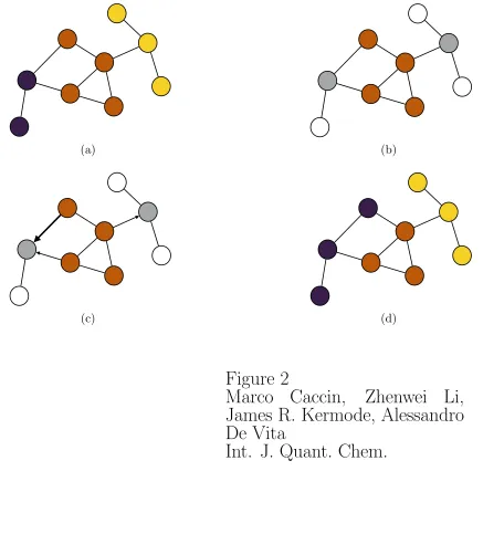
connected subgraphs at all stages. Fig. 2 illustrates a step of the digestive ripening process
for a small example graph.
QM region update
After the partitioning and on the basis of the obtained subgraphs Si(j), each core QM
sub-region is carved out of the whole system, and buffer atoms bond terminations are then added
as previously explained, to guarantee convergence of core atom forces as already discussed.
We note that isolated “outlier” clusters whose sizes are significantly higher than average can
occur at this stage, although in our experience the procedure outlined in the previous section
is sufficiently effective to drastically limit their number. These can be treated with a trivial
modification of the partitioning scheme outlined above, where the partitioning loop is run
using a slightly lower initial ˆk =k−kres target number of subdomains, keeping kres blocks
the kres largest clusters. The resulting swarm of k atomic clustersCi∪ Bi can at this point
be simultaneously sent for calculation.
As an MD simulation progresses, the QM region is automatically tracked and selected,
and only every so often is the difference between two QM regions of subsequent timesteps
(from now on designated as ‘old’ and ‘new’) sufficient to justify the execution of an ex novo
partitioning and buffering. Avoiding such operations when they are not necessary increases
the continuity of the QM clusters along the system trajectory, so that when possible we assign
the same set of atoms to the same set of processors. This is important for efficiency, since
whenever a new QM cluster is ‘similar enough’ to the old one, the wavefunctions and electron
density already present in memory can be used as the starting point for a continuation run,
which can significantly reduce the time to solution. To decide whether or not updating
the partitioning of the QM region C, similarity criteria are first applied to it as a whole:
if neither the set of atoms in C nor the list of atomic bonds in C ∪ B has changed, a new
partitioning and cluster carving procedure is avoided and the previouskQM clusters may be
reused. In this case the atomic positions of the old QM clusters are simply updated in place,
and we additionally check each new buffered cluster for compatibility with its previous state
through a checklist: (i) the set of atoms Ci∪ Bi has not changed, (ii) the lattice vectors have
not changed (only meaningful if clusters are periodic along any direction), (iii) the mean
squared displacement of atomic positions between new and old cluster is less than a given
threshold that depends on the QM engine in use. If for a given cluster all these criteria are
met, the setup already present in memory is suitable for a continuation of the previous QM
calculation.
Results: performance of the ensemble parallel scheme
In the following we present the results of tests performed on the Mira IBM Blue Gene/Q
(BG/Q) machine located at the Argonne Leadership Computing Facility. Each BG/Q
com-pute node is a PowerPC A2 1600MHz processor containing 16 cores capable of 4-way
hy-perthreading.34 We used the plane-wave DFT package VASP 5.3,6 which is parallelised via
MPI only and thus allows up to 16 processes per compute node. Electronic exchange and
The QM calculation step is by far the most computationally expensive step of any
QM/MM approach. We will thus concentrate on the performance of our novel ensemble
DFT scheme for QM/MM calculations, which is largely determined by the quality of the
multi-step partitioning algorithm we developed, and can be measured in terms of the total
computational cost and time to solution (t.t.s.) of a DFT force evaluation for a given core
QM region C contained in a larger system. The tuneable parameters of the scheme are (i)
the number of CNs assigned to each DFT instance NCN and (ii) the number k of partitions
in which to divide C. The parameters that intrinsically depend on the system under
investi-gation are (i) the total number of core atoms|C| and their geometry, and (ii) the buffer size
necessary to obtain converged QM forces for a given core QM region.
We first test the scaling properties of our DFT package of choice to identify the optimal
combination of atomic cluster size |C ∪ B|andNCN compatible with the computing
architec-ture in use. In the limit of a perfectly linear scaling DFT code and vanishing buffer region,
there would be evidently no need to split C and the best choice would be to run a single
calculation on all the available CNs; in other scenarios, however, dividing the problem is
likely to be advantageous. Based upon the computed benchmarks, we fixedNCN = 64 nodes
(equivalent to 1024 compute cores) and tune k to produce individual QM clusters with sizes
|C ∪ B| ∼ 300 atoms. According to the optimal tiling requirements previously illustrated,
we set the number of partitions to k = 2N −1 for some integer N. To investigate the weak
scaling properties of our method we choose a physical system of real interest: a
configura-tion of atoms in the neighbourhood of a crack tip in amorphous silica (a-SiO2) under tensile
load, illustrated in Fig. 3. Periodic boundary conditions (PBC) are applied along the crack
front direction (z) with periodicity 30 ˚A, providing suitable boundary conditions for the
crack slab while still reproducing well the radial distribution function of the real amorphous
(hence non-periodic) material. The regionC, shown in red in Fig. 3b, is the minimal QM core
region necessary to obtain an accurate description of bond rupture and crack propagation
in the modelled material. Due to long-range electrostatic interactions in the system, the
buffer region is significantly larger than this relatively small core region. The partitioning of
C is performed in 3 steps: (i) iterative spectral bisectioning; (ii) merging of the two smallest
and optimise the shapes of Ci.
A weak scaling benchmark needs a set of tasks of increasing problem size to which
pro-portionally increasing computing capability are allocated. In our system a useful definition
of problem size is the number of accurate DFT forces required in region C, which is equal
to the number of atoms |C|; the computing capability is the total number of CNs of the
ensemble QM/MM calculation. We can obtain different problem sizes by replicating the
system alongz and keeping the ratio|C|/k constant. The presence of surfaces in the system
makes the buffer sizes |Bi| less predictable, but with this choice the ratio between surface
and bulk atoms is kept constant. A scenario in which replication of the system along the
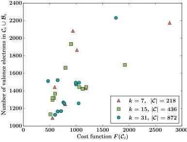
z axis is necessary is, for instance, the study of quasi-3D crack fronts. Fig. 4 shows, for a
clusterCi∪ Bi, the correlation between the cost function F(Ci), which is the variable driving
the partitioning process, and the computational cost of the DFT calculation of the cluster
Ci∪ Bi, which we can assume to be a monotonically increasing function of the number of
va-lence electrons. For the reasons already mentioned (e.g., presence of surface atoms, complex
buffering and bond termination heuristics), perfect correlation is not to be expected, but F
is nevertheless a representative quantity which is meaningful to equalise across subgraphs.
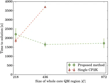
The timing results for t.t.s. for a single-point DFT calculation is shown in Fig. 5 for
the case of continuation calculations in which the in-place update of all clusters Ci ∪ Bi
has occurred. In our method the time to calculate all forces in C is the maximum t.t.s.
encountered while concurrently carrying out all the k DFT calculations on the separate
clusters. The overall good scaling of the ensemble method is easily explained once we note
that the generated clusters have about the same number of atoms, regardless of the total
problem size |C|. Moreover, moving to larger systems at the same time as increasing k
can reduce the overall t.t.s., both by producing better cluster size distributions and by the
progressively lessening effect of the presence of one computing block assigned to the classical
dynamics. The minimum size of the test system containing a complete crack front as in
Fig. 3b contains |C| = 218 atoms, which in a non-ensemble framework would result in a
single large cluster (periodic along z) of |C ∪ B| ∼1300 atoms for which a plane-wave DFT
code is no longer a viable choice. For a comparison with the current state-of-the-art codes, we
parameters. CP2K allows hybrid MPI/openMP parallelism, thus making full use of all the
available 64 threads per compute node. While the t.t.s. of the two methods are comparable
for sufficiently small system sizes, the advantage of splitting the workload across independent
executables becomes evident. It should also be noted that the overall computational cost of
carrying out a single DFT calculation would be in real terms actually almost double that
shown as red triangles in Fig. 5, due to tiling inefficiency of the kind depicted in Fig. 1a,
not incurred in the ensemble approach. Furthermore, our ensemble framework is not tied to
a specific DFT code: it can be then envisioned that choosing the best performing code for
a given machine architecture would lower the t.t.s. of each parallel calculation while at the
same time keeping the scaling trend intact.
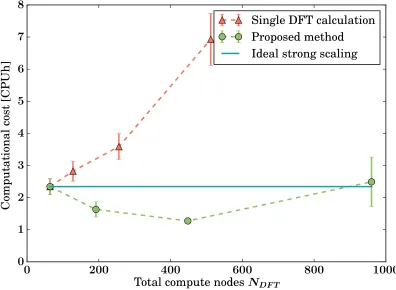
We next analyse the strong scaling of our method, i.e. the speedup when tackling a fixed
size problem with increasing computing resources. A minimal realistic crack front in a-SiO2
is too large a system to be investigated by a single plane-wave DFT calculation, so for these
tests we instead studied a crack front in crystalline Si comprising|C| = 111 core QM atoms.
Moreover, the covalent nature of the bonding leads to shorter-range interactions, so the
buffer regions required are much smaller.19 As can be observed in Fig. 6, a single plane-wave
DFT code cannot efficiently make use of the increasingly available computational power;
conversely, excellent strong scaling can be obtained when the task is split among several
independent instances of the same DFT executable. By means of this test, for the given
system and DFT engine we can set the variable k so that the overall computational cost is
minimised (here obtained for k = 7).
MACHINE LEARNING MOLECULAR DYNAMICS
We next briefly review a ML MD scheme targeted at efficiently harnessing the stream of QM
data flowing from CPU-intensive first principles calculations like those described above. A
way to combine the ensemble parallelism approach with this scheme, with the potential of
significantly enhancing the usefulness of both techniques in large scale simulations, will be
discussed in the Outlook section below. Rather than attempting to build up a full picture
networks8 or Gaussian Process (GP) regression,9 our approach focusses on learning the QM force acting on an atom given its local environment. We use GP regression35 to infer
the most probable QM force on a new atomic environment given a database of previous
observations and a Gaussian prior distribution expressed via a smooth covariance kernel.
Direct force learning circumvents the numerical errors associated with the differentiation of
a PES constructed on the ML teaching set points for the evaluation of forces in
energy-based ML schemes. Moreover, a force-learning scheme enables us to add novel information
to the teaching database ‘on-the-fly’, with the QM engine being called only if the information
within the existing database is insufficient to infer QM forces on a configuration of interest.
In this way, the force accuracy can be kept closely in line with that of the QM target.
For simple test systems we find that the training data becomes essentially complete after a
limited initial training period, after which the predicted ML forces are sufficient to accurately
determine the further trajectory evolution. For more complex systems the rate at which new
data needs to be learnt systematically decreases as the phase space of the system already
explored increases, and intensive learning only takes place where novel chemical complexity
is encountered. As a further appealing feature of ML methods, large-scale teaching datasets
can be generated by combining data from any compatible set of calculations, and results
from separate simulations across different projects can be integrated in one progressively
growing knowledge pool.
Learning Forces From Atomic Environments
Given an atom, its local atomic environment is defined as the set of neighbouring atoms
within a prescribed cutoff radius. For covalent materials, such as Si, considering only the
∼100 neighbouring atoms within 8 ˚A is sufficient to converge DFT forces to an accuracy of
0.05 eV/˚A, which is comparable with the typical accuracy of forces in a DFT calculation.
For systems where long range electrostatic forces are important, such as oxides, we envisage
that a global classical Coulomb model based on fixed multipole moments could be added to
the ML-predicted short-ranged forces to produce a faithful model of the overall interactions.
Developing a representation for atomic environments that is appropriate for learning QM
regression problem, the representation should possess the intrinsic symmetries of the force,
and thus be invariant under rigid rotation, translation, inversion as well as any permutation
of atoms of the same chemical species. As a first approach, we have proposed a simple vector
description of the local environment around an atom consisting of a set{Vi} ofnIV internal
vectors (IVs) which, by construction, encode the relevant symmetries of the QM force vector.
A set of IVs can be defined using the formula
Vi = Nneighb
X
q=1
ˆrq exp
" −
rq
rcut(i)
p(i)#
. (6)
This set can be augmented by additional vectors such as forces derived from relevant simpler
interaction models, e.g., the Stillinger-Weber interatomic potential36 in the case of Si or
the Tangney-Scandolo linear scaling polarisable interatomic potential in the case of a-SiO2
system.37 Testing reveals that such augmentation can significantly improve force prediction
accuracy, suggesting that simpler force fields — while not necessarily accurate enough to be
used on a standalone basis — encode useful information which can be exploited by learning
the correlation of the forces they predict with the target QM forces.
To parametrise the method for a new material, an initial dataset of relevant configurations
(atomic positions and corresponding forces) is required. An appropriate set of IVs such as
those in Eq. 6 must then be chosen, typically as the minimal set of vectors that carry good
correlation with the target forces, i.e., lead to a low cross-validation error over the database.
We envision that this process of optimal features selection could be automated with widely
used techniques such as the LASSO method38outlined in Ref. 39. The input space descriptor
used in our scheme is a ‘feature matrix’ X ∈ RnIV×nIV constructed from the projection of
all IVs onto the inner basis set {Vˆi = Vi/|Vi|}. This representation is used in a Gaussian
kernel function
k(Xi,Xj) = exp −d(Xi,Xj)2/2σcov2
, (7)
to construct the GP covariance matrixC will have entries
Cij =k(Xi,Xj) +σ2errδij, (8)
whered(Xi,Xj) is an appropriately preconditioned Euclidean distance between teaching set
pre-liminary cross-validation procedure over a sample dataset, whileσerr represents the nominal
confidence interval of the calculated QM forces, here set to 0.05 eV/˚A. The GP regression
scheme operates in the internal vector space, so all forces are represented onto the
over-complete {Vˆi} basis set. For a configurationt, the posterior mean and variance of the force
(yt and σyt, respectively) is calculated via the standard equations
yt=kTC−1y, σy2t =κ−k
TC−1k (9)
wherek is the vector of kernel distances oft with respect to all other teaching set entries, κ
is the covariance of the test configuration with itself and y is the vector of training output
data. Finally, to reconstruct a predicted force in Cartesian space an overdetermined linear
system is solved via least squares solution.10
We note in passing that the representation used here can be naturally extended to
multi-component systems by constructing IVs only between atoms with the same chemical species,
and combining these to form an extended feature matrix with a block structure that reflects
the presence of the different species. Preliminary results indicate that this approach ensures
that ML force prediction remains accurate for SiO2 and SiC systems using similar, if slightly
larger, database sizes (for full details cf. Ref. 10, Supplementary Material). Furthermore, our
approach is also straightforwardly applicable to learn from higher-level quantum chemistry
approaches. Namely, forces obtained from higher level schemes can be fed to the database in
exactly the same way as DFT ones. An interesting scenario would arise in systems for which
DFT and higher level (e.g., Quantum Monte Carlo, coupled cluster, etc.) forces were to be
found substantially equivalent in many configuration space regions (e.g., close to structural
minima corresponding to stable or metastable phases), but significantly different only in
specific circumstances (e.g., for level-crossing configurations in molecular systems). If the
relevant ‘discrepancy’ phase space regions were reasonably precisely identified in some
well-controlled example system, a hybrid ML database could be constructed and grown in our
scheme by computing the relatively affordable DFT forces where these are correct, and the
expensive higher level forces only when needed: that is, just for the configurations where
these are expected to differ significantly from the DFT ones. We speculate that such an
of the works by Refs. 40, 41.
Validation of the Force Learning Scheme
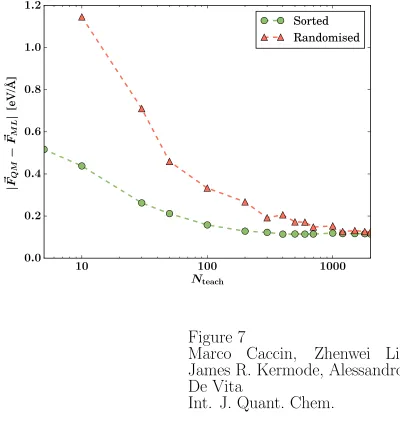
Systematic validation of our ML force calculation scheme has been carried out for crystalline
and molten silicon model systems.10 We find that converged prediction accuracy is typically
achievable using only a few hundred most relevant data points selected from the full database.
This is illustrated by Fig. 7, which includes a comparison with the predictions obtained
using a teaching database chosen randomly from a large database. Clearly, searching for and
selecting the most relevant data configurations for each new test configuration is preferable,
and is thus used throughout the scheme. By using a fixed-size ‘closer configurations’ subsets
also ensures that the overall computational cost of ML-predicting the force on an atom
(of the order of 10−1 CPU-seconds in our tests) scales linearly with the database size. To
appreciate the efficiency gain associated with the ML method, calculating the same force ex
novo with a first principles method would typically require at least ∼102 CPU-seconds.
To perform the ML on-the-fly, we combine the predicted ML forces with the LOTF
predictor-corrector algorithm. We adjust the length of the predictor-corrector cycle, and
hence the required frequency of QM calculations, in response to the force errors measured
at each corrector stage. Our results for Si suggest that using ML allows the extrapolation
length to be increased by at least a factor of three compared to the previous approach based
on fitting to a fixed functional form at each QM force evaluation step.5,10 Along an MD
trajectory, we find that concentrated QM training is necessary at times when more chemical
novelty is encountered, while fewer or no further QM calculations are needed if the system
visits configuration space regions that have already been visited, and to the extent that they
have effectively been learned. For relatively simple systems, such as low temperature ones,
a sufficiently complete database can be obtained after a limited initial period of training,
after which further QM calculation are just very occasionally needed to predict forces in the
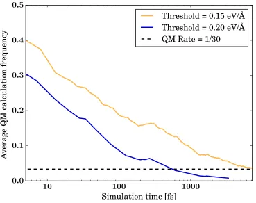
accessible portions of phase space. Fig. 8 shows results from simulations performed on Si at
1000 K using density functional tight binding42forces as the QM target. This calculation was
carried out by monitoring the real error associated with the ML-predicted forces, compared
error thresholds were selected to decide when to add additional QM information to the
database. For the larger error threshold, QM training only happens during the first 2 ps
and no further QM calls are needed, while at a tighter accuracy threshold occasional QM
calls are still necessary after 7 ps. A stable predictor-corrector cycle length of 30 fs (i.e.
a QM call frequency of 1/30 using a standard 1 fs time step for the dynamics) can be
reached after 7 ps of simulations, demonstrating the capability of the new approach to
accelerate first principles MD simulations. We note that monitoring predictor-stage actual
force errors is a safe criterion, since this lifts the need for error estimations. Moreover, the MD
trajectory is eventually integrated via ML-forces generated along the corrector stride, which
by construction connects two system configurations well represented by the ML database, so
that the ML force errors are significantly reduced.
OUTLOOK
In this work we have addressed two recent technical developments aimed at enabling efficient
force-based QM/MM simulations on large HPC resources. First, we presented an ensemble
parallelisation approach to split large individual QM calculations into several manageable
portions. We then outlined a novel machine learning scheme that strives to predict, rather
than recalculate, QM forces when encountering atomic configurations similar to those
previ-ously seen. In this section we discuss some implications of these two techniques, and suggest
ways in which they could be combined to improve the information efficiency of
simulat-ing large atomistic systems. In our previous discussion of the ensemble parallelism scheme,
the compute node allocation was filled by setting the total number k of QM subregions
to k = 2N −1. This assumes that HPC partitions composed of 2N blocks are allocatable
through the queueing system, so k is chosen to keep one block free for non-QM work.
How-ever, once the constraint of running the same tasks on all blocks is removed, the flexibility
of our partitioning scheme could be exploited more comprehensively. Namely, it would be
straightforward to choose a smaller k value for the QM zone partitioning and fill up the
additional freen= 2N−1−kcompute node blocks withany other tasks consistent with
clusters of significantly larger than average dimensions after the partitioning and buffering
phases). In particular, more QM cluster calculations could be performed to provide
addi-tional QM information where needed. As anticipated in the introduction, an unavoidable
consequence of simulating large QM zones of a priori unpredictable chemical behaviour is
that ‘new’ chemical events could occur in any set of localised QM subregions during the
dynamical evolution of the system. In any such region the ML-predicted forces are by
defini-tion less reliable and the local frequency of necessary QM calculadefini-tions must correspondently
grow. An accuracy increase could be easily achieved by shortening the general
predictor-corrector stride of the LOTF scheme. This would be inefficient, as QM calculations would
then time-densify throughout the QM zone, even where this was not needed.
A much better strategy would consist of augmenting the ML database intake rate limited
to the more ‘difficult’ QM subregions, where asynchronous supplementary QM calculations
would be carried out. This way, any critical subregion experiencing a higher rate of chemical
novelty would be allocated QM computations occurring at a commensurately higher rate.
Such ‘preconditioning’ of the ML database growth rate over the QM zone would in turn allow
using a unique, optimally large predictor-corrector stride throughout the system, while fresh
QM information would be effectively computed in a fully importance-sampled way, in both
the space and time domains. In a simple implementation, carrying out extra calculations at
half the extrapolation length for a set of the n most critical QM subregions would provide
new QM information for these at twice the normal frequency without compromising the
load-balancing characteristics of the algorithm. A simple heuristic to identify the critical
subregions would be to choose those for which the predictor force errors measured at the most
recent QM force calculation are larger. The results of the additional half length predictor
QM calculations would just be added to the ML database, to improve the accuracy of the
following corrector stage and any ML-inferred forces from this point on.
To summarise, the procedure outlined above would combine ML force prediction with
the ability of carrying out QM calculations on small selected system QM zone subregions.
In particular, QM zone partitioning would make it possible to lift the predictor-corrector
algorithm standard constraint of carrying out accurate calculations at the same fixed times
inter-polation properties of the corrector loop, thus leaving unaffected the robustness of the LOTF
scheme (the general idea is, however, implementation independent, as any learning QM/MM
scheme could consider using partitioning to minimise QM calculations). We speculate that
in many situations this would enable a significantly more efficient usage of the available HPC
resources.
We finally note that carrying out additional QM calculations as suggested here would be
expected to decrease, rather than increase, the overall ML database growth rate per unit
simulated system time, compared with the synchronous scheme of Ref. 10 used with a shorter
predictor-corrector stride. However, in either running modality the databases associated with
ML methods are expected to grow large very quickly during the system evolution, and could
be very large from start when incorporating QM data from previous simulations for similar
systems. For this reason, we envisage that specific (‘big data’) techniques will eventually be
needed to effectively deal with databases containing millions of configurations. For instance,
a hierarchical clustering approach could be used to build a ‘social network’ encapsulating
the dendrographic relationship between teaching data to identify the principal nodes of the
network of configurations.
ACKNOWLEDGEMENTS
This work was funded by the Engineering and Physical Sciences Research Council under grant
numbers EP/L014742/1 and EP/L027682/1. Additional financial support was provided by
Argonne National Laboratory through a collaboration with the Thomas Young Centre and
by the Rio Tinto Centre for Advanced Mineral Recovery based at Imperial College London.
An award of computer time was provided by the Innovative and Novel Computational Impact
on Theory and Experiment (INCITE) program. This research used resources of the Argonne
Leadership Computing Facility, which is a DOE Office of Science User Facility supported
References
1. J. R. Kermode, G. Peralta, Z. Li, and A. De Vita, Procedia Materials Science 3, 1681
(2014).
2. M. Ciccotti, J. Phys. D Appl. Phys. 42, 214006 (2009).
3. J. R. Kermode, T. Albaret, D. Sherman, N. Bernstein, P. Gumbsch, M. C. Payne,
G. Cs´anyi, and A. D. Vita, Nature 455, 1224 (2008).
4. J. Song and W. Curtin, Nat. Mater. 12, 145 (2013).
5. N. Bernstein, J. R. Kermode, and G. Cs´anyi, Rep. Prog. Phys. 72, 026501 (2009).
6. G. Kresse and J. Hafner, Phys. Rev. B 47, 558 (1993).
7. S. J. Clark, M. D. Segall, C. J. Pickard, P. J. Hasnip, M. I. J. Probert, K. Refson, and
M. C. Payne, Zeitschrift f¨ur Kristallographie 220 (2005).
8. J. Behler and M. Parrinello, Phys. Rev. Lett. 98, 146401 (2007).
9. A. P. Bart´ok, M. C. Payne, R. Kondor, and G. Cs´anyi, Phys. Rev. Lett. 104 (2010).
10. Z. Li, J. R. Kermode, and A. De Vita, Phys. Rev. Lett. 114, 096405 (2015).
11. V. Botu and R. Ramprasad, Int. J. Quantum Chem. (2014).
12. C.-K. Skylaris, P. D. Haynes, A. A. Mostofi, and M. C. Payne, J. Chem. Phys. 122,
084119 (2005).
13. J. M. Soler, E. Artacho, J. D. Gale, A. Garc´ıa, J. Junquera, P. Ordej´on, and D. S´
anchez-Portal, J. Phys.-Condens. Mat. 14, 2745 (2002).
14. G. Cs´anyi, T. Albaret, M. Payne, and A. De Vita, Phys. Rev. Lett. 93, 175503 (2004).
15. G. Cs´anyi, G. Moras, J. R. Kermode, M. C. Payne, A. Mainwood, and A. D. Vita, in
16. G. Cs´anyi, S. Winfield, J. R. Kermode, A. De Vita, A. Comisso, N.
Bern-stein, and M. C. Payne, Expressive programming for computational physics in
fortran 95+ (2007), URL https://camtools.cam.ac.uk/access/content/group/
5b59f819-0806-4a4d-0046-bcad6b9ac70f/IoP_libatoms.pdf.
17. J. VandeVondele, M. Krack, F. Mohamed, M. Parrinello, T. Chassaing, and J. Hutter,
Comput. Phys. Commun. 167, 103 (2005).
18. W. Kohn, Phys. Rev. Lett. 76, 3168 (1996).
19. A. Peguiron, L. Colombi Ciacchi, A. De Vita, J. Kermode, and G. Moras, J. Chem.
Phys. 142, 064116 (2015).
20. J. Kermode, L. Ben-Bashat, F. Atrash, J. Cilliers, D. Sherman, and A. D. Vita, Nat.
Comms. 4 (2013).
21. G. Moras, L. C. Ciacchi, C. Els¨asser, P. Gumbsch, and A. De Vita, Phys. Rev. Lett.
105, 075502 (2010).
22. A. Gleizer, G. Peralta, J. R. Kermode, A. De Vita, and D. Sherman, Phys. Rev. Lett.
112, 115501 (2014).
23. J. R. Kermode and M. Caccin, libAtoms/gepsipy package.
24. B. Kernighan and S. Lin, Bell Syst. Tech. J. (1970).
25. C. Fiduccia and R. Mattheyses, Des. Autom. 1982. 19th Conference on. IEEE pp. 175–
181 (1982).
26. D. Spielmat, inProc. 37th Conf. Found. Comput. Sci.(IEEE Comput. Soc. Press, 1996),
pp. 96–105.
27. A. Pothen, H. D. Simon, and K.-P. Liou, SIAM J. Matrix Anal. Appl. 11, 430 (1990).
28. G. Karypis and V. Kumar, SIAM J. Sci. Comput. 20, 359 (1998).
29. A. A. Hagberg, D. A. Schult, and P. J. Swart, inProceedings of the 7th Python in Science
30. J. E. Gentle, L. Kaufman, and P. J. Rousseuw, Biometrics47, 788 (1991).
31. M. Fiedler, Czechoslov. Math. J. 23 (1973).
32. M. Fiedler, Czechoslov. Math. J. 25 (1975).
33. D. Lee, S. Park, J. Lee, and N. Hwang, Acta Mater. 55, 5281 (2007).
34. R. A. Haring, M. Ohmacht, T. W. Fox, M. K. Gschwind, D. L. Satterfield, K. Sugavanam,
P. W. Coteus, P. Heidelberger, M. A. Blumrich, R. W. Wisniewski, et al., Micro, IEEE
32, 48 (2012).
35. D. MacKay, Information theory, inference and learning algorithms (Cambridge Univ
Press, Cambridge, 2003).
36. F. H. Stillinger and T. A. Weber, Phys. Rev. B 31, 5262 (1985).
37. J. R. Kermode, S. Cereda, P. Tangney, and A. De Vita, J. Chem. Phys. 133, 094102
(2010).
38. R. Tibshirani, J. R. Stat. Soc. Ser. B Stat. Methodol. pp. 267–288 (1996).
39. L. M. Ghiringhelli, J. Vybiral, S. V. Levchenko, C. Draxl, and M. Scheffler, Phys. Rev.
Lett. 114, 105503 (2015).
40. J. Grossman and L. Mitas, Phys. Rev. Lett. 94, 056403 (2005).
41. A. P. Bart´ok, M. J. Gillan, F. R. Manby, and G. Cs´anyi, Phys. Rev. B88, 054104 (2013).
42. M. Elstner, D. Porezag, G. Jungnickel, J. Elsner, M. Haugk, T. Frauenheim, S. Suhai,
Figure 1: Tiling options for running a QM/MM calculation on a 16-block job partition:
each small square corresponds to one block, and an executable can only run on 2N blocks.
(a) The allocation is only partially occupied; (b) The allocation fully occupied, but the MD
partition is unnecessarily large; (c) Optimal partition tiling enabled by the ensemble parallel
QM calculations proposed in this work.
Figure 2: Example step of the digestive ripening algorithm on a connected graph comprising
k = 3 subgraphs: (a) Initial partitioning; (b) Identification of the region i∗ most dissimilar
from the others (brown vertices/atoms) and its neighbour vertices (in grey); (c) Calculation of
gain for all possible moves (three arrows) and selection of the highest gain move (bold arrow);
(d) Updated partitioning, where the k subgraphs are more commensurate and compact.
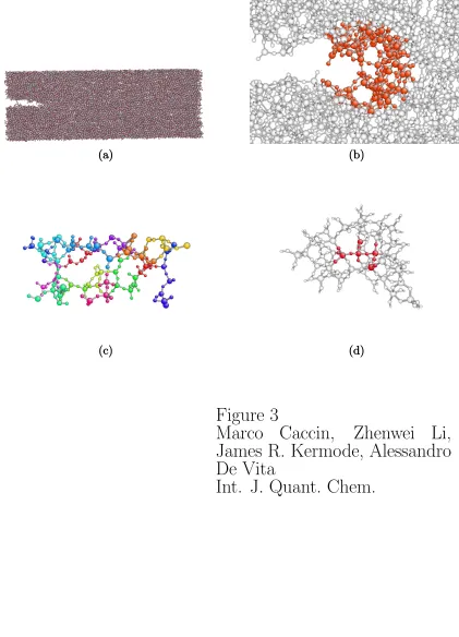
Figure 3: Benchmark system for weak scaling: crack tip of a-SiO2. (a) Minimal size whole
system for QM/MM simulation of SiO2 glass fracture, comprising ∼30000 atoms. (b) Crack
tip closeup. The core QM region C is represented in red. Larger beads are Si atoms, smaller
beads are O atoms. Here|C|= 218 atoms. (c)C partitioned ink = 15 parts: each connected
set of equally coloured atoms corresponds to a different Ci (PBCs apply). |Ci|= 15 atoms on
average. (d) Example of a cluster Ci∪ Bi sent for DFT calculation. C atoms are represented
in red, buffer atoms are white. The cluster contains |Ci∪ Bi| ∼250 atoms.
Figure 4: Correlation between cost function of each as-partitioned core QM subregion Ci
and the number of valence electrons of core and buffer region of the atomic cluster used to
calculate forces inCi. The system is the a-SiO2crack tip used for the weak scaling benchmark
(cf. Fig. 3). Results are shown for 3 systems comprising a different number of total core
Figure 5: Weak scaling of the ensemble parallel method: the time to solution is given as
a function of the problem size, here the number |C| of atoms in the full core QM region.
For the ensemble method (green circles), the ratio between the number of core QM atoms
and the number of compute nodes (CNs) for the total calculation is kept approximately
fixed: problem sizes of |C| = 218,436,872 atoms correspond to splitting the full QM region
in k = 7,15,31 parts, respectively. The total CNs assigned to the DFT calculations are
given by NDFT = 64·k, corresponding to a concurrent use of 448, 960, and 1984 CNs. The
cost of a single CP2K calculation for the 218 and 436 atom systems using NDFT = 512 and
1024 nodes, respectively, is shown for comparison (orange triangles). Ideal scaling would
correspond to a constant time to solution.
Figure 6: Strong scaling of ensemble parallel method: the total computational cost —
measured as the wall-clock time taken by the calculation times the total number NDF T of
compute nodes used — is shown as a function of the total number of compute nodes assigned
to DFT calculations NDFT. The core QM region (here, a Si crack tip) is kept constant, and
the ensemble results (green circles) are shown for partitionings into k = 1,3,7,15 parts
respectively, corresponding to a concurrent use of NDFT = 64·k compute nodes. For a
comparison with a single DFT calculation on the whole QM zone using the same DFT code,
the results are shown for NDFT = 64, 256, and 512 compute nodes (orange triangles). Ideal
scaling would correspond to constant computational cost (blue solid line).
Figure 7: Accuracy of ML force predictions for bulk Si at 1000 K as a function of the
teaching database size. The teaching set of size Nteach is extracted from a larger database
either randomly (orange triangles) or by selecting the configurations nearest to the one
for which force prediction in needed (green circles). Convergence is more rapidly achieved
when the most relevant data are selected, and in both cases the force error converges to an
Figure 8: Running average rate of fresh QM force calculations necessary to guarantee that
errors of the ML force prediction do not exceed a given threshold, here set to 0.15 eV/˚A
(yellow) and 0.2 eV/˚A (blue). The dashed horizontal line represents the QM rate in the case
Figure 1
Marco Caccin,
Zhenwei Li,
James R. Kermode, Alessandro
De Vita
Figure 2
Marco Caccin,
Zhenwei Li,
James R. Kermode, Alessandro
De Vita
Figure 3
Marco Caccin,
Zhenwei Li,
James R. Kermode, Alessandro
De Vita
0 500 1000 1500 2000 2500 3000 Cost functionF(Ci)
1000 1200 1400 1600 1800 2000 2200 2400
N
um
be
r
of
va
le
nc
e
el
ec
tr
on
s
in
Ci
∪
Bi
[image:31.612.100.485.98.390.2]k = 7, |C|= 218 k= 15, |C|= 436 k= 31, |C|= 872
Figure 4
Marco Caccin,
Zhenwei Li,
James R. Kermode, Alessandro
De Vita
218 436 872 Size of whole core QM region|C|
0 500 1000 1500 2000 2500 3000 3500 4000
T
im
e
to
so
lu
ti
on
[s
]
[image:32.612.102.479.99.386.2]Proposed method Single CP2K
Figure 5
Marco Caccin,
Zhenwei Li,
James R. Kermode, Alessandro
De Vita
0 200 400 600 800 1000 Total compute nodesNDF T
0 1 2 3 4 5 6 7 8
C
om
pu
ta
ti
on
al
co
st
[C
P
U
h]
[image:33.612.105.501.86.376.2]Single DFT calculation Proposed method Ideal strong scaling
Figure 6
Marco Caccin,
Zhenwei Li,
James R. Kermode, Alessandro
De Vita
10 100 1000
Nteach
0.0 0.2 0.4 0.6 0.8 1.0 1.2
|
~ FQ
M
−
~ FM
L
|
[e
V
/˚A
]
[image:34.612.104.504.99.531.2]Sorted Randomised
Figure 7
Marco Caccin,
Zhenwei Li,
James R. Kermode, Alessandro
De Vita
10 100 1000 Simulation time [fs] 0.0
0.1 0.2 0.3 0.4 0.5
A
ve
ra
ge
Q
M
ca
lc
ul
at
io
n
fr
eq
ue
nc
y
[image:35.612.111.480.97.389.2]Threshold = 0.15 eV/ ˚A Threshold = 0.20 eV/ ˚A QM Rate = 1/30