nuclear science and technology
APPLICATION OF THE METHODS OF
STATISTICAL ANALYSIS OF PSEUDO-RANDOM
SIGNALS TO THE INTERPRETATION
OF FIELDS TRIALS ON THE ATMOSPHERIC
TRANSPORT OF ACTIVE PRODUCTS AND
TO ESTIMATE OF CONFIDENCE LIMITS
m
Report
EUR 9536 EN
nuclear science and technology
APPLICATION OF THE METHODS OF
STATISTICAL ANALYSIS OF PSEUDO-RANDOM
SIGNALS TO THE INTERPRETATION
OF FIELDS TRIALS ON THE ATMOSPHERIC
TRANSPORT OF ACTIVE PRODUCTS AND
TO ESTIMATE OF CONFIDENCE LIMITS
D. OLIVARI
von Karman Institute for Fluid Dynamics Environmental and Applied Fluid
Dynamics Department Chaussée de Waterloo, 72 B-1640 Rhode Saint Genèse - Belgium
Contract No. ECI 927-B7221-82-B
FINAL REPORT
Directorate-General for Science, Research and Development
Information Market and Innovation Bâtiment Jean Monnet
LUXEMBOURG
LEGAL NOTICE
Neither the Commission of the European Communities nor any person acting on behalf of the Commission is responsible for the use which might be made of the following
information
TABLE OF CONTENTS
ABSTRACT i
1. INTRODUCTION 1
2. SOME EXPERIMENTAL OBSERVATIONS 3
3. MODELS FOR DISPERSIONS OF PASSIVE CONTAMINANTS 7
IN TURBULENT FIELDS 7 3.1 Notes on terminology 8
3.2 The gradient diffusion equations 11
3.3 The statistical approach 14 3.4 The random walk approach 17 3.5 The effect of molecular diffusivity 21
4. STATISTICAL PROPERTIES OF THE CONCENTRATION . . . . 23
4.1 The probability density function 23 4.2 Some practical problems related to p.d.f. . . . 24
5. EFFECTS OF MEASUREMENT INSTRUMENTS 29
5.1 The sensor effects 29 5.2 Analysis of results 38
6. INTERMITTENCY AND p.d.f 51 6.1 Definition of intermittency 52
6.2 The combination of intermittency and
concentration 55
7. EFFECT OF EXTERNAL RANDOM CONDITION 68
8. CONCLUSION 72
ECI 927-B7221-82-B
An attempt is made at identifying the most important factors which introduce difficulties in the analysis of results from tests on pollutant dispersal : the unsteadiness of the phenomenon, the effect of external uncontrollable parameters, and the inherent complexity of the problem itself.
The basic models for prediction of dispersion of passive contaminants are discussed, and in particular a Lagrangian approach which seems to provide accurate results.
For the analysis of results many problems arise. First the need of
computing for the results the statistical quantities which describe them: the mean, the variance and higher order moments are important.
It is shown that there is no easy solution if the duration and/or the
number of independent "events" to be analyzed are too limited. The probability density function provides the most useful information, but is not easy
to measure. A family of functions is recalled which predict reasonably well the trend of the pdf. Then the role of intermittency is shown in some detail. Its importance cannot be underestimated and its relationship to pdf and the effects on measurements are shown to be rather complex.
1. INTRODUCTION
The purpose of the present research is to determine the limits of confidence which can be associated with concentra-tion measurements in full scale tests, where most of the
domi-nant elements governing the phenomenon are not under full c o n t r o l .
These may be an incomplete knowledge of the m e t e o r o l o -gical conditions, the uncertainties of the characteristics of
the release source, and even accuracies of the measuring instruments
Knowing that the problem of turbulent diffusion is one of the most complex in fluid dynamics, adding all the u n c e r t a i n t i e s associated with experiments in real atmospheric flows, makes the task very daunting. Really, one should start from the analysis of the solution of Navier-Stokes and diffusion equations for stochastic boundary c o n d i t i o n s .
For the present research, the author hopes to arrive at some useful conclusions of practical interest, but so far as the work advances the problem becomes so wide and takes on so many facets that a sort of unitary view of the problem still seems difficult to achieve.
The present report is not intended to provide any con-clusion, but just illustrates some of the subjects available in the literature and which have attracted the interest Of the author as useful in the present context. Of course some discussion will be made and some conclusions drawn, but the author himself is not fully satisfied nor absolutely sure that they should not be re-vised in future research.
d i s p e r s i o n p h e n o m e n a .
The second approach is based on the analysis of the fundamental equation governing the dispersion phenomena in tur-bulent flow f i e l d s . The hope here is to be able to understand and m a s t e r the essential elements involved without running into the problem of too big mathematical difficulties in the solution. That the problem in general is not so easy has already been said and the sort of d i f f i c u l t i e s which may be encountered when trying to deal with the whole situation is clearly illustrated in the a n a l y s i s of F a r m e r . N e v e r t h e l e s s , if one really wants to arrive at c o n c l u s i o n s supported by an understanding of the phenomena in-v o l in-v e d , this is the only way to approach the problem.
Again there are two possibilities of looking at it; one which may be called m i c r o s c o p i c and the other m a c r o s c o p i c . W i t h o u t going into too much d e t a i l , one can establish the dif-ference between the two by considering that in the first one
the real m e c h a n i s m of turbulent dispersion is analyzed and the final results obtained by the logical consequences of each step. In the second only the gross features are looked at, such as mean c o n c e n t r a t i o n , m e a n d e r i n g , intermittency and so o n , the finest details being hidden or covered by more or less local c o e f f i c i e n t of d i f f u s i o n of universal nature and acting at a scale much smaller than the one of interest.
The problem of the accuracy or better of the statisti-cal relevance of the measured results is also important; espe-cially if one has to take into account the averaging effect of the finite size of the instruments themselves and of the region of the flow over which they respond.
This type of approach, based on the fitting of
experi-mental data with empirical correlation is widely used and well
documented in the literature. As mentioned before, such work
is far from being as trivial as it seems from the above
state-ment, because if consistent results are looked for, they should
be based not only on sound experimental evidence, but also on a
correct interpretation of the fundamental mechanism of turbulent
dispersion. Experimental data can here be considered as
origi-nating either from full scale or wind tunnel simulated tests,
although the main field of application of such an analysis is
for the interpretation of full scale results. Accounts,
des-criptions and justification of such approaches are given by
Csanady, Larsen, Cats and Haltslag, Nieuwstad, Tsukatani,
to quote some examples.
In each case the problem is that of determining the
dependence of air pollution frequency distribution on
meteoro-logical data. The starting point can probably be traced back
to Larsen who suggested in 1969 that air pollution frequencies
in complex source areas are approximately described by a
log-normal distribution of the probability.
There are some good reasons to suggest such a
conclu-sion, and in particular the fact that this can be considered as
the limit to be achieved when dealing with large sequences of
measured air pollution concentration. In fact, it probably
can be considered as a limit situation which is reached when
it is assumed that air pollution concentrations are independent
and identically distributed.
Long s e q u e n c e s of o b s e r v a t i o n are required because air p o l l u t i o n c o n c e n t r a t i o n depends on the random fluctuation of w e a t h e r and also on the variability of emission from the source i t s e l f .
Also the actual c o n c e n t r a t i o n depends very much on the local t o p o g r a p h y near the source emission and near the m o n i t o r i n g p o i n t .
But probably the wind velocity and direction (and their v a r i a b i l i t i e s ) are the main meteorological factors d e t e r m i n i n g local c o n c e n t r a t i o n s . It should also be stated that a c t u a l , local c o n c e n t r a t i o n in itself is not a useful para-meter being a random v a r i a b l e , and so likely to be described only by a large set of i n f o r m a t i o n . Depending on the type of p o l l u t a n t and on its possible e f f e c t , what is more useful is to be able to d e s c r i b e , or predict, the statistical properties of say maximum v a l u e s , or of exceeding prescribed values for a specified time or to be within certain prescribed limits.
It is in this context that the availability of air p o l l u t i o n f r e q u e n c y distribution model is helpful because it allows the f u r t h e r e s t i m a t i o n of the required q u a n t i t i e s . It is also important here to note that there are a few different s i t u a t i o n s which may require different a n a l y s i s . Without going into the details it can be expected that different approaches should be used, let us say, for the case of distributed sources as opposed to point s o u r c e s , for the case of the data being the results of a number of individual short time releases
opposed to c o n t i n u o u s sources and so on.
More important (as will be discussed later on because it involves the a p p l i c a b i l i t y of the models t h e m s e l v e s ) is the d i f f e r e n c e between sources near the ground and elevated o n e s .
which clearly best approach the limit condition consisting of dealing with a large number of independent realisations.
For the same reason it seems that such an analysis is least well suited for the prediction of a "one-off"
release of pollutants of short duration.
Even in the best conditions there is strong evidence (see above r e f e r e n c e s ) , that the log normal distribution does not always fit the data in the best possible way (it should be stated again that the problem here is not to determine the centerline trajectory of pollutant release nor its mean concen-tration. These definitely are important parameters, even more so because the mechanism of turbulent transport is the same whether one looks for the instantaneous values or the mean one, and after all the mean concentration is nothing else than the cumulative probability of the instantaneous realisation. The relations one is looking for are, as stated before, those
giving the probabilities of having certain specified values for a specified d u r a t i o n ) .
Most of the results show some kind of variation with respect to the log normal m o d e l . Such discrepancies are not always large and it is always difficult to attribute them to a true behaviour, to the fact that the available data are in-sufficient for a correct statistical a n a l y s i s , or that (as is often said) eventual background levels are difficult to sepa-rate from the rest. The fact that these differences are often small is not sufficient to say that they can be neglected. If this can be done is some c a s e s , when the conditions are criti-cal, either because of the nature of the pollutant or because of the site, further refinement is required.
3. MODELS FOR DISPERSIONS OF PASSIVE CONTAMINANTS
IN TURBULENT FIELDS
Reviews of models for pollutant dispersal in
turbu-lent flows abound. References describing the problem are in
Hama, Csanady, Robins, Farmer, not to mention the fundamental
book of Monin and Yaglom, and the extremely interesting even
if very complex paper by Lin. In view of this there is no
point in remaking in full such a review here except to
mention a few points which are considered of primary concern.
For the sake of simplicity, all the following analyses
and examples will be made considering a time dependent,
uni-dimensional or plane flow field. Extension to multi uni-dimensional
problem and to sheared flows is discussed in the literature,
(but it is not evident that the word easily can be used for such
an extens i o n ) .
From a practical standpoint contaminants can be classified as :
- Passive
- no action on the flow field;
- uniform density, no gravity forces;
- no momentum excess or defect;
- in practice simply a tagged or marked particle.
- Active
- action on flow field;
- density difference, gravity forces;
- etc.
- Reactive
- chemical reaction, change in volume, etc.
It was said that some definition of terms to be used
to describe the turbulent transport contaminants is required.
It is in particular important to make a clear difference
between the meaning of terms such as "diffusion" and "dispersion"
DISPERSION is a general term and in most contexts it
can be used to describe all the phenomena associated with
turbulent transport.
DIFFUSION is a much more restrictive phenomenon and
when associated with turbulence it should be used with care.
It is important to note in this context that all molecular
transport phenomena can be considered as "diffusive" from a
macroscopic standpoint. This is true when the Knudsen number
is large enough, which is the case for all practical problems
of interest in our context. It was already said that for a
turbulent flow the situation is more complicated because one
is always dealing with scales which cannot be neglected in
comparison to mean flow scales. Dispersion can be considered
as diffusion only if it can be assumed to take place in a
system which has no memory of its past history. This means
that the future state of each particle in the system is only
determined by the present status of the system, independently
from the way taken to arrive at it.
As a consequence it may be stated that any variable
in a system which satisfies the above conditions must have a
correlation scale small enough in comparison to the time
in-volved in the computations. In a discretized system the
variable W. must be uncorrelated for successive time steps,
that is, its correlation is defined by Dirac delta function.
Such systems are stochastic. Continuous ones, defined as
MARKOVIAN systems, are characterized by a correlation
R0 = exp —
Diffusion can only take place in such systems, as opposed to dispersion. Because the notion of diffusion is
encountered very often in turbulence problems (eddy d i f f u s i v i t y , gradient diffusion, and so on) such a definition is important and clearly is bound to set limits to the applicability of some theories. The existence of such limits is well understood in most cases, but the full implications of the limits are so stringent that sometimes they are neglected in practical applications. N e v e r t h e l e s s , this does not always lead to easily identifiable c o n s e q u e n c e s .
It should be noted that the above correlation
implies that variables have no m i c r o s c a l e , but a macroscale Τ, and very often it is used to desribe the longitudinal correla tion of velocity in homogeneous isotropic turbulence (Ref. 15,3)„
The mean concentration at a given point and time C ( x , t ) , form a source at x0, with intensity C ( X0) will be
defined as :
C(x,t) = P ( x , t , x0) C ( x0) d x0
(1)
where P ( x , t , x0) is the probability of a particle originating
from x0, being at the time t at the point x.
This simply means that one is looking at all the possible random trajectories of the particles generated in x0,
It should be noted that the above equation goes
backwards, i.e., from a fixed observation point to any source
point. When required such an approach can be reversed if it
is more practical. Second, it reduces the problem to that of
determining particle trajectories so it is essentially a
Lagrangian approach to the problem. The problem of determin
ing the particle trajectories in turbulent flows can be done
using the assumption that one is dealing with a stochastic
system. The knowledge of the trajectories provide the necessary
information on the shape of probability P ( x , t , x
0) . Otherwise
the equations for the transport of Ρ can be written without
considering each single trajectory : it will be briefly shown
that this is equivalent to considering the problem from an
Eulerian standpoint.
In all cases to solve the problem the statistics of
the velocity field must be known in their entireness, which
is a very demanding request.
Simple models (such as gradient models, or eddy
diffusion model) only require knowledge of the "gross features"
of turbulence, namely of typical macroscales, and variance
of velocity. From this simple example it is evident why they
are much more widely employed. But this is also a reason for
a number of their major limitations.
In the above approach tie actual path from x
0to χ
is not important in itself, but is determined by the charac
teristic of the flow field. Not all the possible
positions χ can be obtained, from x
0, so for a given elapsed
3.2 The gradient diffusion equations
On the other hand, by making the statistical average before the determination of the paths of the particles, one may define the concentration C as a continuous property which i s , as such, transportable in an Eulerian f r a m e w o r k .
Then one can write the transport equation (or con servation equation) for C as :
DC Dt
3 3 X .
J
Γ c 1
K
-±-
3 χ .(2)
where Κ is the molecular diffusivity.
With the above observations it could be stated that equation 2 is a "diffusion" equation. From the above considera tions, and considering the definition 1, if the flow field is turbulent, the concentration C at a given point and time
C ( x , t ) , will also be a random variable, with average value C.
Making the usual separation, one writes :
C = C + c
(where for a time dependent flow C has the meaning of an ensemble average and not time a v e r a g e ) .
Then, limiting the case to a plane parallel flow for simplicity
jiC + u 3C
3t 3X 3X . *
κ
L
3C |
SX
jJ
3UC + 3UV
(3)
The three dimensional components u,v,w appear because of the three dimensional nature of turbulence which is essen tial (the c o n t r i b u t i o n on w disappears because of lack of g r a d i e n t s in that d i r e c t i o n ) .
The important terms here are (uc") and (UV) . They d e s c r i b e the tranport of C generated by the turbulence m o t i o n . They are important first because they are a priori unknown, and second because their effect may be that equation 3 is no more a simple "diffusion" e q u a t i o n . This is because the scale over which their action is felt may be not negligible in com parison with the mean scale associated to the gradients of C (as is the case when only K is a c t i n g ) . In fact in most practical situations they are so large that the effect of K can be neglected and the corresponding term suppressed in the equation (see § 3.5 ) .
The way of determining the (u!c) terms is the whole problem of turbulence m o d e l l i n g , which remains largely empiri cal or phenomenological , because there is no "theory of turbu l e n c e " as such a v a i l a b l e . A good analysis of the problem can be found in reference 1.
The problem is that the correlation uc , a "gross f e a t u r e " of t u r b u l e n c e , is unknown, and for that matter very difficult to m e a s u r e . Results are available, (references
7 and 14, for e x a m p l e ) , but are very limited. In any case it is impossible to write an exact equation for the e v o l u t i o n of cTJ which does not include further unknowns of higher o r d e r . Unless one goes back to a stochastic approach, but then one is changing one's m o d e l .
The simplest approach is to analyse their d i m e n s i o n s
uc =
In the second e x p r e s s i o n it is easy to see that they can be expressed as the product of a term with dimension of c o n c e n t r a t i o n g r a d i e n t s and a second with dimension of
" d i f f u s i v i t y " . So in a first simplified approach one may write (Ref. 10) :
V ■ ηί
3C
3X
i
(5)
There is nothing wrong about that, if one assumes for n a variable value
π = n(x,t)
except that this does not solve the problem and one has to make assumptions for the dependence of n on the other known para meters. For boundary layer flows this can be of the type
(Ref. 7) :
n = u * ( y+y0) - f (Z)5
δ with f =α near the surface (6)
u the shear velocity, and y0 tne roughness thickness.
A couple of points are important in this context First is the fact that the (u·c) terms are only dependent on absolute position in the flow field (and absolute time, for time dependent flows. The same, because of 5, should be applied to n so that
π = n(x»y.t)
of "bulk t r a n s p o r t " . This question is a delicate one in terms of turbulence m o d e l l i n g , but contributions of this type have in some cases been suggested (Ref. 3 2 ) , and may take on more importance if the existence and role of "coherent structures" is fully understood and e x p l a i n e d .
F i n a l l y , it transforms equation 3 into a pure dif-fusion e q u a t i o n , so it is likely to violate some of the rules stated at the beginning of the chapter. This is likely to be true near the s o u r c e , where the dimensions of the region of "contaminated flow" are smaller than the typical dimensions associated to turbulent m o t i o n s . If one considers equation 6, then the assumption is valid everywhere only for the case of sources located at ground level, where turbulence scale tends to zero value (Ref. 7 ) .
3.3 The statistical approach
A completely different approach to the problem is based on the study of the statistical properties of turbulent d i s p e r s i o n , for passive c o n t a m i n a n t s . This was first suggested by Taylor (-Ref. 3 1 ) , and then widely analyzed and extended. Quickly summarizing, it considers the relative probability of
a particle to disperse from the source x0 as a function of time,
taking into account the fact that the velocity at each succes-sive location is not independent, or that there is "correlation" of velocity fluctuation over a finite distance. Then the
" m a r k e r s " are assumed to follow perfectly the velocity, and as a consequence tend to spread. The above considerations are along the same lines as the remarks made at the beginning of this c h a p t e r . A ^ery comprehensive analysis of the problem can be found in reference 10, where the important extension to the relative dispersion between two markers is also analyzed.
position (computed as an ensemble average for all the particles) of the markers is by definition :
X = u(t)dt = 0 o
where u(t) represent the fluctuating velocity component.
The first useful statistical quantity which can be computed is the variance of the marker position, which is equi valent to the spread, or average size of the cloud over which it is likely to have presence of m a r k e r s .
This can be expressed as :
tt
-oo
u(t)u(t')dtdt'
(7)
The variance of the concentration is the first useful statistical quantity which can be computed, the mean value
being identically equal to zero. Usi ng
R o ( d t ) , u ( t ) u ( f )
(8)
one obtains
X2 = 2Ü2 (t-t') R(t') dt'
(9)
Knowing the shape of R ( t ) , X2 can be computed. But it should
R e c a l l i n g that the c o r r e l a t i o n Ro(t) and the spectrum
of f l u c t u a t i o n s S ( f ) are related by the Fourier t r a n s f o r m , one
can w r i t e for the symmetric f u n c t i o n R :
MM
2π > S(u))cosu>t do» (10)and m a k e the s u b s t i t u t i o n s to o b t a i n , with f =
■£-¿TT
~~2 2 r
U t S ( f ) 'sin(wft)' nft
df
( Π )sin(^ft)i
acts on the It is e v i d e n t that the term F ( f , t ) =
s p e c t r u m as a low pass f i l t e r , or bandwidth function of the
e l a p s e d t i m e , t. This p r e s e n t a t i o n is very much favored by the
a u t h o r b e c a u s e it i l l u s t r a t e s ^ery clearly the d i f f e r e n t scales of the t u r b u l e n c e during the s u c c e s s i v e stages of turbulent
d i s p e r s i o n .
E q u a t i o n s 9 and 11 can be solved if an e x p r e s s i o n is
a v a i l a b l e for the a u t o c o r r e l a t i o n f u n c t i o n . Using the already
m e n t i o n e d formula
t/T R = e
w h e r e Τ has the m e a n i n g of the t u r b u l e n c e m a c r o s c a l e , one
o b t a i n s (Ref. 9 ) :
2 2 2
X = u 2T
t/T
(12)
It is easy to see that the above relation t e n d s , for
large t (in c o m p a r i s o n to T ) , to the same results as the gra
d i e n t d i f f u s i o n e q u a t i o n under s i m i l a r c o n d i t i o n s , i.e.,
The important difference is that relation 12 depicts correctly the first phases of the phenomenon, when because of high correlation the spread X2 tends to be proportional to (t )
An extensive comparison of the two approaches with experimental results is made in reference 7.
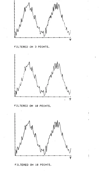
The filtering effect indicated by relation 11 is illustrated in figure 1. It appears clearly that the most active scales of turbulence, in terms of dispersion, increase with elapsed time. A possible consequence of this effect will be analyzed later on.
3 . 4 The random walk approach
While references to this approach are mentioned in the literature and used in some applications (Refs. 2, 3 3 ) , probably the most complete analysis is that made by Durbin ( R e f . 1 2 ) . In the referred paper almost all the relevant aspects are dealt with and the brief description given here only represents a simplified description.
Values of C(x,t) as given in equation 1 can be
obtained by generating random walk for particles from a fixed source or to a fixed observation point. The description here will be very limited and it will not deal with all the subtle ties nor with all the mathematical requirements necessary to provide an exact proof.
In a random system particle trajectories may be compu ted in a discretized way at successive constant time increments At, using what is known as the "drunkard walk", that is using random number generators. This drunkard walk has been
extended by Wiener to continuous system. If AW is a random walk having the value AW. at time t, the value at Τ = NAt is given by :
Ν
WT = Σ A Wn A f
n nAt discrete system (13)
dW.
continuous systemThe AWt must have a certain number of properties, namely that
they are independent of one another and statistically identical
In this case, for the central limit theorem the
probability density distribution of WT will tend to be Gaussian
If Y(t) is the trajectory of a particle it can be computed in such a system as the solution of the equation :
dY(t) = a ( Y ) d Wt (14)
subject to a certain number of conditions (Ref. 1 2 ) .
If one is interested in evolution in terms of time then a normalization can be made by assuming :
dw
t= 0
and
(dW.r =
dt.
Equation 4 can be solved numerically, for large enough samples of dW and time s
of the dispersion
of dW and time steps, to obtain the statistical properties
From equation 14 it is evident that
7 ( t ) = a(Y) d~Wt Ξ 0
while the v a r i a n c e , or typical cloud size is of the type (wi th a = const. ) :
so within these limits this represents (see previous s e c t i o n s ) a pure diffusion phenomenon. The extension to deal with the finite correlation of velocity fluctuations is analyzed in reference 12.
Also in non homogeneous t u r b u l e n c e , the mean velocity (in a Lagrangian sense) may be different from zero. This may be accounted for by modifying equation 14 to become :
dY(t) = b(Y)dt + a(Y)dW (16)
The meaning of a and b is somewhat similar to the Lagrangian displacement velocity as defined by Batchelor and discussed in reference 29.
T h e n , if the dispersion takes place in a flow with mean velocity U ( y ) , the longitudinal displacement can be computed as :
dX = U(Y)dt.
This approach is less often used than the o t h e r , so examples of application are illustrated. One is given, by com-parison, in Appendix 1, two others are briefly discussed here. The first o n e , over-simplified because of the small number of time steps and "markers" used, involves a source at ground level. The surface is considered as fully reflecting in the sense defined
in reference 12. Figure 2 represents the concentration at various tiles in a homogeneous flow, that a a = const, b = 0.
In figure 3 are the results for a "homogeneous shear" flow, where the diffusivity is n = K ( y + y0) , so similar to relation
So in both cases the time shown in the figure could be replaced by the travelled distance χ = U«t.
The density of points plotted is the "representation" of the local c o n c e n t r a t i o n , and the solid line shown represents the position of the cloud centroid.
The appeal of the method for such computations is e v i d e n t , even with the limited number of points used.
A practical drawback is shown by contrast in figure 4 w h e r e the final position of the cloud (for similar condition as
in previous cases) is shown and where the same diffusivity is used but the mean velocity is : U = C χ + C2y (a crude represen
tation of a gradient l a y e r ) .
The limited number of markers used is now so dis persed that it becomes difficult to evaluate a mean value of concentration at each position ( x , y ) .
It should be stressed that this is not a defect of the approach; simply it indicates that a very large number of markers (and of c o m p u t a t i o n s ) should be used to obtain a useful
result. This may be in fact the practical limitation on the usefulness of this t e c h n i q u e , and is in a sense a pity because this seems one of the best suited approach
of dispersal of buoyant (or heavy) gas. It should be hoped that such limits may be o v e r c o m e .
What is measured is the spread from a line source of ground level and at some height inside a boundary layer. Heat is used as a tracer, but the temperature differences are kept low so that this can be considered as dispersion of neutral
contai nment.
Comparisons of the experimental results with the
theoretical ones are shown in figures 5 for the position of the centroid and in figures 6 for the concentration (temperature) profiles in dimensionless form. It can be seen that the agree-ment of the two is pretty good and further work suggests that even more difficult situations can be treated with equally satisfactory results. This seems to apply in particular to the three dimensional source of reference 8.
It should be stressed, however, that the satisfactory results obtained are also due to a useful implementation of the theory in a numerical code. This is essential if the already mentioned limitations due to the finite (and relatively small) number of particles used are to be overcome, and requires a
careful definition of the control values over which the averages are taken and of their evolution with distance.
3.5 The effect of molecular diffusivity
In all the above derivations it is assumed that the particle retains its relative concentration C ( x0) . This means
that all molecular diffusivity phenomena can be neglected. This may not always be the case, so it is important to have a rough
indication of its importance.
feature, so it can be expected to act only at a level compar
able, at most, to the microscale of the turbulent flow field,
λ, and over distances of the same order (Refs. 2,27).
Turbulent transport in contrast, at least for its
dominant features, may be associated with the macroscale L of
the flow. So the relative importance of the two phenomena is
given by the ratio
z/l.
As well as for the case of turbulent
versus laminar viscosity a ratio can be found of the type :
_t
ι
-±
= VRe
V
for the diffusivity one obtains
t = 7P~i
λ
where the Peclet number is given as
Pe =
u'L
u' being the variance of the velocity fluctuations
A
very
deep analysis of the problem is given in
Tennekes & Lumley, and the result indicates that molecular
phenomena can be neglected if (Pe)
case in atmospheric flows.
4. STATISTICAL PROPERTIES OF THE CONCENTRATION
4.1 The probability density function
From what was said before it should be evident that the "instantaneous" concentration at given point in space and time, C ( x , y , z , t ) , should be a random variable, because it is in itself the result of a random series of e v e n t s .
Hence one will require the tools to describe such a variable in a c o n c i s e , but nevertheless comprehensive way. Up to now the only statistical values introduced were the mean v a l u e s , the v a r i a n c e , and the average cloud spread.
A useful description of a stationary variable can be obtained by means of its power spectral d i s t r i b u t i o n . This is very important in terms of turbulence modelling and provides a deep understanding of the phenomena involved.
However, in the context of pollutant dispersal a more useful description of C is in terms of its probability density d i s t r i b u t i o n , p . d . f . In terms of our description of concentration the p.d.f. determines the probability of a tra-jectory passing infinitesimally close to a given point
(Ref. 1 2 ) . In the general case this p . d . f . is function of position in the fluid and time. Alternatively (Ref. 12) it can be said that if a large number of markers are released
from a source then the p . d . f . gives the fraction of t h e s e , that at a fixed time are in a small volume around a given point. By making use of conditional averages it is possible to deter-mine the p . d . f . , and its transport equation from a d e s c r i p t i o n as given in § 3.4.
C o n s i d e r i n g a u n i d i m e n s i o n a l f l o w f o r s i m p l i c i t y one o b t a i n s :
iE + i.
3t
syv- in.
3yJ
3
ay
if.
ayj ( 1 7 )
where Ρ indicates the p.d. function.
The similarity with the gradient diffusion equation for C is e v i d e n t . There is nevertheless one extra term
in-dP
eluded in the convection term : instead of V — one has to
3y
to include the effect of the diffusion itself as — . The 3y
result is that in a non linear problem the shape of the p.d.f. is modified as a function of the non homogeneity of the
diffusivity (as opposed to what happens in most linear mechani cal systems in random vibration a n a l y s i s ) .
The term — 1 plays in the Eulerian framework the
ay]
role of convection velocity. It can also be shown that it
is related to the parameters a and b of section 3.4 by the very simple relations b = V and a2 = 2n. Again reference can be made
,to the formulation quoted in reference 29, for the "meaning of this velocity. When the mean convection is equal to zero (as it
should be in the case of "homogeneous shear" flow discussed in the e x a m p l e ) , then b = a2. This is the way in which the cons
tants were determined in the quoted example.
4.2 Some practical problems related to p.d.f.
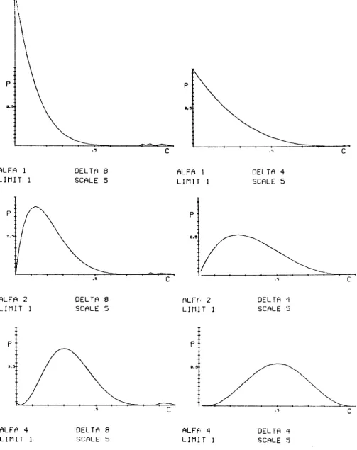
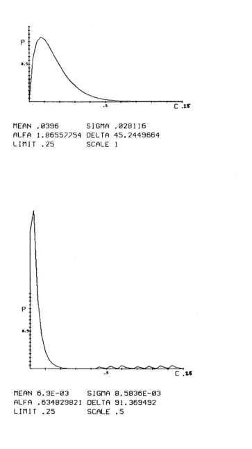
The p . d . f . is expressed by considering the probability of C ( x , t ) being smaller than a fixed value θ :
The range of Ρ is from 0 to 1. Furthermore, C is a bounded v a r i a b l e , 0 < C < 1, and so is θ.
The probability density is the likelihood of C(x,t) being in the range θ-δθ < C < θ + δ θ , so it can be obtained as the derivative of Ρ with respect to θ as :
ρ(θ) =
iE
9Θ
and
p(e)de = 1; p(e)deFor a random variable ρ(θ) h a s , typically, a
Gaussian distribution. In the case of concentration it must also satisfy the condition that ρ(θ) Ξ 0 for θ < 0 and θ > 1.
The importance of the p.d.f. in analyzing the hazard associated with the value of the concententration at a given point and time is now fully recognized. It is evident that in most cases the "mean value" (whatever its definition) is almost
irrelevant. A flame can be ignited at a given point even if C is outside the limits of f l o w a b i l i t y , if it happens that at a certain moment its "instantaneous value" is within the above limits and at the same time there is a source of ignition. In the same way toxic levels may be exceeded if one happens to be at a given point when the "instantaneous concentration" is above a fixed value at a certain time or for a number of times (accumulated e f f e c t ) , no matter what is the mean value at that point. Practical mathematical formulations of this problem have been made by different a u t h o r s ; an extensive example is made in reference 27 and there is no need to repeat it h e r e . For the case of the flame ignition a very good example is the experiments performed and reported in reference 27 by Birch. Fig. qualitatively illustrates a typical result (it should be added that for this particular case Birch was able to explain the results by making use of the p.d.f. of c o n c e n t r a t i o n , but
One point which needs to be added is that the likelihood of an "unwanted situation" does not depend only on the p.d.f. of c o n c e n t r a t i o n , but also on the probability that there is some triggering phenomenon sensitive to it (in other words it will be immaterial to have a toxic concentration level if there is no "observer" there likely to be a f f e c t e d ) . This requires the introduction of the joint probability of two events : for
example that there is a given value of concentration, and simul-taneously that the conditions at that point are such that it may result in damaging e f f e c t s . The second condition is also likely to be, in most practical s i t u a t i o n s , a random v a r i a b l e , described by its own p r o b a b i l i t y .
So the final hazard will depend not only on the p.d.f. of C, but also on the p.d.f. of the (let us say) "situation". Hence the likeliness of the final hazard could be expressed in terms of the joint p.d.f. :
Pj - Pjfcs)
Unless what we called for simplicity concentration (C) and situation (S) are statistically independent variables there is no direct way of determining P. from the individual p.d.f. of the two.
There is enough good e v i d e n c e , experimental and theo-retical to justify the assumption of a Gaussian shape for the p . d . f . in homogeneous turbulence and the fully developed tur-bulence in other flows (Refs. 3 4 , 3 8 ) . This will solve (or at least s i m p l i f y ) the problem if it were not for the fact that
The second exception happens when the shear flow of interest develops in an environment which is not stationary, or affected by a random component. To treat this will require to solve the relevant equations (at least those of the gradient diffusion type) for stochastic boundary condition. Such an attempt is made in reference 1, but it also shows that it is almost impossible to arrive at a general type of solution. Hence some form of phenomenological approach is the best alter-native, at least from a practical standpoint. One of the most often quoted examples of such a phenomenon is the so called "meandering" of plumes,or puffs,of pollutant.
However, it is our opinion that in most situations (including situations where buoyancy plays a predominant r o l e ) , the distinction between meandering and intermittency is a very thin one. Except when the scale (or time) of such phenomenon is large in comparison with the typical plume dimensions (and because this dimension increases with time elapsed, the scale of the external perturbation should be larger and larger as the distance from the source i n c r e a s e s ) , there is no obvious way to make a clear cut distinction between the effects of large flow eddies (a stationary feature of the flow) and the effect of so called "external random perturbation".
Even if the curve in figure 1 may be of some help in trying to decide where to place the limit, one should admit that the distinction will never be a clear cut one.
b e h a v i o u r . Considering the previous remarks on possible use of the p.d.f. for the determination of hazard this point seems to be of outmost interest.
5 · EFFECTS OF MEASUREMENT INSTRUMENTS
5 .1 The sensor effects
A problem always associated with all evaluations of experimental results and also with their comparison to t h e o r y ,
is that the measured value may be different from the ideal o n e .
The point raised here is not that of the errors which are (or could be) associated with any m e a s u r e m e n t , but rather a matter of d e f i n i t i o n .
In a theoretical approach an "infi nitesimally small value around a given point", means that the dimensions c o n s i dered tend; to zero and, as an e x a m p l e , the value of the c o n c e n tration at one point at a given time really means at χ and t, and not at ( X ± A X ) and ( t ± A t ) , no matter how A X and At are small.
In practice any instrument is limited in its p o s s i b i lity to give a value of a quantity in the sense defined b e f o r e . The spatial dimensions(be it a length, a s u r f a c e , or a v o l u m e ) over which is making the measurement (and the time d u r a t i o n ) can be small, but they are almost inevitably finite.
This will be completely irrelevant if the quantity to be measured is uniform and steady, but not if one is in presence of space and time g r a d i e n t s . It is almost trivial to say that the extent of the problem will be dependent on the relative dimensions of the probe and of the scales associated with the variation of the quantity to be m e a s u r e d .
The result is that the probe will be making a sort of averaging of the spatial and time v a r i a t i o n s over its d i m e n s i o n s
The first one which comes to mind is the possible i n t r u s i v e effect of the probe on the quantity to be m e a s u r e d . If the probe, or for that matter its support or any other element, is so large as to m o d i f y the flow field, then one will be measu-ring not only an averaged v a l u e , but an average of values which are m o d i f i e d by the presence of the probe itself. This consi-deration is so obvious that it will not be discussed here. F u r t h e r m o r e , it is so dependent on the interaction that it will be impossible to treat in general t e r m s .
A second e f f e c t , which is related to the a b o v e , and which is of p a r t i c u l a r importance in the field of concentration m e a s u r e m e n t s is the one related to the fact that in some cases probes are not just "sensing" the flow properties but require samples to be taken for a n a l y s i s . The sampling may be continu-ous or in the form of finite burst. If one is interested, as in the present c a s e , in time dependent m e a s u r e m e n t , then only the first case has to be c o n s i d e r e d .
H e r e , with the possible exception of truly isokinetic p r o b e s , it is d i f f i c u l t to e v a l u a t e the value of the flow domain which influences the sensor r e s p o n s e ; the path to the "sink" produced by the probe is different depending of the flow condi-t i o n s . A l s o , icondi-t is difficulcondi-t condi-to evaluacondi-te condi-the effeccondi-t of such mode of action on f l u c t u a t i o n s with time of the quantity to be m e a s u r e d .
the response delay is related to the value of the quantity to be measured or to any other quantity determining the field of interest (such as velocity or p r e s s u r e , in the case of measu-rement of concentration, for e x a m p l e ) .
The last point is related to the threshold of sensiti-vity of the probe itself. That i s.measurements may be impossible or unreliable when the value to be measured is below a certain small value. This is not so much a problem in itself, if this value is small, but raises the problem of the effect of the back-ground level, or of the level of reference. By this we mean the fact that the background level of, say, concentration, is so small as to be undetected; but if the concentration suddenly jumps above the threshold level, then an output is present, which does not represent the actual increase in concentration» being interpreted as referenced to a zero value. It is true that in many cases this question (Ref. 28) is unimportant, but it should not be neglected for instance in the case of toxic gases, as opposed to the case of explosion hazard.
Coming back now to the determination of sensor response it is important to make a distinction between conditions in
which the measurements are carried out.
The essential difference to be considered h e r e , and this point has to be stressed, no matter how many times it has already been discussed, is between stationary and non stationary
behaviour.
as stationary if it is so over a time much larger than the time required to make all the necessary m e a s u r e m e n t s .
The concept of stationarity in time could be transla-ted to its equivalent in space, and in this case one speaks of h o m o g e n e i t y . The same considerations made before,for time
dependence ,can then be translated in terms of space d e p e n d e n c e . H o w e v e r , while there is a large number of flow conditions of practical interest which can be considered as stationary, the number of practical situations in turbulent flows where the condition of homogeneity could be applied is much more limited.
In the domain of pollutant dispersion the classical examples of stationary and non stationary situations are the dispersion of a continuous plume, as opposed to that of a puff from an instantaneous source.
It is a matter of fact that in most cases of interest one has to consider that the problem to be analyzed is time
d e p e n d e n t . This applies in particular to the heavy gas dispersal test (and to most accident-release s i t u a t i o n s ) .
The extent to w h i c h , in practice, the dispersion of a plume from a chimney can be considered as stationary may be the object of some d i s c u s s i o n . In fact the source itself is constant,
but the e n v i r o n m e n t into which it disperses cannot always be considered as such. An example of such an effect is the change in m e t e o r o l o g i c a l c o n d i t i o n s , such as wind velocity and/or
d i r e c t i o n . The limit here is again fixed by the rate at which such change takes place with respect to the observation time. To make a trivial e x a m p l e , if the environment is the same, the plume development under the action of a steady north wind will be the same as for the same plume under the action of a
aligned to its mean value. This raises1, (or can be interpreted
in terms of) the question of absolute versus relative diffusion discussed e l s e w h e r e . However, the author feels that this should not be extended too much to cover for instance the meandering problem, which taken in its strict definition should probably be considered as an inherent feature of turbulence.
On the other hand, one may ask the question of the possibility of making time dependent phenomena look like a
stationary one. This question is possibly less "naive" than it seems, because of the way in which statistical properties are defined for the t u r b u l e n c e . In fact, if one is allowed to re-peat the same time dependent experiment a large number of t i m e s , under identical external c o n d i t i o n s , then averages could be
made, at given (x,t),from the results of the ensemble of e x p e r i -m e n t s . This is precisely the way in which "averages", which are in fact "ensemble averages", are defined for turbulent q u a n t i t i e s . Time averages used in substitution are only an easier way to deal with the problem and justified by the e x i s -tence of an ergodicity theorem.
So, in theory at least, there is no essential
difference between the stationary and time dependent p h e n o m e n a . The problem is that it is almost impossible to reproduce the experiment under identical conditions,and second that the
number of tests required should be so large to make it virtually impracti cal.
The conclusion is then probably that one must consider all the problems of interest here as time dependent, and c o n s i -der all instrumentation problems in this context.
The fact that we consider all the phenomena as time dependent is important in defining the response of the sensor because it makes impractical the use of the spectral represen tation and of the associated Fourier transform and transfer func tion in a straightforward m a n n e r . This is not to say that this is impossible or unjustified, because recourse could be made to so called "instantaneous spectra", or to a description of the time/frequency/amplitude domain (a technique widely used in speed analysis for instance, and more recently in the research in coherent structure in t u r b u l e n c e ) , but that the approach could be too complex to be justified (Ref. 3 9 ) .
One advantage of these descriptions is that in some cases they are reversible (if the transfer function of the instrument is fully known) so that under some conditions it is possible to obtain the real value from the measured one. How ever, this applies in a simple way only for situations dependent on a single variable and their interest will decrease in any case when applied to the four dimensional problems of interest here.
A very interesting analysis of this problem is to be found in reference 36 which investigates the response of hot wire anemometers in turbulent flow field.
On the other hand, an often accepted relationship between the real and measured values is the one given in reference 27 as
w ( x ' , t ' ) A ( x ' ,t')dV(x')dt'
Am
(18)w(x' ,t)dV(x') dt'
weight that the sensor gives to the local value of A, and is
also function of the sensor. The integral at the denominator
simply helps in normalizing the results.
The averaging effect of the above relationship on the
quantity to be measured is self evident, as it is a fact
that there is no way of reconstructing the true A(x,t) from the
measured one. However, it seems also that it is based on a sort
of superposition of effects, that is the result of the sum of local
values of A and w over the value of the transducer, and gives
no immediate indication of the sensor size on the result.
The result is then a fluctuating variable A
m3
m
(dampened in time and space), to which statistical considera
tions could be applied for the computation of mean value,
variance, etc. A couple of points are also discussed in
reference 28, in relation to this, to which we will come later.
However, for further appreciation of the effects of
the sensor on the measured value, it is useful to tentatively
try to evaluate directly its effect on the variance of A. This
will be done simply for a one dimensional case.
If A(x,t) is a fluctuating quantity acting on a sensor
of dimensions
ι
then, assuming w Ξ 1, one obtains :
V*·
1
)
'\
A(x,t)dx
(19)
For the variance of A , one must take into account the concept
m
rm
or if
il
ι
2>
00
ΑΧ = Χ'Χ"
Α(χ' ,t)dx
,A(x",t)dx" = a„,(
x»t)
a! = 2 i
m
2 J (AAX) A(X,t)A(x+AX,t)dAX(20)
The product A ( x ) A ( x + A x ) , averaged, is the spatial autocorrela
tion of the function A =
R ( A X ) .Obviously to go further one requires an expression
for the autocorrelation ( x ) . The choice of an expression of
the type
R(x) = f(*>
has the drawback that it is based :>n the macroscale L of the
f1uctuations,while one is more intîrested here in the effect
of small scale perturbations. In cjmparison to £, (in
general) L could be expected to be much larger.
To take a very simplifie! approach one may consider
as reference the Taylor microscale of turbulent fluctuation λ (in
a
very
crude way one may express tie relationship between λ and
1/2
L as
ι
* L Re
) . Then the autocorrelation near the origin
can be expressed,in a power series development,as
R ( A X )
= a
2Ax
21
(21)
The integral in 20 can then be solved for two condi
tions, namely £ « λ, using relation 21 and £ » λ taking
R ( A X ) = a
2over the length of the integration.
This results in
= a'
αλ ί « λ
(22)
m
a
2L
. 2£ » λ
(23)
The two results are plotted in figure 8, with the dotted line
representing the approximate expected behaviour over the full
range of £/λ values.
In laboratory conditions it is not unusual, or at
least not impossible that the situation is close to case one,
w\hile in most practical application the second situation may
be more likely.
In this context λ can be assumed as a typical dimen
sion over which the quantity to be measured is extremely well
correlated, that is the dimension of fluid pockets inside which
it can be assumed to be practically constant.
It is easy to see that for the ratios £/λ of the order
of 10 the effect is already very large (however, it should be
noted that the Taylor microscale £ is larger than the
Kolmogo.-off microscale often given as a reference value).
It should be noted, however, that to obtain the
results one had to consider the likelihood of the simultaneity
of the events on the length of the probe: this had led to
equation 18 which i^ averaged with respect to time so while a
2- o m
To illustrate this one can make a single example : consider that a pocket of fluid is convected with velocity U over the probe for a time At. Inside this pocket (of dimen-sion U « A t « £ ) , the containment (quantity to be measured) may be contained, with concentration 1, over 25% in a single lump, or, also with concentration 1 in a large number of smaller lumps also accounting for 25% of the total. Also the position of these lumps may be different within U«At«£. The real values of concentration are always either 0, or 1. The measured values will change as function of the above quoted parameters. The average measured will always be 0.25. In contrast, the
measured values of the variance (evaluated over At) will be d i f f e r e n t , depending on the relative position of the lumps, as indicated schematically in figure 9.
Over the time At (and assuming a perfect time res-ponse for the probe) in cases (1) the measured variance is 0. In case (2) the measured variance should coincide with the real one. In case (3) it is smaller than the true one while in 4 it tends to 0 again. The above is a very sketchy illustration but indicates how the distribution of high concentration pockets in time and space may combine to an unrealistic measured value. The situation extended to the four dimensional case will look even more complex, but substantially not different : only in the case where the equal concentration lumps are larger than the four dimensional region sensed by the probe will there be an agreement in the results : the only situation which satisfies this condition in the figures is the case 2.
5.2 Analysis of results
action of the s e n s o r ) . If a wave number could be defined as the inverse of space dimensions
K = — (24)
then it could be expected that for wave number below K as
defined above the effect will be small, while for K above that the attenuation will be increasing with it. This is schemati-cally shown in figure 1 0 . The situation is in fact more complex because one has to take into account the three dimensional
nature of K (which is a vector in turbulent flow fields) and the effect of time. (Ref. 36)
Nevertheless, it could be said that, to generalize, the high frequency (both in space and time) components will be dampened or smoothed, and even more important the high
level short duration spikes reduced in amplitude and deformed. Now toward the edges of a cloud of contaminants (to return to the problem of interest h e r e ) , these spikes are a dominant feature of the problem (because of the low value of the inter-mittency factor h e r e ) , the elements which contribute to the
typical twin peak shape of the probability density distribution. So one may expect that in this region there is a large likelihood of having a substantial difference between the true and the
measured statistical quantities describing the concentration behaviour.
If the measured p.d.f. is not correct then all the statistical values associated with the concentration at a given point are likely to be affected, including the mean value. This is meant to say that the mean value is not reduced to the value of concentration averaged over the probe value (instead of the local o n e ) , but also that it can be lower than it.
of the p.d.f. So the ratio of external value to variance
(also underestimated) may be substantially smaller when computed
from measurements, than expected from theory. The same
consi-deration applies to skewness and flatness (third and fourth
moment of v a r i a n c e ) .
It goes without saying that the above conclusions are
of importance when estimating the likelihood of having, for
example, the concentration falling into the limits of
flammabi-1 i ty, or when trying to estimate the instantaneous or
cumula-tive toxicity levels.
Two last points need to be mentioned for their effect
on the measured one. The first is the non linearity of the
response of a probe. The fact that when measuring a fluctuating
quantity,the statistical values computed from the output do not
coincide with the real one,should be considered as trivial,
because if the calibration curve is known then "linearizing"
the results before using them fully solves the problem and
should always be applied. The second is much more critical
and is the fact that the values of the weighed function w in
equation 18 (and following) may be a function of the local value
of the quantity to be measured. This is an almost intractable
problem, but not unusual; to quote as examples two widely used
instruments, it plays a certain role in the response of hot
wire anemometers and to some extent in laser doppler velocimeter
(the bias effect may be considered as a form of this phenomenon)
Few attempts have been made to analyze in full the problem
in the general form. It should be stressed, however, that
whenever possible a check should be made of its possible
existence on the particular probe to be used.
by measurement errors as mentioned above, one may raise the question of how much the models themselves are biased by this effect. On the basis of the treatment of specific theoretical flow (like isotropic turbulence) and considering the accuracy which can be achieved in laboratory m e a s u r e m e n t s , the above points should not be considered as the biggest worry at the moment in this domain. On the contrary it is true to say that new experimental techniques have put into perspective flow properties (like the existence of coherent structures) which were previously neglected in all theoretical approaches.
It should be stated, however, that attempts have been made to rewrite the equation for containment dispersal»based on measured values. This will usually lead to more complex
formu-lations which will not be discussed here. A good account of this is given in reference 27.
In the above c o n s i d e r a t i o n s , recourse had to be made to time a v e r a g e s , an approach which may be unacceptable in the analysis of time dependent phenomena. In an unsteady situation the evolution of A(x,t) may be like in figure 9 with the
measured counterpart shown as A ( x , t ) . The smoothing takes
mx '
place both because of volume and time averaging in the probe, so the mean and all the other statistical parameters are likely to be different. But the problem always remains of how to
determine the statistical values associated with such a curve. In other words to determine what is, say,the evolution of the mean value of A(x,t) with time, if such a quantity can be
defined. The point is raised because most of the simpler models predict the evolution in time of such mean values : for instance the evolution in time at a given point in space of the concentration associated to the passage of a puff release .
It is also evident that such a problem will not arise, or at least could be easily solved if one had available a large number of samples, such as those in figure 11, coming from indi vidual but statistically independent tests. In such a case, recourse could always be made to ensemble averages, which, as said before, are the proper way to deal with such a problem. Also, a solution will be possible if results are available from non identical but sufficiently similar tests, but presented in the form of relative dispersion. The aspect of relative
dispersion is dealt with in detail in reference 27, and, to summarize»simply consists of presenting the data from each test referred to the centroids of the puffs computed at equivalent times.
Neither of the above proposals is easy to put into practice, at least for full scale tests, because of the large number of the required experiments to be performed.
The above considerations are made assuming that one is following the development of a puff from an instantaneous point source, and which is convected away by a mean flow velo city over distances large in comparison to its typical dia meter (which can be conveniently defined as the value of σ as a function of time).
For the case of releases in no wind conditions and measurements at relatively small distances, the figure may be
interpreted as typical of the arrival at the sensor of the cloud front. This is a close representation of a number of full
scale tests. All the considerations made before still apply, but another approach is now possible, even if the limits of its applicability have to be carefully considered for each case.
This will be to make averages of results obtained along different