Vol. 10 (2016) 3693–3722 ISSN: 1935-7524
DOI:10.1214/16-EJS1209
Convergence and rates for fixed-interval
multiple-track smoothing using
k
-means
type optimization
∗
Matthew Thorpe
Department of Mathematical Sciences Carnegie Mellon University
Pittsburgh PA 15213
e-mail:[email protected]
and
Adam M. Johansen
Department of Statistics University of Warwick
Coventry CV4 7AL
e-mail:[email protected]
Abstract: We address the task of estimating multiple trajectories from unlabeled data. This problem arises in many settings, one could think of the construction of maps of transport networks from passive observation of travellers, or the reconstruction of the behaviour of uncooperative vehicles from external observations, for example. There are two coupled problems. The first is a data association problem: how to map data points onto indi-vidual trajectories. The second is, given a solution to the data association problem, to estimate those trajectories. We construct estimators as a solu-tion to a regularized variasolu-tional problem (to which approximate solusolu-tions can be obtained via the simple, efficient and widespreadk-means method) and show that, as the number of data points,n, increases, these estimators exhibit stable behaviour. More precisely, we show that they converge in an appropriate Sobolev space in probability and with raten−1/2.
MSC 2010 subject classifications:62G20.
Keywords and phrases:Asymptotics,k-means, non-parametric regres-sion, rates of convergence, variational methods.
Received October 2015.
∗Part of this work was completed whilst MT was part of MASDOC at the University of Warwick and was supported by an EPSRC Industrial CASE Award PhD Studentship with Selex ES Ltd. The authors would also like to thank Neil Cade (Selex ES Ltd.) and Florian Theil (University of Warwick) whose discussions enhanced this paper as well as Riccardo Cristoferi (Carnegie Mellon University) for feedback on an earlier version of the manuscript. The authors also gratefully acknowledge the feedback of the referee whose comments significantly improved this manuscript.
3694
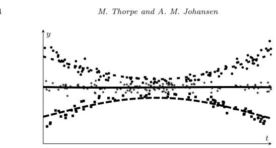
Fig 1. Unlabeled data is generated from three targets and using minimizers of (2) we can
find a partitioning of the data set and nonparametrically estimate each trajectory using the k-means algorithm.
1. Introduction
Given observations from multiple moving targets we face two (coupled) lems. The first is associating observations to targets: the data association prob-lem. The second is estimating the trajectory of each target given the appropriate set of observations. When there is exactly one target the data association prob-lem is trivial. However, when the number of targets is greater than one (even when the number of targets is known) the set of data association hypotheses grows combinatorially with the number of data points. Very quickly it becomes infeasible to check every possibility. Hence fast approximate solutions are needed in practice.
In this paper we interpret the problem of estimating multiple trajectories with unknown data association (see Figure1) in such a way that thek-means method [32] may be applied to find a solution. As in [42], this is a non-standard application of thek-means method in which we generalize the notion of a ‘cluster center’ to partition finite dimensional data using infinite dimensional cluster centers. In this paper the cluster centers are trajectories in some function space and the data are space-time observations.
Let Θ⊂(Hs)k whereHsis the Sobolev space of degrees(where we consider
the case s ≥ 1, see Section 2.1 for a precise definition). We have a data set
{(ti, yi)}in=1⊂[0,1]×Rd and a model for the observation process
yi=μ†ϕ(i)(ti) +i (1)
where μ† = (μ†1, . . . , μk†) is some unknown function, i iid∼ φ0 and ti iid
∼ φT for densities φ0 and φT on [0,1] and Rd respectively. We assume that the index
of the cluster responsible for any given observation is an independent random variable with a categorical distribution of parameter vector p = (p1, . . . , pk),
writing ϕ(i) ∼Cat(p) to mean P(ϕ(i) = j) = pj. This assumptions allow us
[image:2.612.176.450.86.233.2]denote byφY(y|t), as
φY(y|t) =
k
j=1
pjφ0(y−μ†j(t)).
We can summarize the stylized data generating process as follows. A cluster is selected at random: P(ϕ =j) =pj, the time and observation error are drawn
independently from their respective distributions, t∼φT, and∼φ0; and we observe (t, y=μ†ϕ(t) +).
The aim is to estimateμ†= (μ†1, . . . , μk†)∈Θ from observed data{(ti, yi)}n i=1. In particular the data association
ϕ:{1,2, . . . , n} → {1,2, . . . , k}
is unknown. With a single trajectory (k= 1) the problem is precisely the spline smoothing problem, see for example [46]. Fork >1 trajectories there is an ad-ditional data association problem coupled to the spline smoothing problem. We call this the smoothing-data association (SDA) problem. Although the estima-tor μn we propose is not necessarily a consistent estimator forμ† (we do not show μn→μ†) we do consider our estimator a natural choice. We believe it is possible to bound the asymptotic error limn→∞μn−μ†(L2)k ≤C where C
depends on the distribution of the data points, however it is beyond the scope of this work to show such a bound. We refer to [28, Section 4.5] for a bound of the type μ∞−μ† ≤ C, where μ∞ = limn→∞μn, for k-means in Hilbert
spaces.
We assume k is fixed and known. The aim of this paper is to construct a sequence of estimators μn of μ† based upon increasing sets of observations {(ti, yi)}n
i=1 and to study their asymptotic behavior as n→ ∞. For eachnour estimate is given as a minimizer offn: Θ→Rdefined by
fn(μ) =
1
n n
i=1
k
j=1
|yi−μj(ti)|2+λ k
j=1
∇sμj2
L2 (2)
where | · | is the Euclidean norm on Rd, kj=1zj = min{z1, . . . , zk} andλ is a positive constant. Penalizing thesth derivative ensures that the problem is well posed. Optimizing this function can be interpreted as seeking a hard data asso-ciation: given μ∈ Θ each observation (ti, yi) is associated with the trajectory
closest to it so the corresponding data association solution is given by
ϕμ(i) = argmin
j=1,2,...,k
|μj(ti)−yi|.
3696
of parameters (which will perform poorly when those assumptions are inap-propriate) or to proceed nonparametrically, optimising a cost function which balances the trade-off between a good fit to the data and regularity of the so-lution (which requires the precise specification of the notion of regularity). In this paper we pursue the second route, showing that in the large data limit the proposed estimators behave well. The main contribution of this paper is to establish the stability ofk-means like estimators to the SDA problem.
Although exact solution of the underlying optimization problem is NP com-plete even in benign Euclidean settings [17], the computational cost of iterative numerical approximation has been shown to have a polynomial (smoothed) cost in certain Euclidean settings, e.g. [3], and in practice the performance is often much better than these bounds would suggest: it is accepted to be a numerically efficient method for obtaining approximate solutions (i.e. local minimizers). Our empirical experience is that this property holds also within the context consid-ered by this paper. Our focus is upon the asymptotic properties of the ideal estimator and it is beyond the scope of this paper to upper bound the com-putational complexity of the numerical iteration scheme. We do however point out that a key advantage of thek-means method is that it reduces the problem of solving the multiple target problem (k > 1) to the problem of repeatedly solving the single target problem (k= 1) which can be done efficiently with, for example, splines.
There are of course several variations of the k-means method, e.g. fuzzy
C-means clustering [6] (a soft version of k-means closely-related to the EM algorithm [19]),k-medians clustering [8] (anL1version ofk-means), Minkowski metric weightedk-means [18] for which the analysis, particularly the convergence result in Theorem3.1, could be easily adapted. Indeed, for bounded noise, the weak convergence k-medians clustering is a special case of [42] and to extend the result to unbounded noise one can follow the strategy given in the proof of Theorem 3.4. The strong convergence and rate of convergence will require a different approach as one loses differentiability when going fromL2 toL1.
The choice of regularization scheme and, in particular, ofλis not straightfor-ward. Fork= 1 there are many results in the spline literature on the selection of λ = λn and the resulting asymptotic behavior as n → ∞, see for
exam-ple [1, 11, 12, 13, 29, 33, 37, 38, 39, 40, 43, 44, 45, 47]. In this case one has
λn→0 and can expectμn to converge toμ†. Convergence is either with respect
to a Hilbert scale, e.g.L2, or in the dual space, i.e. weak convergence. Using a Hilbert scale in effect measures the convergence in a norm weaker thanHs. We
remark that whenk > 1 andλn →0 sufficiently slowly we would expect that minimizersμn converge to a minimizerμ∗ of
1
0
Rd
k
j=1
|y−μj(t)|2φY(y|t)φT(t) dydt.
The approach we take, as is common in settings in which smooth solutions are expected, is to penalize thesthderivative. By Taylor’s Theorem we can write
Hs=H
0⊕ H1 where
H0= span
ζi(t) = t
i
i! :i= 0,1, . . . , s−1
,
H1=
g∈Hs:∇ig(0) = 0 for alli= 0,1, . . . , s−1 .
We use · 1=∇s· L2 as the norm onH1 and denote theH0 norm by · 0,
and therefore we use the norm · Hs= · 0+ · 1onHs(which is equivalent
to the usual Sobolev norm). SinceH0is finite dimensional we are free to use any norm we choose without changing the topology. We can view Hs = H0⊕ H1 as a multiscale decomposition of Hs. The polynomial component represents a coarse approximation. The regularization penalizes oscillations on the fine scale, i.e. inH1.
In the casek= 1,fnis quadratic and one can find an explicit representation of μn, i.e. there exists a random function G
n,λ such that with probability one μn =G
n,λνn for some functionνn which depends on the data. Whenk >1 the
problem is no longer convex and the methodology used in thek= 1 case fails. The first result of this paper (Theorem3.1) is a weak convergence result, we show that there existsμ∞∈Θ such that (up to subsequences)μn μ∞a.s. in Hsandμ∞ is a minimizer off
∞defined by
f∞(μ) =
1
0
Rd
k
j=1
|y−μj(t)|2φY(y|t)φT(t) dydt+λ k
j=1
∇sμ
j2L2. (3)
One should note that if μ∞ = (μ∞1 , . . . , μ∞k ) is a minimizer of f∞ then so is ˜
3698
minimum minfn (in infinite dimensional settings) and [27] gives results for the
convergence of the minimizers.
The result of Theorem 4.1 is that, upto subsequences, the convergence is strong inHs. The final result is to show that the rate of convergence is of order
1 √
n in probability. I.e.
μn−μ∞
(Hs)k=Op
1
√ n
.
This is closely related to the central limit theorem first proved for thek-means method by Pollard [36] for Euclidean data. We extend his methodology to clus-ter cenclus-ters inHsto prove our rate of convergence result and in doing so provide a theoretical justification for using this method in the more complex scenario which we consider and, in particular, for using such approaches to address post hoc tracking of multiple targets using k-means type algorithms. As with Pol-lard’s finite dimensional result we require an assumption on the positive defi-niteness of the second derivative of the limiting functionf∞.
In the next section we remind the reader of some preliminary material which underpins our main results. Section3 contains the weak convergence result. In Section4 we go from weak convergence to strong convergence with rates.
2. Preliminaries
2.1. Notation
The Borelσ-algebra on [0,1]×Rdis denotedB([0,1]×Rd) and the set of proba-bility measures on ([0,1]×Rd,B([0,1]×Rd)) byP([0,1]×Rd). Our main results
concern sequences of data {(ti, yi)}∞i=1 sampled independently with common lawP∈ P([0,1]×Rd) which is assumed to have a Lebesgue density,φ((t, y)) = φY(y|t)φT(t). We work throughout on a probability space (Ω,F,P) rich enough
to support a countably infinite sequence of such observations, (ti, yi) : Ω →
[0,1]×Rd. All random elements are defined upon this common probability space
and all stochastic quantifiers are to be understood as acting with respect toP un-less otherwise stated. With a small abuse of notation we say (ti, yi)∈[0,1]×Rd.
We will define the space Θ⊂(Hs)k in Section 3. The Sobolev spaceHs is
given by
Hs:=μ: [0,1]→Rd s.t.∇iμis abs. cts.∀i= 0,1, . . . , s−1 and∇sμ∈L2 .
Note that data is of the form{(ti, yi)}in=1⊂[0,1]×Rd.
We denote weak convergence by: ifνn, ν ∈HssatisfiesF(νn)→F(ν) for
allF ∈ (Hs)∗ then νn ν. A sequence of probability measures P
n is said to
weakly converge toP if for all bounded and continuous functionshwe have
Pnh→P h.
Where we writeP h=h(x)P(dx). IfPn weakly converges toP then we write Pn⇒P.
Definition 2.1. We define the following.
(i) For deterministic sequences an and rn, where rn are positive and real valued, we write an =O(rn) if an
rn is bounded. If
an
rn →0 asn → ∞ we
writean=o(rn).
(ii) For random sequences an andrn, where rn are positive and real valued, we write an =Op(rn) if arnn is bounded in probability: for all >0 there exist deterministic constantsM, N such that
P
|an| rn ≥M
≤ ∀n≥N.
If an
rn →0 in probability: for all >0
P
|an| rn ≥
→0 asn→ ∞
we writean=op(rn).
Whena=a(r) can be written as a function ofrwe will often writea=O(r) or a =o(r) to mean for any sequence rn → 0 thatan := a(rn) satisfies an = O(rn) oran=o(rn) respectively.
2.2. Γ-convergence
Our proof of convergence will use a variational approach. In particular the nat-ural convergence for a sequence of minimization problems is Γ-convergence. The Γ-limit can be understood as the ‘limiting lower semi-continuous envelope’. It is particular useful when studying highly oscillatory functionals when there will often be no strong limit and the weak limit (if it exists) will average out os-cillations and therefore change the behavior of the minimum and minimizers. See [9,16] for an introduction to Γ-convergence and [23,24,42] for applications of Γ-convergence to problems in statistical inference. We will apply the following definition and theorem toH= Θ⊂(Hs)k.
Definition 2.2 (Γ-convergence [9, Definition 1.5]). Let H be a Banach space and Θ⊂ H be a weakly closed set. A sequence fn : Θ→R∪ {±∞} is said to
Γ-converge on Θto f∞ : Θ→R∪ {±∞} with respect to weak convergence on H, and we writef∞= Γ-limnfn, if for all ν∈Θwe have
(i) (lim inf inequality) for every sequence(νn)⊂Θweakly converging to ν
f∞(ν)≤lim inf
n fn(ν n);
(ii) (recovery sequence) there exists a sequence (νn) weakly converging to ν such that
f∞(ν)≥lim sup
n
3700
When it exists the Γ-limit is always weakly lower semi-continuous [9, Propo-sition 1.31] and therefore achieves its minimum on any weakly compact set. An important property of Γ-convergence is that it implies the convergence of minimizers. In particular, we will make use of the following result which can be found in [9, Theorem 1.21].
Theorem 2.3(Convergence of Minimizers). Let Hbe a Banach space,Θ⊂ H
be a weakly closed set and fn : Θ → R∪ {±∞} be a sequence of functionals. Assume there exists a weakly compact subsetK⊂Θwith
inf
Θ fn= infK fn ∀n∈N.
If f∞= Γ-limnfn andf∞ is not identically±∞then
min
Θ f∞= limn infΘ fn.
Furthermore ifμn ∈K minimizes fn then any weak limit point is a minimizer of f∞.
2.3. The Gˆateaux derivative
As in Section2.2we will apply the following toH= Θ⊂(Hs)k.
Definition 2.4. We say thatf :H →Ris Gˆateaux differentiable atμ∈ H in direction ν∈ Hif the limit
∂f(μ;ν) = lim
r→0+
f(μ+rν)−f(μ)
r
exists. We may define second order derivatives by
∂2f(μ;ν, ω) = lim
r→0+
∂f(μ+rω;ν)−∂f(μ;ν)
r
forμ, ν, ω ∈ H. In cases where the second derivative does not necessarily exist we will define∂−2f by
∂−2f(μ;ν, ω) = lim inf
r→0+
∂f(μ+rω;ν)−∂f(μ;ν)
r .
To simplify notation, we write:
∂−2f(μ;ν) :=∂2−f(μ;ν, ν).
Theorem 2.5. Let μ, ν ∈ H. If f :H → R is continuously Gˆateaux differen-tiable on the set {tμ+ (1−t)ν : t∈[0,1]} then
f(ν)≥f(μ) +∂f(μ;ν−μ) +1 2∂
2
−f((1−t∗)μ+t∗ν;ν−μ)
Proof. The theorem is only a slight generalisation of Taylor’s theorem. Indeed, if there existst∈[0,1] such that∂2
−f((1−t)μ+tν;ν−μ) =−∞then we have nothing to prove. So we assume∂2
−f((1−t)μ+tν;ν−μ)>−∞for allt∈[0,1], defineg(t) =f((1−t)μ+tν) then we can show thatg(1) =f(ν),g(0) =f(μ),
g(0) =∂f(μ;ν−μ) andg−(t) =∂2
−f((1−t)μ+tν;ν−μ) where we define
g−(t) = lim inf
r→0+
g(t+r)−g(t)
r . (4)
Hence we can equivalently show that g(1) ≥ g(0) +g(0) + 12g−(t∗) for some
t∗∈[0,1]. DefineJ = 2(g(1)−g(0)−g(0)) and we are left to showJ ≥g−(t∗). Let
F(t) =g(t) +g(t)(1−t) +(t−1) 2
2 J−g(1)
and note that, by definition ofJ,F(0) =F(1) = 0. SinceF−(t) = (1−t)(g−(t)−
J) (where F− is defined analogously to (4)), then if we can show there exists
t∗ ∈ (0,1) such that F−(t∗) ≤ 0 we are done. One can easily show that if
F−(t)>0 for alltthenF is strictly increasing, which contradictsF(1) =F(0), and so there must exist such a t∗.
3. Weak convergence
To show weak convergence we apply Theorem2.3. The following two subsections prove that the conditions required to apply this theorem, i.e. that f∞ is the Γ-limit of fn and that the minimizers μn are uniformly bounded, hold with
probability one.
For a fixed δ > 0 we define the set Θ to be the set of functions in (Hs)k
which have minimum separation distance ofδ:
Θ =μ∈(Hs)k:|μj(t)−μl(t)| ≥δ∀t∈[0,1] andj =l . (5)
For d = 1 this is a strong assumption as we restrict ourselves to trajectories that do not intersect. When considering the tracking of real objects in 2 or more dimensions, the assumption is typically physically reasonable. For example ifμj
are to represent trajectories of extended objects by modelling the location of the centroid, it is natural to require a minimum separation of those centroids on a scale corresponding to the extent of the objects in question.
3702
here. Such a statement would imply that one could carry out the classification using ak-means method without directly imposing the constraint.
We use the assumption in order to infer that the spatial partitioning induced by any set of cluster centers μ∈Θ is such that every element of the partition is non-empty, at every timet, i.e. the sets
Xj(t) =x∈Rd : |x−μj(t)|<|x−μi(t)|fori=j
forj= 1, . . . , k are all non-empty.
First let us show that Θ is weakly closed in (Hs)k. Take any sequenceμn∈Θ
such thatμn μ∈(Hs)k. We have to showμ∈Θ. Pickt∈[0,1],j =l and
defineF : Θ→Rd byF :ν→νj(t)−νl(t), note thatF is in the dual space of
(Hs)k (sinces≥1). Hence
δ≤ |μnj(t)−μln(t)|=|F(μn)| → |F(μ)|=|μj(t)−μl(t)|.
Thereforeμ∈Θ. Furthermore we can show thatfn, f∞ are weakly lower semi-continuous [42, Propositions 4.8 and 4.9] hence they obtain their minimizers over weakly compact subsets of Θ. We will show that minimizers are contained in a bounded, and hence weakly compact set, and therefore there exists minimizers offn and f∞on Θ.
We now state our assumptions.
Assumptions. 1. The data sequence (ti, yi) is independent and identically distributed in accordance with the model (1), with μ† ∈ (L∞)k, ϕ(i) ∼
Cat(p), i ∼φ0, ti ∼ φT: ϕ(i), i and ti are mutually independent, and
(ϕ(i), i, ti), (ϕ(j), j, tj) are independent for i = j. We assume φ0 and
φT are continuous densities with respect to the Lebesgue measure on Rd and[0,1]respectively and use the same symbols to refer to these densities and to their associated measures.
2. The densityφ0 is centered and has finite second moments.
3. For all∈Rd,φ0()>0.
4. There existsα <−d−3 andc1 such thatsupt∈[0,1]φY(y|t)≤c1|y|α. Observe that
fn(μ†) =
1
n n
i=1
k
j=1
|μ†j(ti)−yi|2+λ k
j=1
∇sμ† j
2
L2
≤ 1 n
n
i=1
|μ†ϕ(i)(ti)−yi|2+λ k
j=1
∇sμ† j2L2
= 1
n n
i=1
2i +λ k
j=1
∇s μ†j2L2
→Var(i) +λ k
j=1
∇sμ†
where the convergence is almost surely by the strong law of large numbers. Hence Assumption 2 implies that there exists N such that minμ∈Θfn(μ)< α+ 1 for n ≥ N and N < ∞ with probability one (although N could depend on the sequence{ti, yi}n
i=1 and so we could have supω∈ΩN=∞).
To simplify our proofs we use Assumption 3 although the results of this paper can be proved without it. The assumption is used in bounding the minimizers of fn. Clearly if φ0 has bounded support then each yi is uniformly bounded (a.s.) and one can show that |μn(t)| is bounded uniformly in n and t (a.s.).
Assumption 3 can be relaxed at the expense of some trivial but notationally messy modifications.
Assumption 4 is used the next section to uniformly control the decay in the densityφY. In particular the assumption allows us bound the error due to restricting to bounded sets. Although Assumption 4 implies thatφ0has at least two moments we include the second moment condition in Assumption 2 as the decay in density is not needed until later sections.
Note the second moment condition implies that φ0 decays as|| → ∞ and therefore, by continuity,φ0 is bounded inL∞.
We now state the main result for this section. The proof is an application of Theorem 2.3once we have shown that f∞ is the Γ-limit (Theorem3.2) and established the uniform bound on the set of minimizers Theorem3.4(which by reflexivity of the space (Hs)k implies weak compactness).
Theorem 3.1. Define fn, f∞ : Θ → R by (2) and (3) respectively, where
Θ⊂(Hs)k fors≥1 is given by (5). Under Assumptions 1–3 any sequence of minimizersμn offn is, with probability one, weakly compact and any weak limit μ∞ is a minimizer of f∞.
3.1. The Γ-limit
We claim the Γ-limit of (fn) is given by (3).
Theorem 3.2. Define fn, f∞ : Θ→R by (2) and (3) respectively where Θ⊂
(Hs)k fors≥1 is given by (5). Under Assumptions 1–2
f∞= Γ-lim
n fn
for almost every sequence of observations (t1, y1),(t2, y2), . . ..
Proof. We are required to show that the two inequalities in Definition 2.2hold with probability 1. In order to do this we follow [42] and consider a subset of Ω of full measure, Ω, and show that both statements hold for every data sequence obtained from that set.
For clarity let P(d(t, y)) =φY(dy|t)φT(dt). LetPn(ω) be the associated
em-pirical measure arising from the particular elementary eventω, which we define via it’s action on any continuous bounded functionh: [0,1]×Rd→R:P(ω)
n h=
1
n n
i=1h
t(iω), y(iω)
where
t(iω), yi(ω)
emphasizes that these are the
observa-tions associated with elementary event ω. Define gμ(t, y) = k
3704
To highlight the dependence offn onω we writefn(ω). We can write
fn(ω)(μ) =Pn(ω)gμ+λ k
j=1
∇sμj2
L2 and f∞=P gμ+λ k
j=1
∇sμj2
L2.
We define
Ω=
ω∈Ω :Pn(ω)⇒P
∩ω∈Ω :Pn(ω)(B(0, q)c)→P(B(0, q)c)∀q∈N
∩
ω∈Ω :
(B(0,q))c
|y|2P(ω)
n (d(t, y))→
(B(0,q))c
|y|2P(d(t, y))∀q∈N
then P(Ω) = 1 by the almost sure weak convergence of the empirical mea-sure [20] and the strong law of large numbers.
Fixω ∈Ω and we start with the lim inf inequality. Let μn μ. By
Theo-rem 1.1 in [21] we have
[0,1]×Rd
lim inf
n→∞,(t,y)→(t,y)gμ
n((t, y))P(d(t, y))
≤lim inf
n→∞
[0,1]×Rd
gμn(t, y)P(ω)
n (d(t, y)).
By the same argument as in Proposition 4.8.ii in [42] we have
lim inf
n→∞,(t,y)→(t,y)
y−μnj(t)2≥(y−μj(t))2.
Taking the minimum overj we have
lim inf
n→∞,(t,y)→(t,y)gμ
n(t, y)≥gμ(t, y).
And, as norms in Banach spaces are weak lower semi-continuous,
lim inf
n→∞ ∇ sμn
j2L2 ≥ ∇sμj2L2.
Therefore
lim inf
n→∞ f (ω)
n (μn)≥f∞(μ)
as required.
We now establish the existence of a recovery sequence for everyω ∈Ω and everyμ∈Θ. Letμn =μ∈Θ. Letζq be aC∞(Rd+1) sequence of functions such that 0≤ζq(t, y)≤1 for all (t, y)∈Rd+1,ζq(t, y) = 1 for (t, y)∈B(0, q−1) and
ζq(t, y) = 0 for (t, y)∈B(0, q). Then the functionζq(t, y)gμ(t, y) is continuous for allq. We also have, for any (t, y)∈[0,1]×Rd,
ζq(t, y)gμ(t, y)≤ζq(t, y)|y−μ1(t)|2
≤2ζq(t, y)
|y|2+|μ1(t)|2
≤2ζq(t, y)
|y|2+μ
12L∞([0,1])
≤2|q|2+ 2μ12L∞([0,1])<∞
so ζqgμ is a continuous and bounded function, hence by the weak convergence
ofPn(ω)toP we have
Pn(ω)ζqgμ →P ζqgμ
as n→ ∞for allq∈N. For allq∈Nwe have
lim sup
n→∞ |P (ω)
n gμ−P gμ| ≤lim sup n→∞ |P
(ω)
n gμ−Pn(ω)ζqgμ|
+ lim sup
n→∞ |P
(ω)
n ζqgμ−P ζqgμ|+ lim sup n→∞ |P ζq
gμ−P gμ|
= lim sup
n→∞ |P
(ω)
n gμ−Pn(ω)ζqgμ|+|P ζqgμ−P gμ|.
Therefore,
lim sup
n→∞ | P(ω)
n gμ−P gμ| ≤lim sup q→∞
lim sup
n→∞ | P(ω)
n gμ−Pn(ω)ζqgμ|
by the dominated convergence theorem. We now show that the right hand side of the above expression is equal to zero. We have
|P(ω)
n gμ−Pn(ω)ζqgμ| ≤Pn(ω)I(B(0,q−1))cgμ
≤
[0,1]×Rd
I(B(0,q−1))c(t, y)|y−μ1(t)|2Pn(ω)(d(t, y))
≤2
[0,1]×RdI(B(0,q−1))
c(t, y)|y|2Pn(ω)(d(t, y))
+ 2μ12L∞([0,1])
[0,1]×Rd
I(B(0,q−1))c(t, y)Pn(ω)(d(t, y))
n→∞ −→ 2
[0,1]×RdI(B(0,q−1))
c(t, y)|y|2P(d(t, y))
+ 2μ12L∞([0,1])
[0,1]×Rd
I(B(0,q−1))c(t, y)P(d(t, y))
q−→→∞ 0
where the last limit follows by the monotone convergence theorem and Assump-tion 2. We have shown
lim
n→∞|P
(ω)
n gμ−P gμ|= 0.
Hence
3706
3.2. Boundedness
The aim of this subsection is to show that the minimizers of fn are uniformly bounded innfor almost every sequence of observations. We divide this into two parts; bounding each of the H0 and H1 norms. The H1 bound follows easily from the regularization. For theH0 bound we exploit the equivalence of norms on finite-dimensional vector spaces to choose a convenient norm onH0.
By the argument which followed the assumptions we have, for nsufficiently large and with probability one, minμ∈Θfn(μ)≤α+ 1<∞. Now we letμn be
a sequence of minimizers. Then there exists ˆΩ⊂Ω such thatP( ˆΩ) = 1 and for allω∈Ω we haveˆ
fn(μ†) =Pn(ω)gμ†+λ k
j=1
∇sμ†
j2L2 →P gμ†+λ k
j=1
∇sμ†
j2L2 =:α.
Therefore for allω∈Ω there existsˆ N =N(ω)such that forn≥N we have
λ k
j=1
μn
j21≤fn(μn)≤fn(μ†)≤α+ 1.
Therefore μn
j1 is bounded almost surely for each j. We are left to show the corresponding result forμn
j0.
The following lemma will be used to establish the main result of this subsec-tion, Theorem3.4. It shows that, if for some sequenceνn∈Hswith∇sνnL2 ≤ √
αandνn0→ ∞, then we have that, up to a subsequence,|νn(t)| → ∞with the exception of at most finitely manyt∈[0,1]. When applied toμn
j this will be
used to show that in the limit, if any center is unbounded, then the minimization can be achieved overk−1 clusters — and hence to provide a contradiction.
Lemma 3.3. Letν ∈Hs satisfy∇sνnL2≤√αandνn
0→ ∞. Then there
exists a subsequence such that, with the exception of at most finitely many t ∈
[0,1], we have|νnm(t)| → ∞. Furthermore for eacht∈(0,1) with|νn(t)| → ∞
and any tn→t we have |νn(tn)| → ∞.
Proof. Let the norm onH0be given by
ν0:=
s−1
i=0
|∇iν(0)|
i! . (6)
By Taylor’s theorem and the bound on∇sνnL2 we have
νn(t)−
s−1
i=0
∇iνn(0) i! t
i ≤
√ α.
Now let Qn(t) = s−1
i=0 ∇
iνn(0)
i! t
i and ˆQ
n(t) = QQnn(t)0. In particular Qˆn0 =
1. Take any subsequence nm then since d
iˆ
Qn
dti are uniformly bounded
a further subsequence (which we relabel) for which diQˆn
dti converges uniformly to
diQˆ
dti for some ˆQand alli= 0,1, . . . s−1. In particular
ds−1Qˆ
dts−1 is a constant and
therefore ˆQis a polynomial of degree at most s−1. It follows that Qˆ 0 = 1 and therefore ˆQ is not identically zero, hence ˆQ has at most s−1 roots. For any t that is not a root of ˆQwe have|Qnm(t)|=|Qnˆ m(t)|Qnm0 → ∞. This
implies that|νn(t)| → ∞.
Now pick t ∈[0,1] with |νn(t)| → ∞ and assumetn → t. We assume that there exists a subsequence nm such that |Qnm(tnm)| is bounded. By going to
a further subsequence (which we relabel) we assume that ˆQnm →Qˆ uniformly.
Choose δ >0 sufficiently small then there exists > 0 and N <∞ such that for allswith|s−t|< andnm≥N then
|Qˆ(s)| ≥δ, Qˆn
m−QˆL∞ ≤
δ
2 and |tnm−t| ≤.
It follows that
|Qˆ
nm(tnm)| ≥ |Qˆ(tnm)| − |Qˆ(tnm)−Qˆnm(tnm)| ≥
δ
2.
In particular |Qnm(tnm)| = Qn0|Qnˆ m(tnm)| ≥
δ Qnm 0
2 → ∞. This contra-dicts the assumption that|Qnm(tnm)|is bounded. Hence|ν
n(tn)| → ∞.
We proceed to the main result of this subsection.
Theorem 3.4. Define fn, f∞ : Θ → R, where Θ ⊂(Hs)k for s≥ 1 is given by (5), by (2)and (3)respectively. Letμn be a minimizer offn then, under As-sumptions 1–3, for almost every sequence of observations there exists a constant M <∞ such thatμn
(Hs)k≤M for alln.
Proof. As in the proof of Theorem3.2we letω∈Ω where
Ω=
ω∈Ω : 1
n n
i=1
2i →Var(1)
∩c∈Qd
ω∈Ω:Pn(ω)
B
c,δ
4
→P
B
c,δ
4
where Ω is defined in the proof of Theorem3.2. We haveP(Ω) = 1. For the remainder of the proof we assume ω ∈Ω. Then there exists N(ω) <∞ such that fn(ω)(μn)≤α+ 1 for alln≥N(ω). Hence, for sufficiently largen,
λ k
j=1
μnj21≤fn(ω)(μn)≤α+ 1.
3708
Step 1: The minimization is achieved overk−1 cluster centers.We assume supjμn
j0 is unbounded, then there exists j∗ and a subsequence (which we relabel) such thatμn
j∗0→ ∞. By Lemma3.3there exists a further subsequence (again relabelled) such that |μn
j∗(t)| → ∞ for all but finitely manyt. For any
sucht, by Lemma3.3, we have
lim
n→∞,t→t|μ n
j∗(t)|=∞.
This easily implies
lim
n→∞,(t,y)→(t,y)
μn
j∗(t)−y2=∞
for anyy∈Rd. Therefore
lim inf
n→∞,(t,y)→(t,y)
⎛ ⎝k
j=1
μn
j(t)−y
2
−
j=j∗ μn
j(t)−y
2
⎞ ⎠= 0.
Note that the above expression holds forP-almost every (t, y)∈[0,1]×Rd (as
by Lemma3.3the collection oftfor which |μn
j∗(t)| → ∞has Lebesgue measure
zero). By Fatou’s lemma for weakly converging measures [21, Theorem 1.1] and the above we have
lim inf
n→∞
⎛ ⎝
[0,1]×Rd
k
j=1
|μn
j(t)−y|2−
j=j∗
|μn
j(t)−y|2Pn(ω)(dt,dy) ⎞ ⎠≥0.
Hence
lim inf
n→∞
fn(ω)(μn)−fn(ω)((μjn)j=j∗)−λ∇sμnj∗2L2
≥0
where we interpretfn(ω)((μnj)j=j∗) accordingly. So,
lim inf
n→∞
fn(ω)(μn)−fn(ω)((μnj)j=j∗)
≥0.
Step 2: The contradiction.If we can show that there exists >0 such that
lim inf
n→∞
fn(ω)(μn)−fn(ω)((μnj)j=j∗)
≤ −.
(i.e. we can do strictly better by fittingkcenters than fittingk−1 centers) then we can conclude the theorem.
Now,
fn(ω)(μn)≤fn(ω)(ˆμn) = 1
n n
i=1
k
j=1
|μˆnj(ti)−yi|2+λ
j=j∗
∇sμˆn j2L2,
where
ˆ
μnj(t) =
μn
for a constant cn. By definition, the ˆμnj must have a minimum separation
dis-tance ofδ. For now we assume that we can choosecn such that this criterion is
fulfilled. So if|yi−cn| ≤ δ4 then
|yi−cn|+δ 4 ≤ |μ
n
j(ti)−yi|
for allj=j∗. And therefore|yi−cn|2+16δ2 ≤ |μnj(ti)−yi|2 which implies
fn(ω)((μnj)j=j∗) =
1 n n i=1
j=j∗ |μn
j(ti)−yi|2+λ
j=j∗
∇sμj2
L2 = 1 n n i=1
j=j∗ |μn
j(ti)−yi|2I(ti,yi)nj∗
+ 1 n n i=1
j=j∗ |μn
j(ti)−yi|2I(ti,yi)∼nj∗+λ
j=j∗
∇sμj2
L2 ≥ 1 n n i=1
j=j∗ |μn
j(ti)−yi|2I(ti,yi)nj∗+λ
j=j∗
∇sμj2
L2 + 1 n n i=1
|cn−yi|2I(ti,yi)∼nj∗+
δ2 16P
(ω)
n
[0,1]×B
cn, δ
4
=fn(ω)(ˆμn) + δ2 16P
(ω)
n
[0,1]×B
cn,δ
4
.
Where (ti, yi)∼n j means coordinate (ti, yi) is associated to center ˆμnj in the
sense that (t, y)∼nj⇔j= argmini=1,...,k|y−μˆn
i(t)|(and if the minimum is not
uniquely achieved then we take the smallest j such thatj∈argmini=1,...,k|y− ˆ
μn
i(t)|). If we can show thatP
(ω)
n
[0,1]×Bcn,δ4is bounded away from zero, then the result follows.
Since we assumed 1 has unbounded support on Rd if we can show that
|cn| ≤M for a constantM andnsufficiently large (a.s.) then we can infer the existence of a subsequence such that
lim inf
n→∞ P
(ω)
n
[0,1]×B
cn, δ
4
= lim
m→∞P
(ω)
nm
[0,1]×B
cnm,
δ
4
and cnm converges to some c. This implies (after applying Fatou’s lemma for
weakly converging measures [21, Theorem 1.1])
lim inf
n→∞ P
(ω)
n
[0,1]×B
cn,δ
4
≥ lim
m→∞P
(ω)
nm
[0,1]×B
cnm,
δ
4
≥P
[0,1]×B c,δ 4 = 1 0 Rd
I|y−c|≤δ
3710
By Assumption 3 and the continuity in Assumption 1, there exists >0 such that φY(y|t)≥ for ally ∈[−M, M]d andt∈[0,1]. Hence we may bound the
final expression above by
inf
c∈[−M,M]
1
0
Rd
I|y−c|≤δ
4φY(y|t)φT(t) dydt≥
VolB0,δ 4
.
We are left to show such an M exists. Assume there existsMk−1 such that
for allj =j∗ we haveμn
jHs ≤Mk−1. By the Sobolev embedding of Hsinto
L∞there exists a constantCsuch thatμL∞ ≤CμHs for allμ∈Hs. And
therefore|μn
j(t)| ≤CMk−1 for allj =j∗ and t∈[0,1]. LetC =CMk−1+δ
then it follows that there existscn ∈[0, C]d such that ˆμjn∗(t) =cn and ˆμn∈Θ.
Now if no such Mk−1 exists then there exists a second cluster such that
μn
j∗∗Hs→ ∞wherej∗∗ =j∗. By the same argument
lim inf
n→∞
fn(ω)(μn)−fn(ω)((μnj)j=j∗,j∗∗)
≥0
and
fn(ω)(μn)−fn(ω)((μnj)j=j∗,j∗∗)≤ − δ2
16P (ω)
n
B
cn,δ
4
−δ2
16P (ω)
n
B
cn,δ
4
for a constantcn. By induction it is clear that we can findMk−lsuch thatk−l
cluster centers are bounded. The result then follows.
Remark 3.5. Note that in the above theorem we did not need to assume a correct choice ofk. If the true number of cluster centers isk and we incorrectly use k = k, then the resulting cluster centers are still bounded. In fact for all the results of this paper the correct choice of k is not necessary: although the minimizers off∞may no longer make physical sense, the problem is still robust in that the conclusions of Theorems3.1 and4.1and Corollary4.2 hold.
4. Weak to strong convergence
We now strengthen the result of the previous section and show that in fact (upto subsequences) convergence of minimizers is strong in Hs. Our proof is
based on the methodology Pollard used for proving the central limit theorem for thek-means method in Euclidean spaces [36]. In Pollard’s proof he assumed a positive definiteness condition on the second derivative of, what we call in this paper, f∞. Under an analogous condition we are also able to give a rate of convergence on convergent sequences of minimizers. Whether this condition holds will depend on the interplay between the integral over the boundaries of each partition and the size of each partition.
Theorem 4.1. Definefn, f∞: Θ→R, whereΘis given by (5), by (2)and(3), respectively. Let {μn}n
∈N⊂Θwhere μn minimizes fn. Let μnm be any subse-quence that weakly converges almost surely to some μ∞ then under Assump-tions 1–4 we have that, after passing to a further subsequence, μnm converges
toμ∞ strongly in Hs and in probability.
Corollary 4.2. If in addition to the conditions in Theorem 4.1and whereμ∞ is a minimizer of f∞ we assume that there exists ρ >0 andκ >0such that
∂−2f∞(μ;ν)≥κν2(Hs)k
for all μ with μ−μ∞(Hs)k ≤ρ. Then any sequence μn of minimizers with
μn →μ∞ inHsobeys the rate of convergence
μn−μ∞2
(Hs)k =Op
1
n
.
For clarity, we will assume that the entire sequenceμn weakly converges in the remainder of this paper to avoid reference to subsequences. Relaxing this assumption is trivial, but notationally cumbersome.
We let Yn(μ) = √
n(fn(μ)−f∞(μ)) and then, by Taylor expanding around μ∞, we have
Yn(μn) =Yn(μ∞) +∂Yn(μ∞;μn−μ∞) + h.o.t.
In Lemma 4.6, using Chebyshev’s inequality, we bound the Gˆateaux derivative ofYnin probability. Similarly one can Taylor expandf∞aroundμ∞. After some manipulation of the Taylor expansion, where we leave the details until the proof of Theorem4.1, one has
∂−2f∞(μ∞;μn−μ∞)≤fn(μn)−fn(μ∞) +Op
1
√ nμ
n−μ∞ (L2)k
.
We note that fn(μn)−fn(μ∞)≤0. We also show that
2λ∇sν2(L2)k−2ν(2L∞)k≤∂2−f∞(μ∞;ν).
Therefore
λ∇s(μn−μ∞)2
(L2)k≤Op
1
√ nμ
n−μ∞
(L2)k+μn−μ∞2(L∞)k
.
The above expression allows us to convert weak convergence into strong conver-gence. Lemmata 4.3 and 4.5 provide the first Gˆateaux derivative and a lower bound on the second Gˆateaux derivatives off∞, respectively.
Lemma 4.3. Definef∞ by (3)andΘ⊂(Hs)k fors≥1 by (5). Then, under Assumptions 1, 2 and 4, for μ ∈ Θ∩(L∞)k, ν ∈ (Hs)k we have that f∞ is Gˆateaux differentiable at μin the directionν with
∂f∞(μ;ν) =2
1
0
Rd
μj(t,y)(t)−y
3712
+ 2λ k
j=1
(∇sνj,∇sμj)
wherej(t, y)is chosen arbitrarily from the setargminj|y−μj(t)|, so that
j(t, y)∈argmin
j |
y−μj(t)|. (7)
Remark 4.4. Since μj are continuous the boundary between each element of the resulting partition is itself continuous and has Lebesgue measure zero. The set on which j(t, y) is not uniquely defined therefore has measure zero. Hence we will treatj(t, y)as though it was uniquely defined.
Proof of Lemma 4.3:. Fixμ∈Θ,ν ∈(Hs)k andr >0. We will assumed≥2.
The case whend= 1 simplifies as the boundaries between partitions are points and so we exclude the argument. Let β = −α+2+1+d where > 0 is chosen sufficiently small so that 1−β= αα+3++2+d+d >0 (true for any <−(α+d+ 3)). Then
1
r
|y|≥r−β
|y|2φY(y|t) dy≤ c1
r
|y|≥r−β
|y|2+αdy
= c
r ∞
r−β
t2+α+d−1dt for some c >0
=− c
α+ 2 +dr
−β(α+2+d)−1. (8)
Sinceα+ 2 +d <0 and−β(α+ 2 +d)−1 = >0 the above converges to zero asr→0. Analogously, one can show 1r|y|≥r−β φ(y|t) dy→0 asr→0.
Definejr(t, y) by
jr(t, y) = argmin
j |
y−μj(t)−rνj(t)|.
Then for (t, y) in the interior of the partition associated withμj we have
jr(t, y) =j(t, y) forrsufficiently small.
More precisely consider two pointsy1, y2∈Rd, with|y1−y2| ≥δand letBy1,y2 be the boundary defined by
By1,y2 =
y∈B(0, M) : |y−y1|=|y−y2|
for a constant M >0. Let ˜y1 ∈B(y1, Cr) and ˜y2 ∈B(y2, Cr). We will denote bydH the Hausdorff distance between sets inRd, in particular we wish to bound dH(By1,y2, By1,˜ y2˜). Elementary geometry implies that this can be bounded by the Euclidean distance between points on the boundary of each set, in particular
where
∂By1,y2 =
y∈Rd : |y|=M and|y−y1|=|y−y2| .
Without loss of generality assume thatBy1,y2⊂ {x : x1= 0}. (All assumptions other than 4 are rotation and translation invariant, whilst 4 is rotation invariant it is not translation invariant as the constantc1could increase with the size of the translation. However the cluster centers are bounded inL∞, so in particular the size of the translation can be bounded. Therefore, up to redefining the constant
c1, all the assumptions hold in the rotated and translated coordinate system. For d ≥ 3 we consider a cross section at x3:d = a ∈ Rd−2, then there exists
constants γ1, γ2 ∈R (depending ona) such that x1 =γ1x2+γ2 parametrizes the set{x∈By1,˜ y2˜ : x3:d=a}(fora > M the set is empty and we have nothing
to prove). Letθa=|tan−1γ1| ∈[0,π2] be the angle between the linesx1= 0 and
x1=γ1x2+γ2. Whend= 2 the setBy1,˜ y2˜ is already a straight line inR2and it is unnecessary to take a cross section (i.e. x3:d is null andθa is independent of a). We will findθ∗ such that sinθ∗=O(r) and supaθa≤θ∗ then we can bound the Hausdorff distance by
dH(∂By1,y2, ∂B˜y1,y2˜ )≤rC+ 2Msinθ∗=O(r),
the above bound holding as it is the maximum distance that can arise from rotation plus the maximum possible translation of the set ∂By1,y2.
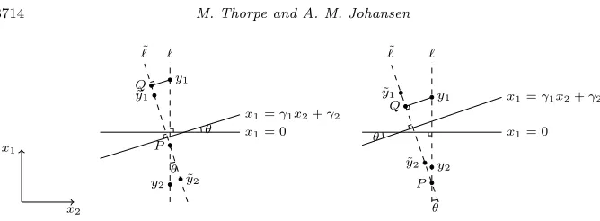
Let be the ray throughy1 andy2 and ˜be the ray through ˜y1 and ˜y2. Let
P be the point of intersection between and ˜. The point P exists if and only if the lines and ˜are not parallel. The lines and ˜ are parallel if and only if
θ= 0, trivially any choice ofθ∗ ≥0 will bound this case. Therefore we assume that θ >0 and therefore the pointP exists.
One can easily show that y˜1P y1 = θ (the angle between the lines ˜y1P and
P y1 is θ). There are two possibilities, either (1)P is between y1 and y2 or (2) it isn’t.
In the second case we assume that|y2−P|<|y1−P|and therefore|y1−P|>
δ. Let Q be the closest point on ˜ to y1 (see Figure 2). So, P, y1, Q form a triangle with P Qy1 = π2, QP y1 = θ and |Q−y1| ≤ |y1−y˜1| ≤ Cr. Hence sinθ=||Qy1−−y1P|| ≤ Crδ .
The first case is similar. Assume that|y1−P| ≥ |y2−P|then|y1−P| ≥2δ. Let
Qbe the closest point on ˜toy1then|Q−y1| ≤ |y1−y˜1| ≤CrandQP y1=θ,
y1QP = π2. In particular sinθ=||y1Q−−y1P||≤ 2Crδ . In both cases sinθ≤ 2Crδ which implies
dH(By1,y2, By1,˜ y2˜ )≤dH(∂By1,y2, ∂By1,˜ y2˜ )≤rC+ 4M Cr
δ .
Let
B(t) =y∈Rd : j(t, y) is not uniquely defined
and X(r, t) =
y∈B(0, r−β) : dist(y, B(t))≤ ν
(L∞)k
r+4r1−β δ
. By the
3714
Fig 2. The geometry considered in the proof of Lemma4.3admits two cases: in the first (left)
the intersection ofland˜llies betweeny1 andy2; in the second (right) it does not.
dist(y, B(t))≤rC+4M rδ =ν(L∞)k
r+4r1δ−β
. And therefore ify ∈X(r, t) thenjr(t, y) =j(t, y).
We now partition X(r, t) into 2r−β−1 subsets (where t is the smallest
integer greater than or equal tot) by defining
Bmy1,y2 =
y∈By1,y2 : y−y1+y2
2
∈[(m−1)r, mr]
and
Xm(r, t) =
y∈X(r, t) :∃i, js.t. dist(y, Bμmi(t),μj(t))≤ 2rν(L∞)k(δ+ 2r −β) δ
and dist(y, Bμmi(t),μj(t))≤dist(y, Bμmi(t),μj(t)) for all m=m
.
SoX(r, t)⊂ ∪m2=1r−β−1Xm(r, t) (assumingν(L∞)k ≤r−β). This implies
|y|≤r−β
2y−μj(t,y)(t)−μjr(t,y)(t)
·μj(t,y)(t)−μjr(t,y)(t)
φY(y|t) dy
=
X(r,t)
2y−μj(t,y)(t)−μjr(t,y)(t)
·μj(t,y)(t)−μjr(t,y)(t)
φY(y|t) dy
≤2
2r−β−1
m=1
mr+ν(L∞)k
r+4r 1−β δ
×
Xm(r,t)
|μj(t,y)(t)−μjr(t,y)(t)|φY(y|t) dy.
Now if y ∈ Xm(r, t) then y−μj(t)+μi(t)
2
≥ (m−1)r for some i, j and therefore|y| ≥(m−1)r−Awhereμ(L∞)k≤A. In particular
φY(y|t)≤
c1(m−1−A)α ifm > A+ 1
[image:22.612.164.498.90.213.2]