Developing a model for analysis of the cooling loads of a hybrid electric vehicle by using co simulations of verified submodels

warwick.ac.uk/lib-publications

Shojaei , S., McGordon, Andrew, Robinson, Simon, Marco, James and Jennings, P. A. (Paul A.). (2017) Developing a model for analysis of the cooling loads of a hybrid electric vehicle by using co-simulations of verified submodels. Proceedings of the Institution of Mechanical Engineers, Part D: Journal of Automobile Engineering . pp. 1-19.

Permanent WRAP URL:

http://wrap.warwick.ac.uk/88892

Copyright and reuse:

The Warwick Research Archive Portal (WRAP) makes this work of researchers of the University of Warwick available open access under the following conditions.

This article is made available under the Creative Commons Attribution-NonCommercial 4.0 (CC BY-NC 4.0) license and may be reused according to the conditions of the license. For more details see: http://creativecommons.org/licenses/by-nc/4.0/

A note on versions:

The version presented in WRAP is the published version, or, version of record, and may be cited as it appears here.

Original Article

Proc IMechE Part D: J Automobile Engineering

1–19

ÓIMechE 2017

Reprints and permissions:

sagepub.co.uk/journalsPermissions.nav DOI: 10.1177/0954407017707099 journals.sagepub.com/home/pid

Developing a model for analysis of the

cooling loads of a hybrid electric

vehicle by using co-simulations of

verified submodels

Sina Shojaei

, Andrew McGordon

, Simon Robinson

, James Marco

and

Paul Jennings

Abstract

The requirement for including the air-conditioning and the battery-cooling loads within the energy efficiency analyses of a hybrid electric vehicle is widely recognized and has promoted system-level simulations and integrated modelling, esca-lating the challenge of balancing the accuracy and the speed of simulations. In this paper, a hybrid electric vehicle model is created through co-simulation of the passenger cabin, the air conditioning, the battery cooling, and the powertrai. Calibration and verification of the submodels help determine their accuracy in representing the target vehicle and achieve a balance between the model fidelity and the simulation speed. The result is a model which has a higher accuracy and a higher speed than those of similar models developed previously and which provides a reliable tool for a thorough investigation of the cooling loads for different ambient conditions and different duty cycles.

Keywords

Vehicle simulations, system-level simulations, co-simulations, hybrid electric vehicle model, energy efficiency of a hybrid electric vehicle, cooling load

Date received: 1 July 2016; accepted: 10 March 2017

Introduction

The energy efficiencie of electric vehicles (EVs) and hybrid electric vehicle (HEVs) are arguably the most critical contributor to their acceptability in today’s mar-ket. As a result, a significant amount of the research on EVs and HEVs has been motivated by the prospects of a higher energy efficiency. Simulation-based optimisa-tion and model-based optimisaoptimisa-tion have been key parts of the research, leading to the creation of various simu-lation tools, such as PSAT,1Autonomie,2ADVISOR3 and WARPSTAR.4 The majority of these tools are based on MATLAB/Simulink and are traditionally centred on the low-fidelity models of the powertrain subsystem, and crude representations of the energy storage, the power electronics and the auxiliary subsys-tems. Nonetheless, they fit the purpose and have been widely used in driving-cycle calculations, component sizing and energy management optimisation. The need for considering real-world conditions in the calculations has encouraged system-level simulations of EVs and HEVs, by integration of higher-fidelity models of

mechanical,5,6electrical7,8and thermal9components or subsystems of the vehicle. Developing high-accuracy models is far more practical in specialised tools than it is in MATLAB/Simulink. Therefore, co-simulation methods are becoming increasingly popular in system-level simulations.10–12The compromise between higher fidelity but slower models and lower fidelity but faster models still remains and should be addressed according to the specific application of the model and verification against the experimental data.

Of the auxiliary subsystems on HEVs, the electric air conditioning is the most energy demanding and can have a significant impact on the energy efficiency and the performance of the vehicle.13–16The largest load on the electric air conditioning is the thermal load of the

1_{WMG, University of Warwick, UK} 2_{Jaguar Land Rover, UK}

Corresponding author:

passenger cabin,17but the refrigeration circuit also pro-vides cooling power to the traction battery18 and this further increases the power demand of the electric air conditioning. As vehicle batteries become more power-ful, their cooling load becomes more comparable with that of the cabin.18–20The impact of the cooling load of the cabin and the battery on the energy efficiency can be mitigated in various ways,21–23but the first step is to quantify the loads and their impact accurately, either by vehicle tests or, much more practically, by a vehicle-level model. This model should represent both the total the instantaneous cooling loads with sufficient accuracy and still fit the requirement of drive cycle simulations, i.e. flexibility and high speed. Determining the appro-priate model fidelity for this purpose has been studied by various researchers.24–28The present work is focused on developing a representative model of a chosen vehi-cle that can support calculation of hot ambient cooling loads within drive cycle energy efficiency simulations. Such applications allow little compromise on the simu-lation speed owing to their time length. However, based on practical considerations, making use of existing tool and co-simulation techniques is preferable. The approach chosen here is to model the electric air-conditioning subsystem of the target vehicle using the AirConditioning Library of Dymola.29–31 Models of the passenger cabin and the battery-cooling subsystems are also required. These are developed using the open-source Modelica fluid library and are integrated with the electric air-conditioning subsystem model (submo-del). The powertrain of the vehicle, is modelled in WARPSTAR, which is based in MATLAB/Simulink. To ensure that the model is representative of the target vehicle, rigorous calibration and experimental verifica-tion are carried out at the subsystem level. The vehicle model is then constructed from verified submodels which are co-simulated in Simulink with the help of the Functional Mock-up Interface (FMI) standard.32 Subsystem-level and vehicle-level verifications prove that the model is sufficiently accurate and the simula-tion speed is sufficiently fast; therefore, the vehicle model is suitable for the intended applications. In fact, as discussed, the achieved levels of accuracy and simu-lation speed are better than or at least comparable with similar models proposed previously in literature.

The main contribution of this paper is that it intro-duces a new tool for system-level simulations of hybrid vehicles, while outlining the achieved level of accu-racy and the required modelling effort across a range of subsystems. The paper is organised in the following order. The next section introduces the target vehicle and describes the details of the relevant subsystems. The sunbsequent sections explain the submodels and the corresponding verification approach. Then, the model integration and co-simulation process as well as verification of the vehicle-level energy efficiency calculations are outlined. Finally, the scope of the follow-on work and a summary of the current research results are presented.

The target vehicle

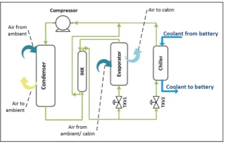
A simplified illustration of the subsystems of the target vehicle is given in Figure 1. This vehicle has an all-wheel-drive parallel hybrid electric powertrain in which a 140 kW diesel engine is coupled to the driveline via a clutch, and a 35 kW electric machine is integrated within the transmission pre-gearbox. The battery pack has 72 cylindrical cells, each with 6.7 A h capacity, which are organised in six modules. The electrical architecture of the pack is 72S1P (72 cells in series).

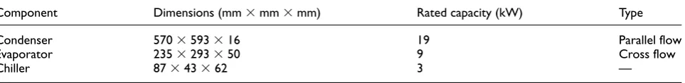
Other subsystems of the vehicle which are of interest are the battery cooling, the electric air conditioning and the passenger cabin. As seen in Figure 1, the battery-cooling circuit includes a pump, an expansion tank and a cooling pipe and is integrated into the refrigeration circuit of the electric air-conditioning subsystem using a refrigerant–coolant heat exchanger (a chiller). The electric air-conditioning subsystem is composed of a refrigeration circuit and air-handling units. The refrig-eration circuit, seen in Figure 1, is composed of a 33 cm3constant-displacement variable-speed electric com-pressor, two air–refrigerant heat exchangers (an eva-porator core and an integrated condenser–subcooler core), an internal refrigerant–refrigerant heat exchanger (IHX), as well as the chiller. The dimensions and the power ratings of the heat exchanger cores are given in Table 1. Two thermostatic expansion valves (TXVs) with integrated shut-off regulate the superheat and the allocation of cooling power to the evaporator and the chiller.

The passenger cabin in this vehicle (not shown in Figure 1) is approximately 2900 mm long and 1700 mm wide, with a shell made of 4.2 m2of glass (i.e. the wind-screen, side windows, rear window, etc.) and 5.2 m2of wall segments (i.e. doors, side posts and the roof). A model is developed for each of the above vehicle sub-systems, and the modelling and verification processes are detailed in the following sections.

The cabin subsystem

Vehicle cabin models are often developed and used for a variety of purposes, such as calculating the thermal loads,33–35 designing the ventilation systems36,37 and understanding the localised thermal conditions experi-enced by passengers;38–41 therefore, such models have various degrees of fidelity and complexity. When the primary aim is to calculate the overall thermal condi-tions of the cabin, lengthy simulacondi-tions can be avoided by using lumped-parameter models which neglect the spatial distribution of temperature and the irregularity of materials within the cabin. The cabin model devel-oped in the current work is based on this approach.

Modelling the cabin

of the shell to calculate the solar heat gain,35,42,43 we assume the significantly simpler geometry in Figure 2, in which the glass and walls forming the cabin shell are modelled as lumped horizontal blocks with areas equal to the total area of glass or wall segments in the cabin shell, and their material properties and temperatures are averaged around the cabin.

The cabin air is represented by a lumped air volume with ideal mixing as proposed previously35,41,42,44 and thermal interactions with the shell and the interiors. In addition to the mass transfer due to ventilation and leakage, the major heat flows that affect the thermal conditions of the vehicle cabin are the solar irradiance, the convection between the shell and the ambient air, the conduction through the shell, the convection between the cabin air and the shell, the convection between the cabin air and the interior, the radiation from the glass and the interior, as well as the heat rejec-tion from passengers. Possible thermal interacrejec-tions with the engine compartment were ignored. It is also assumed that the heat transfer through the floor is lim-ited to that from the battery.

The thermal interactions of the cabin are modelled by using first principles; however, to compensate for the simplifications in the cabin geometry, a number of shape factors are considered which are identified by calibration with the test results. For example, the solar irradiance absorbed by the cabin glass is modelled as

_

Qirr_g,abs=k1_girragSIAg ð1Þ

wherek1irr_g is the shape factor included to account for the variability in the inclination, the curvature and the coatings of the different glass surfaces. A similar model is considered for the irradiance absorbed by the walls. The solar irradiance transmitted through the glass is consequently calculated as

_

Qirr_g,tr=k1_girrtgSIAg ð2Þ

where SI is the solar irradiance. Although a large part of the transmitted component of the solar irradiance is absorbed by the interior, some part of it can continue to exit the cabin environment. Therefore, to approxi-mate the total transmitted irradiance incident that Figure 1. Vehicle subsystems.

TXV2: thermostatic expansion valve 2; eCompressor: electric compressor; IHX: internal refrigerant–refrigerant heat exchanger; TXV1: thermostatic expansion valve 1; EM: electric machine; FDU: front drive unit; RDU: rear drive unit.

Table 1. Heat exchanger specifications.

Component Dimensions (mm3mm3mm) Rated capacity (kW) Type

Condenser 5703593316 19 Parallel flow

Evaporator 2353293350 9 Cross flow

Chiller 87343362 3 —

affects the interior of the cabin, equation (2) is modi-fied by a correction factork2irr

intto give

_

Qirr_int,abs=k2_intirr k2irr_g tg SIAg

ð3Þ

In modelling the interior of the cabin (seats, dashboard, floor and wall carpets, etc.), two separate heat capaci-ties are used. This is to account for the fact that the upper parts of the interior are more exposed to the solar irradiance and can reach significantly higher tempera-tures. The total heat capacity and surface area of the interior was then split between the upper interior and the lower interior.

The heat transfer to the air enclosed in the cabin occurs primarily by convection. In modelling the con-vection between the cabin air and the interior, an aver-age heat transfer coefficient as a function of the interior air flow was used, on the basis of the method proposed by Nielsen et al.33and Zhang et al.36Once the total heat flow to cabin air is calculated, the net internal energy of the cabin air can be calculated from the first law of ther-modynamics on the assumption that air enters and exits the cabin at the same flow rate. The above approach leads to a total of four unknown parameters (the split between the heat capacities of the lower interior and the upper interior, in addition to three shape factors) that should be calibrated to complete the description of the required thermal interactions.

Calibration and verification

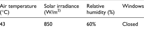
To calibrate the cabin model, the data obtained from pull-down tests and hot-soak tests of the target vehicle in a climatic chamber are used. These tests are part of the standard procedure for evaluating mobile air-conditioning systems.39,45The aim of the pull-down test is to determine the time and the energy required to cool the cabin in hot climate conditions. Typically, the vehi-cle is placed in the climatic chamber for 3 h in the con-ditions given in Table 2. The air-conditioning system is switched on at the maximum power, and the vehicle is

driven over a purpose-built driving cycle. With the assumed conditions, a complete pull-down test of the target vehicle from 60°C to 24°C takes about 4300 s (approximately 1 h 12 min). The aim of the hot-soak test is to determine the maximum temperature experi-enced inside the cabin in an extremely hot climate; thus, the vehicle is placed in the climatic chamber until saturation temperatures are reached. The air tempera-ture and the flow rate, as well as the temperatempera-tures of the shell and the interior, were measured at various points.

The pull-down tests and the hot-soak tests were simu-lated with the ambient conditions, the irradiance, the vehicle speed, the air flow rate and the average vent tem-peratures as the boundary conditions, and the calibra-tion factors were determined through linear regression.

Using the calibrated model, a new pull-down and hot soak test was simulated to verify the model. The measured and simulated cabin air temperatures are compared in Figure 3. It can be seen that very close correlation was achieved, which verifies the suitability of the model for predicting the cabin air temperature in both the cooling scenario and the warming scenario.

Battery-cooling subsystem

As shown in Figure 4, the thermal model of the battery is represented by a heat capacity with thermal interac-tion with the coolant within the cooling pipe and the ambient air. This model does not distinguish between individual cell temperatures.

The heat balance equation of the battery in this model is

Table 2. Climate chamber conditions for pull-down and hot-soak tests.

Air temperature (°C)

Solar irradiance (W/m2)

Relative humidity (%)

Windows

43 850 60% Closed

_

Qamb+Q_cabin+Q_clnt+Q_genCbatt

dTbatt

dt = 0 ð4Þ

in which the heat transfer between the battery and its ambient is given by

_

Qamb=

TambTbatt

Ramb

ð5Þ

the heat transfer between the battery and the interior of the cabin is given by

_

Qcabin=

Tcabin,intTbatt

Rcabin

ð6Þ

and the heat transfer to the coolant is given by

_

Q_clnt=DTln

Rclnt

=m_clntcclntðTclnt,outTclnt,inÞ

ð7Þ

whereDTlnis the logarithmic average of the

tempera-ture between the battery and the coolant along the Figure 4. Layout of the battery-cooling circuit.

Figure 3. Verification of the cabin model against (a) pull-down tests and (b) hot-soak tests: solid curves, test results: dashed curves, simulation results.

length of the cooling pipe. Heat generation within the battery is associated solely with Joule heating46 in this model because other mechanisms of heat generation have little significance for traction batteries and were therefore neglected.47 A list of key parameters of the battery-cooling subsystem is given in Table 3. Verification of the model is carried out in conjunction with the air-conditioning subsystem model in the fol-lowing section.

Air-conditioning subsystem

The air-handling unit of the air-conditioning subsys-tems include the ducts, the vents, the evaporator blower, the condenser (radiator) fan and the air heater. These components were briefly modelled as follows. The air ducts are modelled as frictionless pipes and volumes. The evaporator blower was modelled by implementing the blower characteristic curve as a look-up table. The condenser fan was modelled similarly; however, the total condenser air flow was implemented as a function of the vehicle speed. Also, an ideal air heater model is used to allow reheating of the air stream which exits the evaporator. The rest of this sec-tion covers the model developed for the refrigerasec-tion circuit of the air-conditioning subsystem.

Modelling the refrigeration circuit

The layout of the refrigeration circuit is shown in Figure 5. Various specialised tools29,30,44,48–50 exist for modelling the refrigeration cycles which facilitate the implementation and solution of the equations that describe the thermodynamics of refrigeration. In the present work, the Dymola AirConditioning Library is used, because, despite the fact that it uses a one-dimensional model, it has been shown to represent the steady-state behaviour and transient behaviour of the electric air conditioning with sufficient accuracy. It is beyond the scope of this paper to discuss the refrigera-tion circuit models in detail. A full explanarefrigera-tion can be found in the work by Shojaei et al.,22 Eborn51 and Tummescheit.52 For completeness, a summary of the key attributes pertinent to the problem under investiga-tion are provided for reference, with emphasis on the heat exchangers because of their higher complexity.

Heat exchangers. Basic models of typical heat exchan-gers similar to those used in the refrigeration circuit in Figure 5 are available in the simulation tool. These models are developed based on the (staggered) control volume approach.52,53To customise the existing models for specific components of interest, the constitutive equations (the relationships for the pressure drop and the heat transfer) should be defined through parameter-isation and calibration of the models. This process is detailed below as it is key to achieving an accurate cal-culation of the cooling power available to the cabin and the battery.

For the air–refrigerant heat exchanges (condenser and the evaporator in Figure 5), the air-side heat trans-fer model and the refrigerant-side heat transtrans-fer model are implemented in the general forms

_

Qaw=hawAawðTairTwÞ ð8Þ

and

_

Qwr=hwrAwrðTwTrÞ ð9Þ

respectively, where Aaw and Awr are the heat transfer

areas which can be defined by using the parameterising geometries. In this work, the heat exchanger geometries were accurately defined using a combination of manu-facturer drawings and component measurements. haw

and hwr are functions of the Nusselt number Nu, the

fluid properties and the heat exchanger geometry. Once the geometries are known, the Nusselt number is the only unknown but it can be determined using empirical models and calibration. It was assumed here that the heat flux on the air side of the heat exchanger is the limiting factor. Therefore, for the refrigerant-side heat transfer, the Nusselt number is assumed to be consis-tent with the Dittus–Boelter model54and is given by

Nu= 0:023Re4=5Prn ð10Þ

where the exponent n= 0:3 for heat absorption (eva-porator) and n = 0.4 for heat rejection (condenser). Table 3. Parameters of the battery-cooling subsystem.

Parameter Value

Aamb 0.432 m2

Ramb(0 km/h) 0.9 K/W

Ramb(50 km/h) 0.47 K/W

Rclnt 0.002 K/W

Rcabin 0.06 K/W

cclnt(at 25°C) 3.65 kJ/kg K

Figure 5. Layout of the refrigeration cycle.

IHX: internal refrigerant–refrigerant heat exchanger; TXV1:

For the air-side heat transfer, the Nusselt number was implemented in the general form (see equation (7-1) in the book by Incropera54)

Nu=C1ReC2Prn ð11Þ

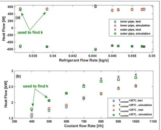
where the coefficientsC1andC2can be calibrated from the experimental data. A set of component characteri-sation data was available for this purpose, in which the cooling power of the heat exchanger is calculated in steady-state conditions. The characterisation procedure is briefly as follows. The refrigerant enters the heat exchanger at a specified pressure and subcooled condi-tions and exists at the pressure set on the heat exchan-ger outlet. A stream of air at a specified temperature and humidity is blown on to the heat exchanger and is cooled or heated as it exits. The mass flow rate of the refrigerant is adjusted to achieve the required superheat for any air flow rate, and the resulting cooling power is measured. Simulating the component models with the boundary conditions of the test, the corresponding Reynolds number and the corresponding Nusselt num-ber can be calculated from the flow conditions and the calculated cooling power. The coefficientsC1andC2in equation (12) were then found by linear regression over a number of the available measurement points and replaced in the models. The models were then verified by comparing the simulations and the test results for the remaining measurement points. As Figure 6 shows,

this process resulted in an accuracy of65%, which is acceptable for the purpose of this model.

The customisation process for the liquid–liquid heat exchangers (the IHX and the battery chiller in Figure 5) is fundamentally similar to that explained above: defining the geometries and calibrating the heat trans-fer models. For the refrigerant side of the chiller the Dittus–Boelter correlation (equation (11)) is used. For the IHX, since the flow is single phase, empirical corre-lations for single-phase flows in circular pipes are used.55To compensate for the geometric incompatibil-ities, a correction factor was assumed, leading to

hcorrected=kh ð12Þ

wherehis the heat transfer coefficient given by empiri-cal correlations and the correction factork= 0.90 was defined by calibration. The resulting heat flows are plotted against the measured data in Figure 7 and show that close correlations were achieved.

A similar calibration and verification approach was employed to define the pressure loss models of the heat exchangers. In the interest of brevity, this process is not discussed further in this work.

Mass flow devices. The compressor and the valves of the circuit of Figure 5 are modelled by simple algebraic equations, since their dynamics are much faster than the average dynamics of refrigeration.56 The Figure 6. Calibration and verification of heat transfer models in the air–refrigerant heat exchangers showing (a) the evaporator power and (b) the condenser power: open circles, test results; open squares, simulation results.

compressor is modelled by describing the ideal mass flow rate of the refrigerant as a function of the rota-tional speed, the displacement and the volumetric effi-ciency, on the assumption of adiabatic compression. The isentropic efficiency map of the compressor is then required to correct the enthalpy values. The efficiency maps were extracted from the component data sheets for the purpose of this work. The electrical efficiency of the compressor was assumed to be 85% independent of its voltage. On the other hand, valve models consist of a volume and a simple pressure loss model with a vari-able flow coefficient. In the TXV models, the flow coef-ficient is controlled by a proportional–integral (PI) controller which mimics the behaviour of the mechani-cal components of the valve.

Steady-state verification of the refrigeration circuit

After the full circuit model in Figure 5 was con-structed from the above components, verification at the circuit level was desirable. Steady-state characteri-sation of the vehicle’s refrigeration circuit was carried out on a test rig at nine test points, and the data set was used to verify the model. The verification results plotted in Figure 8 imply good correlation. The errors in the simulated chiller temperatures and simulated evaporator temperatures in Figure 8(b) and Figure 8(c) respectively are less than 3°C. Also the refrigerant pres-sures on both the high-pressure side and the low-pressure side were predicted with61.5 bar error. These results imply an accuracy which is similar to or better than those given by the models of equivalent fidelity

proposed by Huang et al.,24 Kiss et al.44 and Braun et al.51Transient verification of the model is discussed in the following section.

Transient verification of the refrigeration circuit and

the battery-cooling circuit

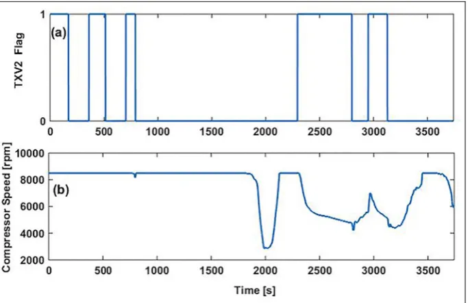
For transient verification of the refrigeration circuit, the vehicle was tested in a climatic chamber at 43 °C. The refrigeration circuit and the battery-cooling circuit were instrumented. Here, as seen in Figure 9, the refrig-eration circuit model and the battery-cooling circuit model are integrated. The battery average temperature, the TXV2 flag, the evaporator inlet air temperature and the compressor velocity are used as inputs. The condenser air flow rate is calculated from the vehicle speed, and the evaporator air flow is known from the fan specifications.

Figure 10 shows the on–off flag of the battery chiller TXV (TXV 2) and the compressor speed, which are the control signals and have the highest transients com-pared with the other inputs to the models.

In Figure 11 the simulated temperatures and the measured temperatures of the average evaporator air-off, the coolant at the battery inlet and the average condenser air-off are compared. As the figure shows, the model represents all the major system dynamics with an absolute error of less than 4°C. A possible rea-son behind this inaccuracy is that the presence of lubri-cation oil in the refrigeration circuit and its potential impact on the heat transfer properties of the refrigerant are neglected.

Figure 12(a) and Figure 12(b) show that the model was able to calculate the refrigerant pressure at the suc-tion port and the discharge port of the compressor,

leading to a reasonably accurate calculation of the compressor power (Figure 12(c)). The results achieved here are more accurate than those reported by Nielsen Figure 8. Verification of the refrigeration circuit model against the test rig measurement for (a) the coolant temperature at the chiller outlet, (b) the average evaporator air temperature, (c) the suction pressure and (d) the discharge pressure: black bars, test results: light bars, simulation results. For test points 1 to 3, both the evaporator and the chiller are in the circuit; for test points 4 to 6, only the evaporator is present in the circuit (the chiller is isolated); for test points 7 to 9, only the chiller is present in the circuit (the evaporator is isolated).

Temp.: temperature; Evap.: evaporator.

Figure 9. Integrated refrigeration and coolant circuits as assumed for transient verification.

IHX: internal refrigerant–refrigerant heat exchanger; TXV1: thermostatic expansion valve 1; TXV2: thermostatic expansion valve 2.

et al.33 and Orofino et al.57 and are comparable with the results reported by Ling et al.;28therefore, it can be concluded that the air-conditioning submodel and the battery-cooling submodel are appropriate for the intended application.

The powertrain subsystem

The powertrain model was developed in WARPSTAR on the basis of the longitudinal dynamics of the vehicle with the general form

Figure 10. Control signals used as the inputs to the model in the verification process: (a) flag signal of TXV 2; (b) the compressor velocity.

TXV2: thermostatic expansion valve 2; Comp. Vel.: compressor velocity; rpm: r/min.

Figure 11. Verification results of the integrated refrigeration and battery-cooling circuit model against the transient vehicle data for (a) the average evaporator (air) temperature, (b) the coolant temperature and (c) the condenser temperature: solid curves, test results; dashed curves, simulation results.

hb

R teng

hbv R ,u

+tem

hbv

R

FRRFA

= M+Ieq

R2

dv dt

ð13Þ

Details of the equations have been given in the rele-vant documents and literature.4 Once the model was parameterised for the target vehicle, experimental verifi-cation was required. The vehicle was tested on a chassis dynamometer, and its controller area network signals were logged. Details of this test were consistent with the European Union test procedures.58 Table 4 lists the details most relevant to this work.

The dynamometer test enables verifications at both component level and subsystem level. The intention here is to outline the process and to illustrate the level of accuracy which the component models deliver.

Therefore, the discussions are limited to verification of the engine and the complete powertrain model.

Component-level verification

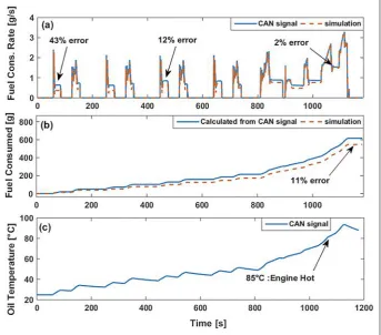
To verify the engine model, it was simulated with logged brake torque and angular velocity signals as the inputs. The simulated and logged fuel consumption val-ues were then compared, as in Figure 13.

The simulated fuel flow rate in the above figure is consistent with the inputs. However, an offset between the simulated fuel flow rate signals and the logged fuel flow rate signals is seen (which is more obvious over cruise periods) and led to 11% underestimation of the total consumed fuel over the driving cycle. This error is due to the low fidelity since only hot engine fuel maps at 90°C and high-temperature driveline efficiency maps Figure 12. Verification results of the integrated refrigeration and battery-cooling circuit model against the transient vehicle data for (a) the compressor suction pressure, (b) the compressor discharge pressure and (c) the compressor electric power: solid curves, test results; dashed curves, simulation results.

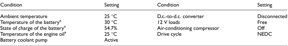
Table 4. Conditions for the powertrain characterisation test.

Condition Setting Condition Setting

Ambient temperature 25°C D.c.-to-d.c. converter Disconnected

Temperature of the batterya 30°C 12 V loads Free

State of charge of the batterya 54.7% Air-conditioning compressor Off

Temperature of the engine oila 25°C Drive cycle NEDC

Battery coolant pump Active

NEDC: New European Driving Cycle. a

Initial values.

were used in the model. According to the test regula-tions, the vehicle starts cold (from 25 °C); thus, the error is large in the beginning but fades away as the components gradually warm up. The issue can be resolved by modelling the thermal behaviour of the engine and driveline components and interpolating between the hot maps and the cold maps at the cost of increased computation but, since the intended applica-tion is simulating hot-climate scenarios, the level of accuracy seen in Figure 13 is considered sufficient.

Subsystem-level verification

Verification of the complete powertrain model can be achieved by simulating it with the logged vehicle speed profile as the input. It is worth mentioning that, since the exact control algorithms of the target vehicle are not used, any comparison between the simulations and the test results at this level are inevitably prone to error but are helpful for understanding the overall perfor-mance of the control rules and for identifying areas for improvement. Figure 14 compares the logged and simulated engine velocities and torques and the logged and simulated electric machine velocities and torques, as well as the battery state-of-charge (SoC) signals. This figure shows an acceptable correlation between the engine velocities and the electric machine velocities, which also indicates that the rule-based controller closely

reconstructed the major operation modes of the vehicle, i.e. low-speed drive in the EV mode, hybrid drive above 24 km/h, engine stop and regeneration, etc. Although some of the discrepancies seen in the engine torques and the electric machine torques are due to noise, the major-ity are driven by the error in the SoC. The logged SoC decreases more rapidly than the model estimates, drop-ping below the lower limit of 50% earlier and shifting the charge event in time, as indicated in Figure 14(d) and Figure 14(e). A closer investigation of the results shows that this error is in fact due to an inaccuracy in the current measurements rather than to a model inaccu-racy. Similar observations prove that simulation results were consistent with the assumed model fidelity and con-trol rules, suggesting that the powertrain model is suit-able for the intended application.

Model integration

The vehicle model was developed by co-simulations of the above submodels in Simulink. For vehicle energy efficiency simulations, it is common to discretise vehicle driving cycles with discretisation steps as large as 1 s. This helps to improve the simulation speed without compromising the accuracy required for these simula-tions. Therefore, the powertrain model should be simu-lated with discrete fixed-step solvers. On the other Figure 13. Engine model verification results for (a) the fuel flow rate, (b) the total fuel consumed against the test results and (c) the variations in the oil temperature: solid curves, test results; dashed curves, simulation results.

hand, the thermal model is better simulated with the variable-step solvers of Dymola which are optimised to handle the non-linear behaviour of the refrigerant and air.59To achieve this, the thermal model was imported to Simulink using the FMI standard which enables Dymola solvers to be embedded in the exported code and to be used to simulate the code within Simulink.60,61Figure 15 shows the layout of the model and highlights the variability in local solvers. As the figure suggests, the thermal model uses two outputs of the powertrain model: first, the vehicle speed which is used to calculate the air flow through the condenser; second, the heat generation within the battery. In turn, the powertrain model receives the battery temperature and compressor power signals from the thermal model.

The controller block in Figure 15 includes the con-trol algorithms of both the powertrain model and the thermal model; the former is described in WARPSTAR documents but the latter can be briefly explained as

follows. The general requirement for cooling the bat-tery is to keep its temperature between 30 °C and 35

°C. The cabin temperature should be maintained between 22°C and 23°C. A state machine is employed that uses the temperature limits to determine the oper-ating state, i.e. the on–off switch of the compressor and the open–close flag of the refrigerant shut-off valves. The velocity of the compressor is controlled via two PI controllers, as seen in Figure 16(a). When the cabin is cooled, the compressor is controlled to maintain the evaporator temperature above 5°C. When only battery cooling is active, the controller maintains the chiller temperature above 10 °C. Also, as shown in Figure 16(b), a third PI controller regulates the air flow from the blower on the basis of the cabin temperature.

Using the model, the vehicle energy consumption is calculated for hot ambient conditions (Tair = 35 °C;

solar irradiance, 800 W/m2) over the New European Driving Cycle (NEDC) and the Worldwide Figure 14. Verification of powertrain model (a) the engine speed and (b) the electric machine speed (c) engine torque, (d) electric machine torque (e) SoC solid curves, test results; dashed curves, simulation results.

eMachine: electric machine; Trq: torque; Spd: speed, SoC: state of charge.

Harmonised Light Vehicles Test Procedure (WLTP) cycle and the results are plotted in Figure 17. Figure 17(a) also shows the energy consumption for the stan-dard 25°C ambient condition (air conditioning off) as the baseline for comparisons. The baseline simulation results over the NEDC show an underestimation of 11% in the fuel consumption compared with the values reported for the vehicle, whereas the error is reduced to

4% for hot ambient conditions. This higher accuracy is expected because of the assumptions made in modelling the engine, since the temperature of the vehicle is closer to that assumed in the model. Figure 17(a) indicates that the cooling loads reduced the fuel economy of the vehicle by about 20%. It can be seen from Figure 17(b) that the model predicts that the cooling loads change the fuel economy over the WLTP cycle from 6.75 l/100 Figure 15. Layout of the system model in Simulink: the black border lines and arrows indicate the submodels and signals simulated using fixed-step MATLAB solvers; the blue border lines and arrows indicate the submodels and signals simulated with variable-step Dymola; the light brown rectangle indicates the controller.

Batt.: battery; SoC: state of charge; Trans.: transmission; Comp.: compressor; Temp.: temperature; Evap.: evaporator; FMI: Functional Mock-up Interface.

km to 8.35 l/100 km. It should be noted that, although reported figures or quotable test data are not available for the WLTP cycle, these results are consistent with the trends reported by Favre et al.62and that, since the WLTP cycle is significantly longer than the NEDC, using hot efficiency maps is more realistic; thus, an error of 4% or even less is expected.

As stated earlier, as well as accuracy, a suitable tool for vehicle-level calculations should have flexibility and a high speed. In terms of flexibility, the model can simulate various ranges of vehicle speed and ambient conditions. The only limitation is the zero flows of refrigerant and air which lead to discontinuities and cannot be handled by the air-conditioning submodel. Therefore, the compressor and blower controllers should include small offsets for which energy flows should be corrected accordingly. As for the simulation speed, some typical simulation times are given in Table 5. These results are achieved on a machine with a Core i7-2600 central processing unit and a 16 GB memory. Table 5 shows that the complete model is significantly slower than the powertrain model alone. Also, simula-tions with hotter ambient condisimula-tions are more time consuming since more events are generated in the model, e.g. because of more frequent opening and clos-ing of the shut-off valves. Nevertheless, these simula-tion times are acceptable as they are considerably shorter than those reported for similar models by Kiss et al.27and Rasmussen.63

Summary and conclusions

In this paper, a vehicle model was developed to enable the air-conditioning and battery-cooling loads to be included in vehicle-level energy efficiency calculations. Subsystem models were developed on the basis of the specifications of a target vehicle and integrated into Simulink using the FMI co-simulation standard. To achieve a representative model, verification against the experimental data from the target vehicle was embedded in the modelling process. The vehicle model developed here fulfils the requirements of the intended application as it is reasonably flexible, produces suffi-ciently accurate results and has an acceptable speed. One drawback of the modelling approach is its depen-dence on the test data. This dependepen-dence can be reduced Figure 17. Vehicle-level energy consumption: (a) the converted energy; (b) the fuel economy.

NEDC: New European Driving Cycle; Eco.: economy; WLTP: Worldwide Harmonized Light Vehicles Test Procedure.

Table 5 Comparison of the simulation times.

Model Simulation scenario Duration (s)

Powertrain only NEDC 19

WLTP 26

Full model NEDC (mild ambient) 286

NEDC (hot ambient) 314

WLTP (mild ambient) 346

WLTP (hot ambient) 431

NEDC: New European Driving Cycle: WLTP: Worldwide Harmonized Light Vehicles Test Procedure.

by using a more physics-oriented approach, e.g.in the case of the cabin. Additionally, this work highlighted the following.

1. When the aim is to obtain the overall conditions of the passenger cabin, a reduced-order model is ade-quate, and model calibrations such as those pro-posed here can help to avoid the burden of modelling the geometric details of the cabin. 2. Calibration of the heat transfer models in the

battery-cooling plate and the heat exchangers were crucial in minimising the modelling and the com-putation effort.

3. A sufficiently accurate representation of the dynamics of the refrigeration circuit and the air-conditioning subsystem can be expected from a one-dimensional model such as those in the AirConditioning Library of Dymola despite vari-ous inherent simplifications. Dymola proved to be a flexible platform for implementing empirical cor-relations which played key roles in achieving a suf-ficiently accurate representation of the thermal processes with a low-order model.

4. This work reaffirmed that a purpose-built model can help to overcome the challenges of system-level simulations, i.e. balancing the accuracy and the speed. Here, subsystem-level verifications helped to determine the fidelity necessary for each submodel early in the modelling process, and awareness of the intended application allowed var-ious simplifications. An example of such simplifi-cations were the temperature-dependent variations in the efficiency of the powertrain which proved to be negligible for the intended application.

The model developed here is appropriate for ana-lysing the energy requirement of air conditioning and battery cooling for hot ambient conditions and repre-sentative duty cycles similar those discussed by Shojaei et al.64These analyses can support the design of alternative thermal management strategies to reduce the impact of the cooling loads on the energy efficiency and performance of the vehicle. Although the correlations achieved above between the simula-tions and the test results are considered sufficient for this purpose, further development of some aspects of the model can enhance confidence in the subsequent analysis. Modelling the effect of the oil circulation in the refrigeration circuit and investigating its impact on the response of the model should be included in this development process. Also, additional investiga-tions of the inaccuracies observed in the battery cur-rent signal that was logged from the controller area network of the vehicle is required to establish a possi-ble requirement for higher fidelity to obtain the underlying reason.

Declaration of conflict of interest

The authors declare that there is no conflict of interest.

Funding

This work was supported by Innovative UK through the Warwick Manufacturing Group Centre High Value Manufacturing Catapult in collaboration with Jaguar Land Rover (EPSRC - EP/I01585X/1).

References

1. Rousseau A, Sharer P, Besnier F. Feasibility of Reusable Vehicle Modeling: Application to Hybrid Vehicles. In: SAE Technical Paper. 2004

2. Halbach S, Sharer P, Pagerit S et al. Model architecture, methods, and interfaces for efficient math-based design and simulation of automotive control systems. SAE paper 2010-01-0241, 2010.

3. Markel T, Brooker A, Hendricks T et al. ADVISOR: a

systems analysis tool for advanced vehicle modeling. J

Power Sources2002; 110: 255–266.

4. Walker A, McGordon A, Hannis G et al. A novel struc-ture for comprehensive HEV powertrain modelling. In: 2006 IEEE vehicle power and propulsion conference, Windsor, Berkshire, UK, 6–8 September 2006, pp. 1–5. New York: IEEE.

5. Gopal RV and Rousseau AP. System analysis using mul-tiple expert tools. SAE paper 2011-01-0754, 2011. 6. Abel A, Blochwitz T and Eichberger A. Functional

mock-up interface in mechatronic gearshift simulation

for commercial vehicles. In: 9th international Modelica

conference, Munich, Germany, 3–5 September 2012, pp. 775–780. Linko¨ping: Modelica Association.

7. Macbain JA, Conover JJ and Brooker AD. Full vehicle simulation for series hybrid vehicles. SAE paper 2003-01-2301, 2003.

8. Johnson V. Battery performance models in ADVISOR.J

Power Sources2002; 110: 321–329.

9. Samhaber C, Wimmer A and Loibner E. Modeling of engine warm-up with integration of vehicle and engine cycle simulation. SAE paper 2001-01-1697, 2001. 10. Puntigam W, Balic J, Almbauer R et al. Transient

co-simulation of comprehensive vehicle models by time dependent coupling. SAE paper 2006-01-1604, 2006. 11. Dvorak D, Thomas B, Rathberger C et al. Thermal

vehicle-concept study using co-simulation for optimizing

driving range. In:2015 IEEE vehicle power and propulsion

conference, Montreal, Quebec, Canada, 19–22 October 2015, pp. 1–6. New York: IEEE.

12. Regner G, Loibner E and Krammer J. Analysis of transi-ent drive cycles using CRUISE-BOOST co-simulation techniques. SAE paper 2002-01-0627, 2002.

13. Samadani E, Fraser R and Fowler M. Evaluation of air conditioning impact on the electric vehicle range and Li-ion battery life. SAE paper 2014-01-1853, 2014.

14. Gao GG. Investigation of climate control power con-sumption in DTE estimation for electric vehicles power usage of climate control. SAE paper 2014-01-0713, 2014. 15. Kambly KR and Bradley TH. Estimating the HVAC

energy consumption of plug-in electric vehicles.J Power

16. Rugh J and Farrington R. Vehicle ancillary load reduc-tion project close-out report. Technical Report NREL/ TP-540-42454, National Renewable Energy Laboratory, Golden, Colorado, USA, 2008.

17. Farrington RB, Anderson R, Blake DM et al. Challenges and potential solutions for reducing climate control loads in conventional and hybrid electric vehicles. Report, National Renewable Energy Laboratory, Golden, Color-ado, USA, 1999.

18. Rugh JA, Pesaran A and Smith K. Electric vehicle battery thermal issues and thermal management techniques. In: SAE alternative refrigerant and system efficiency

sympo-sium, Scottsdale, Arizona, USA, 27–29 September 2012,

pp. 1–40. Warrendale, Pennsylvania: SAE International. 19. Kru¨ger IL, Limperich D and Schmitz G. Energy

con-sumption of battery cooling in hybrid electric vehicles. In: 14th international refrigeration and air conditioning

confer-ence, West Lafayette, Indiana, USA, 16–19 July 2012,

paper 2334, pp. 1–10. West Lafayette, Indiana: Purdue University Press.

20. Neubauer J and Wood E. Thru-life impacts of driver aggression, climate, cabin thermal management, and bat-tery thermal management on batbat-tery electric vehicle util-ity.J Power Sources2014; 259: 262–275.

21. Roscher MA, Leidholdt W and Trepte J. High efficiency

energy management in BEV applications. Int J Electr

Power Energy Systems2012; 37: 126–130.

22. Shojaei S, Robinson S, Chatham C et al. Modelling the electric air conditioning system in a commercially avail-able vehicle for energy management optimisation. SAE paper 2015-01-0331, 2015..

23. Khayyam H and Bab-Hadiashar A. Adaptive intelligent energy management system of plug-in hybrid electric

vehicle.Energy2014; 69: 319–335.

24. Huang D, O¨ker E, Yang S-L et al. A dynamic computer-aided engineering model for automobile climate control sys-tem simulation and application Part I: A/C component simulations and integration. SAE paper 1999-01-1195, 1999. 25. Joudi KA, Mohammed ASK and Aljanabi MK. Experi-mental and computer performance study of an automo-tive air conditioning system with alternaautomo-tive refrigerants. Energy Conversion Managmt2003; 44: 2959–2976. 26. Zhang Q and Canova M. Lumped-parameter modeling

of an automotive air conditioning system for energy

opti-mization and management. In:ASME 2013 dynamic

sys-tems and control conference, Vol 1: aerial vehicles; aerospace control; alternative energy; automotive control systems; battery systems; beams and flexible structures; biologically-inspired control and its applications; bio-medical and bio-mechanical systems; biobio-medical robots and rehab; bipeds and locomotion; control design methods for advanced powertrain systems and components; control of adv. combustion engines, building energy systems, mechanical systems; control, monitoring, and energy har-vesting of vibratory systems, Palo Alto, California, USA,

21–23 October 2013, paper DSCC2013-3835, pp.

V001T04A003-1–V001T04A003-8. New York: ASME. 27. Kiss T and Lustbader J. Comparison of the accuracy and

speed of transient mobile A/C system simulation models. SAE paper 2014-01-0669, 2014.

28. Ling J, Eisele M, Qiao H et al. Transient modeling and

validation of an automotive secondary loop

air-conditioning system. SAE paper 2014-01-0647, 2014.

29. Modelon. Air Conditioning Library, http://www.modelon.-com/products/modelica-libraries/air-conditioning-library/ (2015, accessed 10 December 2016).

30. Tummescheit H, Eborn J and Pro¨lss K. Airconditioning – a Modelica library for dynamic simulation of AC

sys-tems. In:4th international Modelica conference, Hamburg,

Germany, 7–8 March 2005, pp. 185–192. Linko¨ping: Modelica Association.

31. Tummescheit H, Eborn J and Wagner FJ. Development of a Modelica base library for modeling of

thermo-hydraulic systems. In:Modelica workshop, Lund, Sweden,

23–24 October 2000, pp. 41–51. Linko¨ping: Modelica Association.

32. Blochwitz T, Otter M and A˚kesson J. Functional Mockup Interface 2.0: the standard for tool independent

exchange of simulation models. In: 9th international

Modelica conference, Munich, Germany, 3–5 September 2012, pp. 173–184. Linko¨ping: Modelica Association. 33. Nielsen F, Gullman S, Wallin F et al. Simulation of

energy used for vehicle interior climate. SAE paper 2015-01-9116, 2015.

34. Khamsi Y and Petitjean C. Validation results of automo-tive passenger compartment and its air conditioning

sys-tem modeling.Fuel2000; 2013: 7–9.

35. Jha KK, Bhanot V and Ryali V. A simple model for cal-culating vehicle thermal loads. SAE paper 2013-01-0855, 2013.

36. Zhang H, Dai L, Xu G et al. Studies of air-flow and tem-perature fields inside a passenger compartment for improving thermal comfort and saving energy. Part I:

test/numerical model and validation. Appl Thermal

Engng2009; 29: 2022–2027.

37. Nagano H, Miyamoto I and Kohri I. Numerical analysis of energy efficiency of zone control air-conditioning sys-tem for electric vehicle using numerical manikin. SAE paper 2013-01-0237, 2013.

38. Ingersoll JG, Kalman TG, Maxwell LM et al. Automo-bile passenger compartment thermal comfort model – Part I: compartment cool-down/warmup calculations. SAE paper 920266, 1992.

39. Fujita A, Kanemaru J, Nakagawa H et al. Numerical simulation method to predict the thermal environment

inside a car cabin.JSAE Rev2001; 22: 39–47.

40. Ling J, Aute V, Hwang Y et al. A new computational tool for automotive cabin air temperature simulation. SAE paper 2013-01-0868, 2013.

41. Kaynakli O, Pulat E and Kilic M. Thermal comfort

dur-ing heatdur-ing and cooldur-ing periods in an automobile.Heat

Mass Transfer2005; 41: 449–458.

42. Zheng Y, Mark B and Youmans H. A simple method to calculate vehicle heat load. SAE paper 2011-01-0127, 2011.

43. Huang D, O¨ker E, Yang S-L et al. A dynamic computer-aided engineering model for automobile climate control system simulation and application Part II: passenger compartment simulation and applications. SAE paper 1999-01-1196, 1999.

44. Kiss T, Chaney L and Meyer J. A new automotive air

conditioning system simulation tool developed in

MATLAB/Simulink. SAE paper 2013-01-0850, 2013. 45. Rijnders A. Mobile airconditioning test procedure.

Infor-mal Document GRPE-64-23, United Nations Economic Commission for Europe, Geneva, Switzerland, 2012.

46. Pesaran AA. Battery thermal models for hybrid vehicle

simulations.J Power Sources2002; 110: 377–382.

47. Karnik AY, Fuxman A, Bonkoski P et al. Vehicle power-train thermal management system using model predictive control. SAE paper 2016-01-0215, 2016.

48. Casella F, Otter M, Proelss K et al. The Modelica Fluid and Media Library for modeling of incompressible and

compressible thermo-fluid pipe networks. In:5th

interna-tional Modelica conference, Vienna, Austria, 4–5 Septem-ber 2006, pp. 631–640. Linko¨ping: Modelica Association. 49. MAGNA. Kuli software, http://www.kuli-software.com/

KULI.497.0.html (2016, accessed 29 February 2016).

50. National Renewable Energy Laboratory. CoolSim,

http://www.nrel.gov/vehiclesandfuels/vtm_models_tools. html.

51. Braun M, Caesar R, Limperich D et al. Simulation of a vehicle refrigeration cycle with Dymola/Modelica. SAE paper 2005-01-1899, 2005.

52. Eborn J.On model libraries for thermo-hydraulic

applica-tions. Lund Institute of Technology, 2001

53. Tummescheit H. Design and Implementation of

Object-Oriented Model Libraries using Modelica. Lund Institute of Technology, 2002

54. Incropera FP. Fundamentals of heat and mass transfer.

New York: John Wiley, 2011.

55. Gnieleinski V. Heat transfer in pipe flows. In: VDI heat

atlas. Berlin: Springer, 2010, ch G1, pp. 693–700. 56. Rasmussen BP and Alleyne AG. Control-oriented

model-ing of transcritical vapor compression systems.Trabs ASME,

J Dynamic Systems Measmt Control2004; 126: 54–64. 57. Orofino L, Amante F, Mola S et al. An Integrated

approach for air conditioning and electrical system impact on vehicle fuel consumption and performances analysis: DrivEM 1.0. SAE paper 2007-01-0762, 2007. 58. European Commission. Commission Regulation (EC)

No 692/2008 of 18 July 2008 implementing and amending Regulation (EC) No 715/2007 of the European Parlia-ment and of the Council on type-approval of motor vehi-cles with respect to emissions from light passenger and commercial vehicles (Euro 5 and Euro 6) and on access

to vehicle repair and maintenance information.Off J Eur

Union2008; L 199: 1–136.

59. Liu L, Felgner F and Frey G. Comparison of 4 numerical

solvers for stiff and hybrid systems simulation. In:15th

2010 IEEE international conference on emerging technolo-gies and factory automation, Bilbao, Spain, 2010, pp. 1–8. New York: IEEE.

60. Functional mock-up interface, FMI support in Dymola. Ve´lizy-Villacoublay: Dassault Syste`mes AB.

61. Lawrence Livermore National Laboratory.

SUN-DIALS: SUite of Nonlinear and DIfferential/ALge-braic Equation Solvers https://computation.llnl.gov/ projects/sundials (accessed 1 December 2016).

62. Favre C, Bosteels D and May J. Exhaust emissions from European market – available passenger cars evaluated on various drive cycles. SAE paper 2013-24-0154, 2013. 63. Rasmussen BP. Dynamic modeling for vapor

compres-sion systems – Part I: literature review. HVAC&R Res

2012; 18: 934–955.

64. Shojaei S, Robinson S, McGordon A et al. Passengers vs. battery: calculation of cooling requirements in a PHEV. SAE paper 2016-01-0241, 2016.

Appendix 1

Notation

Aaw air-side heat transfer area of the heat

exchanger (air-conditioning subsystem) (m2)

Ag area of glass in the cabin shell (cabin

subsystem) (m2)

Awr refrigerant-side heat transfer area of the

heat exchanger (air-conditioning subsystem) (m2)

cclnt specific heat capacity of the coolant

(battery-cooling subsystem) (kJ/kg K) Cbatt specific heat capacity of the battery

(battery-cooling subsystem) (kJ/K)

haw average air-side heat transfer coefficient

of the heat exchanger (air-conditioning subsystem) (W/m2K)

hwr average refrigerant-side heat transfer

coefficient of the heat exchanger (air-conditioning subsystem) (W/m2K) Ieq equivalent inertia of the vehicle

(powertrain subsystem) (kg m2)

_

mclnt mass flow rate of the coolant

(battery-cooling subsystem) (kg/s) M mass of the vehicle (powertrain

subsystem) (kg) Nu Nusselt number

Pr Prandtl number (air-conditioning subsystem)

_

Qamb heat flow between the battery and the

ambient (battery-cooling subsystem) (W)

_

Qcabin heat flow between the cabin and the

ambient (battery-cooling subsystem) (W)

_

Qclnt heat flow between the battery and the

ambient (battery-cooling subsystem) (W)

_

Qgen internal heat generation of the battery

(battery-cooling subsystem) (W)

_

Qirr_g,abs solar irradiance absorbed by the glass (cabin subsystem) (W)

_

Qirr_g,tr solar irradiance transmitted through the glass (cabin subsystem) (W)

_

Qirr_int,abs solar irradiance absorbed by the interior (cabin subsystem) (W)

Ramb battery–ambient heat transfer resistance

(battery-cooling subsystem) (K/W)

Rcabin battery–cabin heat transfer resistance

(battery-cooling subsystem) (K/W)

Rclnt battery–coolant heat transfer resistance

(battery-cooling subsystem) (K/W) Re Reynolds number (air-conditioning

subsystem)

Tair temperature of the air stream

(air-conditioning subsystem) (K)

Tamb ambient temperature (battery-cooling

subsystem) (K)

Tbatt lumped battery temperature

Tcabin,int temperature of the cabin interior (cabin

subsystem) (K)

Tclnt,in temperature of the coolant at the battery

inlet (battery-cooling subsystem) (K)

Tclnt,out temperature of the coolant at the battery

outlet (battery-cooling subsystem) (K) Tr temperature of the refrigerant in the heat

exchanger (air-conditioning subsystem) Tw temperature of the heat exchanger wall

(air-conditioning subsystem)

ag average absorptivity of the glass (cabin

subsystem)

u throttle opening (powertrain subsystem) (%)

tem torque of the electric machine (powertrain

subsystem) (N m)

teng torque of the engine (powertrain

subsystem) (N m)

tg average transmissivity of the glass (cabin

subsystem)

Abbreviations

EV electric vehicle HEV hybrid electric vehicle

FMI Functional Mock-up Interface IHX internal refrigerant–refrigerant heat

exchanger

NEDC New European Driving Cycle PI proportional–integral

SI solar irradiance (cabin subsystem) (W/m2) SoC state of charge

TXV thermostatic expansion valve

WLTP Worldwide Harmonized Light Vehicles Test Procedure