Diffusion on rapidly varying surfaces

(1)

University of Warwick institutional repository: http://go.warwick.ac.uk/wrap

A Thesis Submitted for the Degree of PhD at the University of Warwick

http://go.warwick.ac.uk/wrap/60735

This thesis is made available online and is protected by original copyright.

Please scroll down to view the document itself.

(2)

Diffusion on Rapidly-Varying Surfaces

by

Andrew Duncan

Thesis

Submitted to the University of Warwick

for the degree of

Doctor of Philosophy

Mathematics Institute

(3)

List of Figures

2.1 Illustration of the scaling for the static, periodic model. . . 14

3.1 Effective diffusion coefficient for an “egg-carton" type surface . . . . 40 3.2 Effective diffusion coefficient for a static, periodic non-symmetric

sur-face. . . 41 3.3 Eigenvalues ofDfor a static, periodic non-symmetric surface . . . . 42 3.4 Effective diffusion coefficient for a surface consisting of periodically

tiled “bumps". . . 43 3.5 Effective diffusion coefficient for a Helfrich elastic membrane in the

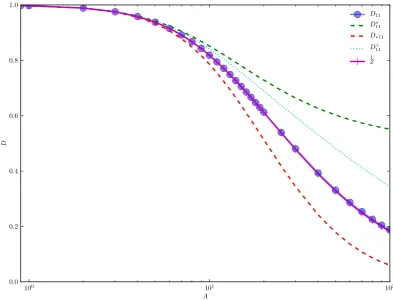
Case I regime. . . 48 3.6 Effective diffusion coefficient for small⇤ for a Helfrich elastic

mem-brane in the Case I regime. . . 49

4.1 Realisation of the “random protrusion surface" . . . 73 4.2 Ergodic average ofDRfor the random protrusion surface forN ! 1. 76 4.3 Convergence of averages ofDRtoDfor the random protrusion surface. 77 4.4 Standard deviation ofDRfor the random protrusion surface. . . 78 4.5 Realisation of the surface generated by stationary Gaussian random

field. . . 80 4.6 Ergodic averages of DR for the Gaussian random field surface for

N _{! 1}. . . 83 4.7 Average values ofDRconverging toDfor the Gaussian random field

surface. . . 84 4.8 Standard deviation ofDRfor the Gaussian random field surface . . . 85

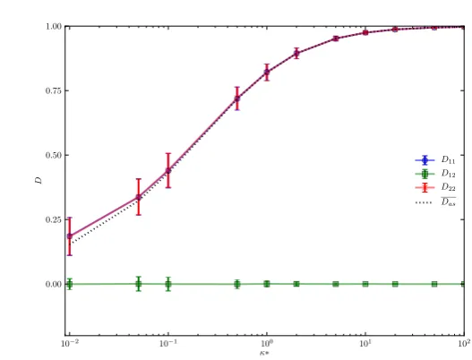
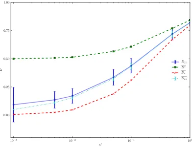
5.1 Effective diffusion coefficient for a Helfrich elastic membrane in the Case II regime. . . 95 5.2 Effective diffusion coefficient for a simple fluctuating surface model

(6)

ACKNOWLEDGMENTS

I would firstly like to thank Professor Andrew Stuart for giving me the opportunity to pursue this research and for the immeasurable amount of guidance, encouragement and support he has provided me with over the last four years. I would also like to express my deepest gratitude to Dr. Grigorios Pavliotis and Professor Charles Elliott for their technical advice, insight and encouragement during this PhD. I am also very grateful to Dr. Björn Stinner whose comments have helped improve the contents of this thesis as well as provided possible future directions of this work. Moreover, I’d also like to thank Professor Peter Kramer from whom I learnt much during his short stay at Warwick.

I would also like to acknowledge the CSC for the computing time onFrancesca

andMinerva.

Thanks are also due to the denizens of room B2.39, past and present, includ-ing, but not limited to, Damon, Dave, Sebastian, Sergios and particularly Tom, who has had to put up with my quirks for the last 4 years. I’d also like to thank Mike, Sebastian and Tom for painstakingly proofreading parts of this thesis, which was no mean feat.

(7)

DECLARATIONS

(8)

ABSTRACT

Lateral diffusion of molecules on surfaces plays a very important role in vari-ous biological processes, including lipid transport across the cell membrane, synap-tic transmission and other phenomena such as exo- and endocytosis, signal trans-duction, chemotaxis and cell growth. In many cases, the surfaces can possess spa-tial inhomogeneities and/or be rapidly changing shape. In this thesis we consider the problem of lateral diffusion on quasi-planar surfaces, which are fluctuating ac-cording to various models. Using homogenisation theory, we show that, under the reasonable assumption of well separated scales, the lateral diffusion process can be well-approximated by a Brownian motion on the plane with constant diffusion co-efficient D. The diffusion coefficient D will depend in a complicated way on the different properties of the surface, such as the average excess surface area, and for biologically motivated models, the bending stress and surface tension.

We consider three classes of surface fluctuation models. The first case we consider is a periodic fluctuation model, where the surface is time-independent pos-sessing rapid, periodic fluctuations. Using classical homogenisation techniques we obtain an expression forDfor a particle diffusing on such a surface and are able to study the various properties ofD. AlthoughDwill not have a closed-form expres-sion in general, we identify a large class of two-dimenexpres-sional surfaces for which the effective diffusion coefficient has an explicit form which depends only on the excess surface area.

The second model we consider is a static, stationary random field model, where the surface is given by a rapidly fluctuating, random field with stationary, ergodic fluctuations. Under appropriate assumptions, we are also able to prove a homogenisation result for lateral diffusion on such a surface and prove results analogous to those for the first model.

Generalising the thermally-excited Helfrich-elastic membrane model, the third case we consider is a fluctuating surface having both rapid spatial and temporal fluc-tuations. The effective diffusion coefficient will depend on the relative scales of the spatial and temporal fluctuations. For different scaling regimes, we prove the exis-tence of a macroscopic limit in each case.

(9)

Chapter 1

INTRODUCTION

Diffusive processes are ubiquitous in physics, chemistry and biology (see [Crank, 1979; Berg, 1993; Van Kampen, 2007]). In biology, diffusion plays a fundamental role in many processes occurring at the cellular and sub-cellular level, and is one of the basic mechanisms for intracellular transport [Bressloff and Newby, 2013]. Diffusion not only occurs within the cell, but can also occur along the cell mem-brane. This lateral diffusion of molecules along the surface of cells also plays a key role in various cellular processes. The lipid molecules and integral membrane pro-teins which constitute the cell membrane themselves undergo lateral diffusion as a result of thermal agitation, [Almeida and Vaz, 1995]. Lateral diffusion of postsy-naptic membrane proteins between synapses is known to play a fundamental part in synaptic transmission, [Borgdorff et al., 2002; Ashby et al., 2006]. Other phenom-ena in which lateral diffusion over biological interfaces is involved include vision [Poo et al., 1974], exo- and endocytosis, signal transduction, chemotaxis and cell growth (see [Sbalzarini et al., 2006] and [Almeida and Vaz, 1995]).

Experimental techniques such as single particle tracking, [Saxton and Jacobson, 1997], fluorescence recovery after photobleaching (FRAP), [Axelrod et al., 1976] and nuclear magnetic resonance (NMR), [Lindblom and Orädd, 1994] have made it possible to accurately measure displacement in a laboratory fixed plane of molecules diffusing laterally on the surface, and thus to measure the macroscopic diffusion co-efficientDof the trajectory of the diffusive process, projected into the plane.

Biological interfaces, however, are not typically flat. Indeed, many membranes will exhibit a non-zero curvature which is induced by the natural spontaneous curvature of the constituent lipids [Seifert, 1997]. They may also be rough, or possess some spatial microstructure. Moreover, the shape of the membrane is changing in time due to thermal fluctuations and possibly also non-thermal fluctuations induced by active membrane proteins on the surface [Gov, 2004].

(10)

the diffusing protein on the surface itself. The relationship between the molecular diffusion coefficient and the measured diffusion coefficient has been widely studied for different types of biomembrane. Previous work such as [Gustafsson and Halle, 1997; Naji and Brown, 2007; Halle and Gustafsson, 1997] and [Sbalzarini et al., 2006] focus on the problem of lateral diffusion of a particle on a static membrane. Various estimates forDin terms of the surface fluctuation were derived, most no-tably the effective medium approximation and area scaling approximation [Gustafs-son and Halle, 1997] and [Sokolov, 1987], and [Naji and Brown, 2007]. Other studies such as [Reister and Seifert, 2007; Reister-Gottfried et al., 2007, 2010] have focussed on the problem of diffusion on a thermally excited biomembrane fluctuat-ing in a hydrodynamic medium, and derived expressions for the effective diffusion coefficient as a function of surface parameters such as bending rigidity, surface ten-sion and fluid viscosity.

The common factor in these models is the presence of small length and time scales in the resulting evolution equations, which enter due to spatial surface microstruc-ture, or due to rapid temporal fluctuations of the surface or possibly both. The objective of this thesis is to investigate the macroscopic behaviour of a laterally diffusive process on surfaces possessing multiple space and time scales using a sin-gle, unified mathematical approach. By doing so we provide rigorous justification for some existing approximations advocated in the literature, clearly explaining the parametric regimes in which they apply, and we develop a systematic methodology which can be used to study other similar problems. Under the assumption that the slow and fast scales are well-separated it is possible to show that the diffusion pro-cess can be approximated by a constant-coefficient diffusion propro-cess on the plane, independent of the small scale, but which accounts for the macroscopic effects of the fine spatial structure and rapid fluctuations. We use the classical methods of averaging and homogenisation (e.g. [Bensoussan et al., 1978; Pavliotis and Stu-art, 2008]) and derive explicit expressions for the coefficients of the macroscopic process in terms of averages with respect to a relevant measure reflecting the rapid fluctuations, and involving solution of the auxiliarycell equationin the case of ho-mogenisation. Although these coefficients will not have a closed form in general, they can be computed numerically, accurately and efficiently without having to sim-ulate effects at the microscopic level, and they are amenable to analysis in various parameter regimes of interest.

(11)

a Helfrich membrane undergoing thermal fluctuations. They identify two limiting regimes: the diffusive limit (homogenization) of a diffusion on a quenched surface and the annealed limit (averaging) of diffusion on a rapidly fluctuating membrane, based on a formal analysis of the Fokker-Planck equation describing the evolution of the system, using the methodology of [Risken, 1996]. They then use numeri-cal methods to study the dynamics of the intermediate regimes where there is no separation of scales. However, to our knowledge, there are no studies which adopt a rigorous multiscale approach to solving this problem, nor are we aware of any work which unifies the study of lateral diffusion on surfaces with both rapid spatial and temporal fluctuations in a single framework. Moreover, we are not aware of any study which makes use of multiscale methods to compute the effective diffusion coefficient directly rather than using direct numerical simulation of the multiscale process, with the exception of [Abdulle and Schwab, 2005] in which the authors describe an HMM (heterogenous multiscale method) scheme for computing the so-lution of an elliptic partial differential equation (PDE) on a static surface possessing fine locally-periodic undulations and rigorously prove convergence of the scheme.

1.1 OVERVIEW OF THE THESIS

We briefly describe the organisation of this thesis and summarise the contents of each chapter.

Chapter 2 provides an overview of the basic results regarding lateral diffusion on quasi-planar surfaces, both from a stochastic differential equation (SDE) perspective and a PDE perspective. We also describe a widely-used two-dimensional continuum model for modelling a fluctuating membrane, based on the Canham-Helfrich elastic free energy [Canham, 1970; Helfrich et al., 1973]. After non-dimensionalisation of the coupled equation describing the particle-membrane evolution, we identify a natural scaling of the problem, and show that for some choices of parameters, the system is well described by its annealed disorder limit (see Naji and Brown [2007]; Reister and Seifert [2007]). We also introduce three simple models which will be studied in the subsequent chapters.

In Chapter 3 we consider the simplest model for surface fluctuations, namely where the surface is described by a static, periodic function. We identify a natural scaling for the surface in terms of a small-scale parameter✏. Using classical homogenisa-tion techniques, we derive a limiting equahomogenisa-tion for a diffusion on this surface in the limit of vanishing✏, and use various standard results from classical homogenisation theory to obtain expressions or approximations forD.

(12)

In Chapter 5 we consider a simple model for a time-dependent, spatially fluctuating surface possessing rapid spatial and temporal fluctuations, which is a generalisation of the fluctuating Helfrich elastic membrane model. The limiting behaviour will depend on the relative speed between the spatial and temporal fluctuations, which is determined by two parameters↵ and , respectively. We consider four natural choices of ↵ and , and for each case study the effective properties of the corre-sponding limit processes. In this chapter we only provide formal justifications of the homogenisation results, using formal perturbation expansions. So as not to break the flow of this chapter the rigorous justification of these results will be deferred to Appendix A.

In Chapter 6, for the particular case of the thermally excited Helfrich elastic mem-brane model, we consider the remaining possible choices of↵and and enumerate all the possible distinguished limits of this model.

In Appendix A we prove the homogenisation results for the four scaling limits de-scribed in Chapter 5 using probabilistic methods.

(13)

Chapter 2

BACKGROUND

2.1 LATERAL DIFFUSION ON FLUCTUATING SURFACES

In this section we describe the formulation of Brownian motion moving on a time-dependent surface embedded in_Rd+1_{. We are primarily interested in quasi-planar}

membranes, so we will restrict our attention to surfaces which can be represented in theMonge parametrisation, that is, surfaces which can be expressed as the graph of a sufficiently smooth functionH:_Rd_⇥_[0_,₁₎_!_R_{. Such a surface}_S₍_t₎_{can then} be parametrised over_Rd_by_J _:_Rd_⇥_[0_,₁₎_!_Rd+1 _{given by}

J(x, t) = (x, H(x, t)).

The function H is known as the Monge gauge. Although this choice of paramet-risation restricts the representable surfaces (overhangs, in particular, are prohib-ited), it greatly simplifies the exposition that follows. In local coordinatesx 2 Rd_, the metric tensor ofS(t)induced fromRd+1_{, can be written as}

G(x, t) =I+_rH(x, t)_{⌦ r}H(x, t) (2.1)

and the infinitesimal surface area element is given byp|G|(x, t), where

|G_|(x, t) := det G(x, t) = 1 +_|_rH(x, t)_|2. (2.2)

It is clear that for any unit vectore₂Rd_,

1_e_·G(x, t)e__|G_|(x, t), for allx₂Rd,

so thatG 1 is symmetric, positive definite (though not necessarily uniformly so). GivenF :Rd+1 _!Rsmooth in a neighbourhood ofS(t), the tangential gradient of

F is given in local coordinates by

(14)

Here,P(x, t)projects vectors inRd+1_{onto the tangent space of}_S₍_t₎_{at local}

coordi-natex, that is,

P(x, t) =I ⌫(x, t)⌦⌫(x, t),

where⌫(x, t)is the surface unit normal ofS(t). The tangential divergencerS(t)·is then obtained from the tangential gradient by contraction. The generalisation of the Laplace operator to curved surfaces is the Laplace-Beltrami operator S(t) which is

given by

S(t)F =rS(t)·rS(t)F.

One can show [Deckelnick et al., 2005; Dziuk and Elliott, 2013] that in local coor-dinates, S(t)acts on smooth functionsF 2C2(Rd+1)as follows

S(t)F(J(x, t)) =

1

p

|G|(x, t)r·

p

|G_|(x, t)G 1(x, t)_r(F J) (x, t) ,

forx₂Rd. We thus define the operator_Ltacting on functionsf 2C2(Rd)to be the local coordinate representation of the Laplace Beltrami operator:

Ltf(x, t) =

1

p

|G|(x, t)r·

p

|G_|(x, t)G 1(x, t)_rf(x, t) , forx₂_Rd. (2.3)

It is clear that S(t)F(J(x, t)) = Lt(F J) (x, t),for all x 2 Rd,t 0 and for all F ₂C2(Rd+1). Notice that for a flat surface, for whichH _⌘0, the operator reduces

to the standard Laplace operator on_Rd_.

2.1.1 BROWNIAN MOTION ON AN EVOLVING SURFACE

While the properties of Brownian motion on static surfaces have been widely studied in the applied literature (see [Van Den Berg and Lewis, 1985; Sbalzarini et al., 2006; Almeida and Vaz, 1995; Naji and Brown, 2007]), Brownian motion on time-dependent surfaces has been given less consideration. In [Naji and Brown, 2007] the authors formally derive the over-damped Langevin equation for diffusion on a surface in the Monge gauge as the limit of a random walk constrained to the surface. In [Coulibaly-Pasquier, 2011], the author provides a rigorous definition of Brownian motion on a manifold with a time-dependent metric. As we are working entirely in the Monge gauge we provide the following natural definition of Brownian motion on a fluctuating Monge-gauge surface, which is equivalent to that given in [Coulibaly-Pasquier, 2011] in the Monge-gauge representation.

Definition 2.1.1. Let(⌦,F,P)be a complete probability space endowed with a

right-continuous filtration(_Ft)t 0. LetS(t)be a time-dependent surface, with corresponding

Monge gauge H(x, t), where H(·, t) 2 C2(Rd). Then, an Rd-valued process Xx(t)

defined on⌦⇥[0, T)is called a Brownian motion onS(t)started atXx(0) =x2Rd,

ifX(t)is continuous, adapted, and if for every smooth functionf :Rd_!_R_,

f(Xx(t)) f(x)

Z t

0 Ls

(15)

is a local martingale (see Definition 5.5, [Karatzas and Shreve, 1991]), where_Ls is

the Laplace-Beltrami operator (2.3) in local coordinates on_Rd_.

We note that in the case whereH _⌘0, Definition 2.1.1 reduces to standard

Brownian motion on_Rd_.

LetS(t)be a time-dependent surface with Monge gaugeH(x, t)such that fort 0,

H(·, t)2C2(Rd). DefineXx(t)to be the solution of the following Itô SDE

dXx(t) =F(Xx(t), t)dt+

p

2⌃(Xx(t), t)dB(t), Xx(0) =x,

(2.4)

where

F(x, t) = p 1

|G(x, t)_|rx·

⇣p

|G(x, t)_|G 1(x, t)⌘, (2.5) and

⌃(x, t) =G 1(x, t), (2.6)

and B(_·) is a standard Rd_{-valued Brownian motion. Here} p_⌃₍_{x, t}₎ _{denotes the} unique positive-definite square root of ⌃(x, t). The existence of a unique strong

solution (in the sense of Section 5.2 of [Karatzas and Shreve, 1991] ) depends on the form ofH(x, t), and we will verify that independently for each surface fluctuation

model we consider. For now we assume that there exists a unique strong solution of the SDE (2.4). Then by Itô’s formula (Theorem 3.3, [Karatzas and Shreve, 1991]), for smoothf :Rd_!R:

f(Xx(t)) f(x) =

Z t

0

1

p

|G_|(Xx(s), s)

rx·

⇣p

|G_|(Xx(s), s)G 1(Xx(s), s)

⌘

rxf(Xx(s))ds

+

Z t

0

G 1(Xx(s), s) :rxrxf(Xx(s))ds

+

Z t

0

p

2G 1₍_X

x(s), s)rxf(Xx(s))dB(s)

=

Z t

0 Ls

f(Xx(s))ds+M(t),

where M(t) is a local martingale. It follows that Xx(t) satisfies the conditions of Definition 2.1.1 to be a Brownian motion on the evolving Monge-gauge surfaceS(t).

Independently, we may derive from first principles the evolution equation for the probability density ⇢(z, t) of a particle undergoing Brownian motion on a

time-dependent surface given expressed in the Monge gauge. From this, we can then recover the same SDE (2.4).

(16)

time-dependent surfaceS(t), and suppose that the process possesses a density⇢(t, z)for

z ₂ S(t). Let⇥be an arbitrary bounded region in _Rd _{with smooth boundary, and} letM(t)be the corresponding region on the fluctuating surface, that is,

M(t) =J(⇥, t).

The density⇢(z, t)is conserved on the surfaceS(t)for alltsuch that

Z

S(t)

⇢(z, t)dz = 1, t 0.

Moreover, we expect that ⇢ flows from regions of low concentration on S(t) to

regions of high concentration, that is we expect that the density flows with local Fickian flux D0rS(t)⇢(z, t) whererS(t) is the tangential derivative on the surface

S(t), and whereD0is a scalar diffusivity constant. It follows that⇢(z, t)satisfies the

following equation

@ @t

Z

M(t)

⇢(z, t)dz =D0

Z

@M(t)rS(t)

⇢(z, t)·n(z, t)dz=

Z

M(t)

D0 S(t)⇢(z, t)dz,

where n(z, t) is the conormal exterior vector along the boundary of M(t). See

[Deckelnick et al., 2005] for details. Changing variables fromzto local coordinates xinduces a change of measuredz =p_|G_|(x, t)dxwhere_|G_|is given by (2.2). We can thus rewrite the above equation in local coordinates as

@ @t

Z

⇥

⇢(J(x, t), t)p|G|(x, t)dx

=

Z

⇥

D0rx·

⇣p

|G|(x, t)G 1(x, t)rx(⇢ J) (x, t)

⌘

dx.

As we are only interested in the trajectory of the diffusion process projected onto the plane, we weight the density ⇢ with the surface area element p|G|(x, t) to

compensate for the local changes in area of the surface. To this end, define the densityq :Rd⇥[0,1)!Rby

q(x, t) :=⇢(J(x, t), t)p_|G_|(x, t).

It is straightforward to check thatR_Rdq(x, t)dx= 1for all timet. Substitutingq(x, t) in the previous equation, and noting that ⇥ is arbitrary, we obtain the following pointwise relationship forq onRd:

@

@tq(x, t) =D0rx·

p

|G|(x, t)G 1(x, t)rx pq(x, t)

|G_|(x, t)

!!

=D0L⇤tq(x, t), (2.7)

(17)

2.2 LATERAL DIFFUSION ON A THERMALLY FLUCTUATING

HELFRICH MEMBRANE

In this section we introduce a particular surface fluctuation model which describes at the mesoscopic level the shape of a quasi-planar bilayer membrane undergoing thermal fluctuations in a low Reynolds number hydrodynamic medium, as derived by [Granek, 1997].

Modelling the bilayer membrane as a two dimensional graph over[0, L]2_with

periodic boundary conditions, we assume that the equilibrium configuration of the membrane is described by the bending energy proposed in [Helfrich et al., 1973] and [Canham, 1970]:

Ebending[H] = 1 2

Z

[0,L]2

⇣

_K(x)2+_KG(x)

⌘ p

|G_|(x)dx,

whereG(x) is the metric tensor of the surface with Monge gaugeH(x)in local

co-ordinates. HereK(x)andKG(x)are the mean curvature and Gaussian curvature of S respectively, [Deckelnick et al., 2005]. The two moduliand are the bending modulus and saddle-splay modulus respectively. Since we assume that the surface does not undergo topological changes during its evolution, by the Gauss-Bonnet the-orem, the integral of the Gaussian curvature depends only on the boundary values, and so can be neglected from the energy functional.

The Helfrich Hamiltonian is commonly defined as elastic bending energy plus an additional term to penalise excess surface area

H[H] =

Z

[0,L]2

⇣_

2K

2₍_x_{) +}

2

⌘ p

|G|(x)dx, (2.8)

where is the surface tension.

For small deformations, |rH(x)_| _⌧ 1, we can make the following approximation

for the mean curvature:

K(x) =_r_· _prH(x)

|G_|(x)

!

⇡ H(x), forx₂[0, L]2

and for the local surface element:

p

|G(x)|⇡1 +1

2|rH(z)|

2_, _for_x₂_[0_{, L}_]2

so that the Helfrich free energy can be approximated by

H[H] = 1 2

Z

[0,L]2

( H(x))2+ _|_rH(x)_|2 dx+ L

2

(18)

The constant term is discarded, leaving the form of the Helfrich free energy which will be used throughout this thesis.

Using linear response theory [Van and Carolyn, 2008] we can describe the dynamics of the thermally excited membrane close to equilibrium by

dH(t)

dt =RAH(t) +⇣(t), (2.10)

where

AH(t) = H

H[H(t)] = 

2_H₍_t_{) +} _H₍_t₎_,

and⇣(t), a Gaussian random field white in time and with spatial fluctuations having

mean zero and covariance operator2 (kBT)R, wherekBis the Boltzmann constant, and T is the temperature. This construction ensures that the dynamics in (2.10) satisfies the fluctuation-dissipation relation required to ensure that, formally, the invariant measure is proportional toexp( H/(kBT)).

The operator R controls the characteristic time for Fourier modes of the membrane to return to equilibrium, and will encode the non-local interactions of the membrane through the hydrodynamic medium. Using an approach analogous to [Doi and Edwards, 1988] for polymer dynamics,Ris approximated by

Rf(x) = (⇤⇤f)(x), f 2L2_per([0, L]2)

where⇤ denotes convolution, and ⇤(x)is given by the diagonal part of the Oseen

tensor:

⇤(x) := 1 8⇡ _|x_|, where is the viscosity of the surrounding medium.

As we are only interested in the local displacement of the surface about the plane, we shall assume that surface configurations have mean 0. To this end, denote by

L2_per([0, L]2;R) the space of all square-integrable functions periodic on[0, L]2 with

mean 0 and let eL,k|k2K1 be the standard Fourier basis for L2per([0, L]2;R), indexed by

K1:=Z2\ {(0,0)}.

It is straightforward to check that the invariant measure ofH(t)is given by_N(0,_C)

where

C/kBT

X

k2K1

⇣

|2⇡k|4+ L2|2⇡k|2⌘ 1eL,k(x)⌦eL,k(x).

The operator C 12 satisfies Assumptions 2.9 (i)-(iv) of [Stuart, 2010], so that its

spectra grows commensurately with those of . It follows from Lemma 6.25 of [Stuart, 2010] that the stationary realisations of the random field will be Hölder continuous with exponent ↵ < 1, but not for ↵ = 1. This implies that

(19)

the surface. Indeed,H(x, t)will be almost surely nowhere differentiable so that it is

not possible to consider a laterally diffusive process on a realisation of this random field. To ensure that the realisations of the surface are sufficiently smooth to permit lateral diffusion, we must either add a further regularisation term to the Helfrich Hamiltonian, or introduce an ultraviolet cut-off. Having an ultraviolet cut-off re-duces the SPDE to a finite dimensional system. Since all the previous work (e.g. [Granek, 1997; Lin and Brown, 2004; Reister and Seifert, 2007; Naji and Brown, 2007]) make an ultraviolet cut-off, we adopt the same approach. To this end, we setheL,k,CeL,ki= 0for wave numbersk62K, where

K={k2K1| |k|c},

for some fixed constantc >0and defineK =_|K_|.

SubstitutingH(x, t)of the form

H(x, t) = 1

L2

X

k2K

⌘k(t)eL,k(x), (2.11)

into (2.10) we note that the SPDE diagonalises, and we obtain the following system of SDEs for the Fourier modes⌘k(t):

d⌘k(t) =

_|2⇡k/L_|3+ _|2⇡k/L_|

4 ⌘k(t)dt+

s

kBT L3

2 _|2⇡k_|dWk(t), (2.12)

whereWk(t) = p1₂ W_kr(t) +i W_ki(t) for standard real valued independent Brown-ian motionsW_kr andW_ki. Fork ₆=k0,Wk(t) andWk0(t) are independent except for

thereality constraintthat

W k(t) =Wk⇤(t),

which guarantees thatH(x, t)is real-valued for all time. It is straightforward to see

that each Fourier mode⌘k(t)has invariant measure

µk=N 0,

2kBT L6 _|2⇡k_|4+ L2_|₂_⇡k_|2

!

,

and it is reasonable to assume that⌘k(0)⇠µk.

Consider a particle with macroscopic diffusion coefficientD0, undergoing Brownian

motion on the time-dependent surfaceS(t) with Monge-Gauge H(x, t). Following

Section 2.1.1, the evolution of the particle trajectory is described by the following SDE

dX(t) = p D0

|G_|(X, t)r·

⇣p

|G|(X(t), t)G 1(X(t), t)⌘dt

+p2D0G 1(X(t), t)dB(t),

(20)

whereG(x, t)is the metric tensor corresponding to the Monge GaugeH(x, t), i.e.

G(x, t) =I+_rH(x, t)_{⌦ r}H(x, t),

forH(x, t)given by (2.11).

Letnek(x) =e2⇡ik·x k2K1

o

be the standard periodic fourier basis functions for L2_per([0,1]2). Setting

x=Lx⇤, t=T t⇤, and X(T t⇤) =LX⇤(t⇤),

and choosingT =L2/D0, we can non-dimensionalise (2.13), noting the units of the

parameters in Table 2.1 we obtain the following non-dimensional system of SDEs:

dX⇤(t⇤) = p 1

|G⇤_|₍_X₍_t⇤₎_{, t}⇤₎r·

⇣p

|G⇤_|₍_X⇤₍_t⇤₎_{, t}⇤₎_G⇤ 1₍_X⇤₍_t⇤₎_{, t}⇤₎⌘ _dt⇤

+

q

2G⇤ 1₍_X_⇤₍_t_⇤₎_{, t}_⇤₎_dB₍_t⇤₎_,

d⌘⇤(t⇤) = 1

✏ ⌘

⇤₍_t⇤₎_dt₊

r

2 ⇧

✏ dW(t

⇤₎_,

(2.14)

where

=diag ⇤|2⇡k|

4₊ _⇤_|₂_⇡k_|2 |2⇡k_|

!

k2K

, (2.15)

⇧=diag 1

⇤_|₂_⇡k_|4₊ _⇤ |2⇡k_|2

!

k2K

, (2.16)

and where⇤, ⇤ and✏are dimensionless constants given by

⇤ = 

kBT

, ⇤ = L

2

kBT ,

and

✏= 4 LD0

kBT .

The matrixG(x, t)is the metric tensor of the surface with Monge gauge

H⇤(x, t) =X

k2K

(21)

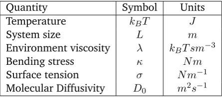
Quantity Symbol Units

Temperature kBT J

System size L m

Environment viscosity kBT sm 3

Bending stress  N m

Surface tension N m 1

[image:21.595.209.432.107.205.2]

Molecular Diffusivity D0 m2s 1

Table 2.1: Model parameters and units

The parameter = ✏ 1 had already been considered in [Naji and Brown, 2007] where it was called thedynamic coupling parameter because it controls the scale separation between the diffusion and the surface fluctuations. As discussed in [Naji and Brown, 2007], for the particular case of band-3 protein diffusion on a human red blood cell, the typical values of parameters result in ✏ _⇡ 0.3, which

suggests that ✏ is an appropriate small-scale parameter. Of course, the value of ✏ will vary greatly for different scenarios.

The limiting behaviour as ✏ ! 0, for the scaling given in equation (2.14) will be

discussed in detail in Section 5.1.2. However, it is a sufficiently simple model to study the limiting behaviour in other scalings, and so we revisit this model in Chap-ter 5 and more exhaustively in ChapChap-ter 6. The main question which we will attempt to answer for each scaling is the dependence of the macroscopic diffusion coefficient on the system parameters⇤, ⇤and the ultraviolet cutoffc(or equivalentlyK).

2.3 MODELS OF RAPIDLY FLUCTUATING SURFACES

In this section we introduce the three main models of fluctuating Monge-gauge sur-faces which will be studied in the thesis. For each model we will derive a system of coupled stochastic differential equations which describe the joint evolution of the particle and the surface. Additionally, we obtain the corresponding Kolmogorov equations for the stochastic system. Although we adopt a primarily probabilistic approach to homogenisation, the PDE formulation is convenient to identify the ho-mogenised equations using formal perturbation expansions. We make use of the PDE approach in Chapters 3 and 5, deferring the rigorous probabilistic proofs to Appendix A.

2.3.1 DIFFUSION ON A STATIC, SPATIALLY PERIODIC SURFACE

(22)

we consider a surfaceS✏_{with Monge gauge given by}

h✏(x) =✏h⇣x ✏

⌘

, (2.17)

where✏is a small scale parameter andhis a sufficiently smooth real-valued function on_Rd_{such that}_h_{and its derivatives are periodic with period}₁_{in every direction.}

We note that as ✏ ! 0, the average surface area is conserved, in the sense that

it remainsO(1)with respect to ✏, which suggests that (2.17) is the natural scaling

for this problem. This is illustrated for the 1D case in Figure 2.1, which plots the surfaceS✏ given byh✏(x)forh(x) = sin(2⇡x)and✏= 1,0.1and0.05. LetZ denote the arc length of the surface over[ 1,1], and consider the projected trajectoryX✏(t)

of a particle undergoing lateral diffusion onS✏_{starting from}₀_{. The escape time of}

X✏(t)from[ 1,1]is equal to the expected escape time of a freeR-valued Brownian

motion from the interval [ Z, Z], which is Z₂2. Taking✏ = _n1 ! 0, the expected

escape time ofX✏ _remains Z2

2 in the limit, which implies that in the limit, the law

ofX✏ _{behaves identically to a free Brownian motion on} _R_{with constant diffusion}

coefficient 1

Z2. We note that any other scaling would result in the surface area going

to 0 or ₁ as ✏ _! 0, which suggests that (2.17) is the only good scaling for this

problem.

-5 -4.18 -1 0 1 4.18 5

= 1

= 0.1

= 0.05

[image:22.595.125.521.392.649.2]

ArclengthZ= 4.188

Figure 2.1: The curveS✏with Monge-Gaugeh✏(x) =✏sin(2⇡x/✏). The three curves

(23)

It is straightforward to see thatS✏ _{has metric tensor}_g✏₍_x_{) =}_g₍_x/✏₎_{, where}

g(x) =I+_rh(x)_{⌦ r}h(x), x₂Td. (2.18)

Consider a particle diffusing along the surfaceS✏and letX✏(t)denote the projection

onto the plane. Following the derivation in Section 2.1.1 withH(x, t) = h✏(x), the

evolution ofX✏₍_t₎_{is given by the following Itô SDE}

dX✏(t) = 1

✏F(X

✏₍_t₎_/✏₎_dt₊p₂_⌃₍_X✏₍_t₎_/✏₎_dB₍_t₎_, (2.19)

whereF(x) and⌃(x) are as in (2.5) and (2.6), but with the dependence ont sup-pressed, i.e.

F(x) = p 1

|g|(x)r·

⇣p

|g_|(x)g 1(x)⌘, and

⌃(x) =g 1(x).

Equivalently, one can consider an observable

u✏(x, t) =E[u(X✏(t)|X✏(0) =x],

where X✏₍_t₎ _{is a Brownian motion on a surface} _S✏ _{given by} _h✏₍_x₎ _{and where} _u ₂

Cb(Rd). The observable u✏(x, t) evolves according to the backward Kolmogorov equation [Friedman, 2006, Chapter 6]:

@u✏(x, t)

@t =L

✏_u✏₍_{x, t}₎_, ₍_{x, t}₎₂_Rd_⇥₍₀_{, T}_]_,

u✏(x, t) =u(x), (x, t)₂Rd_⇥_{0_}.

(2.20)

where

L✏f(x) = _p 1

|g|(x/✏)rx·

⇣p

|g_|(x/✏))g 1(x/✏)_rxf(x)

⌘

. (2.21)

In Chapter 3 we study the asymptotic behaviour of (2.19) and (2.20) in the limit as ✏_! 0. In particular we study how properties of the surface influence the limiting

(24)

2.3.2 DIFFUSION ON A STATIC SURFACE GENERATED BY A SPATIALLY ERGODIC RANDOM FIELD

We can generalise the static, periodic fluctuation model of the previous section con-siderably by replacing the periodic function h(x) in (2.19) with a realisation of a

random fieldh :Rd! Rwith probability measure_P. We assume that the random field has mean0, and is stationary, that is,

EP[h(x)h(y)] =C(x y), x, y2Rd_,

for some non-negative functionC :_Rd_!_R_{. Moreover, we assume that the random} field is ergodic with respect to spatial translations, that is, expectations with respect to P can be replaced by spatial averages (this will be made rigorous in Chapter 4). We also assume that realisations ofh(x)are_P-almost surely bounded and with

bounded derivatives up to order 3.

As in the periodic case, for a fixed realisation h of the random field we consider the surface S✏ with Monge gauge h✏(x) = ✏h(x/✏), where ✏ > 0 is a small scale

parameter. The argument as to why this is the natural scaling for the problem is identical to that in the periodic case.

For a given realisation of h, if we denote by X✏(t) the projected trajectory of a

particle diffusing laterally on the surfaceS✏_{, then the evolution of} _X✏₍_t₎ _{will also}

be described by the Itô SDE (2.19) and the corresponding backward Kolmogorov equation for an observableu✏(x, t)is given by (2.20).

Formulated in this way, the problem is amenable to standard stochastic homogeni-sation methods, such as those in [Papanicolaou et al., 1979; Kipnis and Varadhan, 1986; Komorowski et al., 2012]. In Chapter 4, we use the stochastic homogeni-sation approach to study the behaviour of X✏(t) andu✏(x, t) as✏ ! 0. Given the

assumptions above we can show that in the limit as✏_!0,X✏(t)converges to a free

Brownian motion onRd _{with a constant diffusion coefficient which is determined} by the statistics of the random field (but independent of any particular realisation).

2.3.3 DIFFUSION ON A TIME-DEPENDENT RANDOM SURFACE

The third model we consider is a model for a time-dependent surface possessing both rapid spatial and temporal fluctuations, based on the model discussed in Sec-tion 2.2 for a thermally fluctuating Helfrich membrane. We consider surfaces whose Monge gauge is a time-dependent random fieldH(x, t)such that the following

as-sumptions hold:

1. For eacht 0,H(x, t)is smooth inx;

2. For eacht 0,H(x, t)and its derivatives are periodic inxwith periodLH; 3. For eachx₂_Rd_,_H₍_{x, t}₎_{has characteristic time}_T

(25)

Consider a particle diffusing on a realisation of the surfaceH(x, t)with an isotropic

molecular diffusion coefficientD0. LetX(t)denote the projected trajectory onRd,

and letLand T be the system length and time scales at which the processX(t)is

being observed. We introduce the notation

x=Lx⇤, t=T t⇤, X(T t⇤) =LX⇤(t⇤),

H(x, t) = ˜HH⇤

✓ x LH , t TH ◆ ,

where_H˜ _{is a scaling constant, so that rescaled function} _H⇤ _{has period} ₁ _{in space.}

Define the parameters and⌧ to be

= LH

L and ⌧ =

TH

T , (2.22)

which quantify the scale separation between the diffusion process X(t) and the

spatial and temporal fluctuations respectively.

Substituting these definitions into (2.4) we obtain the following SDE

dX⇤(t⇤)

= 1D0T

L2

1

r

|G⇤_|⇣X⇤(t⇤)_,t⇤

⌧

⌘ry·

0 @

s

|G⇤_|

✓

X⇤₍_t⇤₎

,t⇤ ⌧

◆

G⇤ 1

✓

X⇤(t⇤)

,t⇤ ⌧

◆1 Adt⇤

+

s

2D0T

L2 G⇤ 1

✓

X⇤₍_t⇤₎

,t⇤ ⌧

◆

dB(t⇤),

(2.23)

where

G⇤(y, s)ij = ij+

˜

H LHry

H⇤(y, s)

!

⌦ H˜

LHry

H⇤(y, s)

!

. (2.24)

By choosingT = _DL2₀ andH˜ = LH, we obtain a dimensionless SDE where param-eters and ⌧ measure the spatial and temporal scale separation respectively. To reflect the assumption of rapid spatial and temporal fluctuations we assume that

⌧1and⌧ ⌧1.

Taking the limit of and ⌧ going to zero will give different limits depending on the relationship between these two parameters. To this end, we assume that both⌧ and depend on a common parameter✏as follows

(26)

for scaling parameters↵>0and ₂R. By assuming (2.25), dropping all the stars

and making the dependence ofX on✏ explicit, equation (2.23) can be written as follows

dX✏(t) = 1

✏↵

1

r

|G_|⇣X_✏✏↵(t),_✏t

⌘ry·

⇣p

|G|G 1⌘ ✓X

✏₍_t₎

✏↵ , t ✏ ◆ dt + s

2G 1

✓

X✏₍_t₎

✏↵ ,

t ✏

◆

dB(t).

(2.26)

LetKbe a finite index set with K = _|K_|. As a generalisation of the Helfrich

elas-tic fluctuating membrane model of Section 2.2, we assume that the random field H(x, t)can be written asH(x, t) =h(x,⌘(t)), where

h(x,⌘) =X

k2K

⌘k(t)ek(x) =h⌘(t), e(x)i,

where ek 2 C1(Td); these functions can be extended to Rd by periodicity. The stochastic process⌘(t)is anRK-valued Ornstein-Uhlenbeck (OU) process given by

d⌘(t) = ⌘(t)dt+p2 ⇧dW(t), (2.27)

whereW(_·)is a standard _RK_{-valued Brownian motion. The matrices} _and_⇧ _are symmetric, positive definite. For simplicity, we shall assume that and⇧commute. This is to ensure that the OU process relaxes to equilibrium distribution defined by

N(0,⇧). This theory could be similarly developed without this assumption, but care

must be taken to identify the correct invariant distribution. While this assumption is strong, it is sufficient for the models considered in this paper, and can be relaxed relatively easily.

Substituting this definition ofH(x, t)into (2.23), the evolution of the system can be

described by the joint process(X✏₍_t₎_,_⌘✏₍_t₎₎_{is the solution of the following Itô SDE:}

dX✏(t) = 1

✏↵F

✓

X✏(t)

✏↵ ,⌘ ✏₍_t₎

◆

dt+

s

2⌃

✓

X✏₍_t₎

✏↵ ,⌘✏(t)

◆

dB(t),

d⌘✏(t) = 1

✏ ⌘

✏₍_t₎_dt₊

r

2 ⇧

✏ dW(t)

(2.28)

whereF :Td_⇥_RK _!_Rd_{is given by}

F(x,⌘) := p 1

|g|(x,⌘)r·

⇣p

(27)

⌃:Td_⇥_RK _!_R2⇥2 sym is

⌃(x,⌘) :=g 1(x,⌘), (2.30)

andg(x,⌘) :=I+rh(x,⌘)⌦rh(x,⌘). Since and⇧commute, it is straightforward to check that the OU process⌘✏(t)is ergodic, with unique invariant measure given

by

µ⌘ =N(0,⇧), (2.31)

with measure

⇢⌘(⌘) / exp

✓

⌘·⇧ 1⌘

2

◆

.

For simplicity we will assume that⌘(0) is distributed according to ⇢⌘, so that the

random field is started in stationarity.

Equivalently, one may consider the backward Kolmogorov equation corresponding to (2.28) for the evolution of an observableu✏₍_x,_{⌘, t}₎_:

@u✏(x,⌘, t)

@t =L

✏_u✏₍_x,_{⌘, t}₎_, _for₍_x,_{⌘, t}₎₂_Rd_⇥_RK_⇥₍₀_{, T}₎_,

u✏(x,⌘,0) =u(x,⌘), for(x,⌘)₂Rd_⇥RK.

(2.32)

The infinitesimal generatorL✏can be written as

L✏f(x,⌘) =L✏1f(x,⌘) +L✏2f(x,⌘).

The operator

L✏1f(x) :=

1

p

|g_|(x/✏↵_,_⌘₎rx·

⇣p

|g|(x/✏↵_,_⌘₎_g 1₍_x/✏↵_,_⌘₎_r

xf(x)

⌘

,

encodes the effect of the rapid spatial fluctuations, while

L✏2f(⌘) :=

1

✏ ⌘·r⌘+ ⇧:r⌘r⌘f ,

describes the rapid temporal fluctuations.

The following proposition establishes the well-posedness of equation (2.28) for the joint process(X✏₍_t₎_,_⌘✏₍_t₎₎_.

Proposition 2.3.1. LetX0 and⌘0be random variables, independent ofB(·)andW(·)

such that_E[X0]2 <1andE[⌘]2 <1. Then the system of SDEs (2.28) has a unique

strong solution (X✏(t),⌘✏(t)) satisfying X(0) = X0 and ⌘(0) = ⌘0. Moreover, the

solution(X✏(t),⌘✏(t))₂C([0, T];Rd_⇥RK)is a Markov diffusion process.

Proof. Without loss of generality we consider only ✏ = 1. We apply the results of

Sections 3.2 - 3.4 of [Friedman, 2006]. First we note that the drift and diffusion terms of(2.28)are smooth inX✏_and_{⌘, and so are locally Lipschitz. What remains}

(28)

diffusion terms are clearly bounded since g 1₍_x,_⌘₎

2  1, where | · |2 denotes the

induced matrix 2-norm. We now consider the drift term F(x,⌘) given by (2.29).

Expanding, we have that

|F(x,⌘)| g

1₍_x,_⌘₎_r

x

⇣p

|g|(x,⌘)⌘

p

|g_|(x,⌘) + rx·g

1₍_x,_⌘₎ _, _(2.33)

where forv₂Rd,_|v_|denotes the Euclidean norm inRd. The first term satisfies

g 1(x,⌘)rx

⇣p

|g|(x,⌘)⌘

p

|g_|(x,⌘)  rx

⇣p

|g|(x,⌘)⌘

 |(rpxrxh)rxh|

|g|(x,⌘)

|rxrxh|2

CK|⌘|,

(2.34)

for some positive constantC, where we used (2.2) in the third inequality, and the fact thath(x,⌘) =⌘_·e(x), the componentse(x)and all their derivatives are bounded

to obtain the final inequality. Similarly,

rx·g 1(x,⌘) = 2

⇣

g 1(x,⌘) :_rxrxh(x,⌘)

⌘ ⇣

g 1(x,⌘)_rxh(x,⌘)

⌘

.

Noting that

g 1(x,⌘)rxh(x,⌘) = 1

|g_|(x,⌘)rxh(x,⌘),

it follows that

rx·g 1(x,⌘) 2 g 1

F|rxrxh(x,⌘)|F C

0_K_|_⌘_|_, _(2.35)

for some constantC0 >0, where_|·|_F denotes the Frobenius matrix norm. Together,

(2.34) and (2.35) along with the linearity of ⌘show that

✓

F(x,⌘)

⌘

◆

C00K_|⌘_|,

for some constant C00 independent of x and ⌘. The conclusion of the lemma now follows by Theorems 2.2, 3.6 and 4.2 of [Friedman, 2006].

As before, we wish to study the behaviour ofX✏(t) and it’s corresponding

(29)

that the limiting behaviour will vary for different values of↵ and . In Chapter 5 we will study the scaling limits of (2.28) for the following four scaling regimes.

Case I:↵= 1and = ₁

In this regime the temporal fluctuations occur on a timescale slower than the characteristic timescale of the diffusion process, so far the model can be con-sidered to be a diffusion on a stationary realisation of the surface. This situ-ation has been studied in the case of diffusion on a quenched Helfrich elastic membrane in [Naji and Brown, 2007]. This regime is studied as the problem of diffusion on a static surface with rapid spatial oscillations.

Case II:↵= 0and = 1

The microscopic fluctuations are contributed entirely by the temporal fluctua-tions. The motivating example in this regime is that of diffusion on an Helfrich elastic membrane; this problem has been studied in great detail (see [Naji and Brown, 2007; Gustafsson and Halle, 1997; Reister and Seifert, 2007]).

Case III:↵= 1 and = 1

In this regime we consider lateral diffusion on surfaces possessing both rapid spatial and temporal fluctuations, with the spatial and temporal fluctuations occurring at comparable scales. While this regime has not been studied before, it naturally extends the work covered in [Halle and Gustafsson, 1997; Naji and Brown, 2007; Reister and Seifert, 2007] and helps provide a complete picture. This regime is interesting due to the fact that the limiting diffusion coefficient is in some sense intermediate between that of Case I and Case II.

Case IV:↵ = 1and = 2

In this regime we consider surfaces with both rapid spatial and temporal fluc-tuations but the temporal flucfluc-tuations occur at a faster scale compared to the spatial fluctuations. As in Case III, this regime has not been considered pre-viously, but is studied to provide a complete picture of the possible limiting behaviour.

As we will show in Chapter 5, the limiting behaviour of the process will exhibit dif-ferent behaviour, in particular the effective diffusion will be distinct in each case. For example, if we consider the effective diffusion coefficient for the Helfrich elastic fluc-tuating model, then in the Case II regime, we can show that the (non-dimensional) effective diffusion will converge to 1

2 as the ultraviolet cutoffcconverges to infinity.

On the other hand, in the Case III regime, the effective diffusion coefficient will converge to0.

(30)

H(x, t). As was considered in previous work ([Naji and Brown, 2007] and [Reister

and Seifert, 2007]), studying the properties of the effective diffusion coefficient av-eraged over the surface realisations is more illuminating.

In Case II, the limiting behaviour is determined by the properties of the station-ary distribution of the Ornstein Uhlenbeck process ⌘(t) and deriving the effective

diffusion process can be viewed as an averaging problem (see [Pavliotis and Stuart, 2008]).

In the regimes covered by Case III and Case IV we must consider the interactions between the temporal and spatial fluctuations. In Case III, the spatial fluctuations homogenise the diffusion process “faster" than the temporal fluctuations, and the result is that the effective diffusion coefficient will merely be the effective diffusion coefficient from Case I averaged over the invariant measure of the OU process⌘(t).

SDEs in this scaling limit were considered in [Garnier, 1997].

Deriving a scaling limit in the Case IV regime proves more complicated, due to the lack of an explicit invariant measure for the “fast process". Once the geometric er-godicity of the fast process with respect to a unique invariant measure is established, the approach will be similar to the classical probabilistic homogenisation arguments of [Bensoussan et al., 1978]. Although a limiting equation is established, the lack of an explicit invariant measure, makes it hard to establish bounds on the effective diffusion coefficient.

We have not yet addressed the question of the limiting behaviour ofX✏(t)for other

values of↵and besides those considered in Cases I - IV. The answer to this ques-tion is problem dependent (i.e. dependent on the particular choice ofe(x), and the

(31)

Chapter 3

DIFFUSION ON A STATIC SURFACE

WITH PERIODIC FLUCTUATIONS

In this chapter we study the macroscopic behaviour of particles diffusing laterally on a static surface possessing rapid, periodic fluctuations as described in Section 2.3.1. While this time-independent model is of limited use as a phenomenological model, it benefits from being amenable to classical periodic homogenisation methods and will serve as the basis for the more elaborate models considered in subsequent chap-ters. The problem of diffusion on static, periodically fluctuating surfaces has been previously studied in the literature with varying degrees of rigour. A review of exist-ing work on this problem is given in Section 3.1. While the homogenised equations and the variational bounds for the effective diffusion coefficient have been previ-ously stated (in particular [Halle and Gustafsson, 1997]), to our knowledge these results have never been analysed rigorously as we do here.

We recapitulate the details of Section 2.3.1. Consider the projected trajectoryX✏(t)

of a particle diffusing laterally on the surface with Monge gauge

h✏(x) =✏h⇣x ✏

⌘

, (3.1)

where ✏ > 0 is a small scale parameter and h is a sufficiently smooth real-valued function on_Rd_{which is periodic with periodic derivatives with period}₁_{in all} direc-tions. The particle’s position satisfies the following Itô SDE

dX✏(t) = 1

✏F(X(t)/✏)dt+

p

2⌃(X(t)/✏)dB(t), (S1)

where

F(x) = p 1

|g_|(x)r·

⇣p

|g|(x)g 1(x)⌘, and

(32)

whereg(x)is the metric tensor of the surface with Monge gaugeh(x), i.e.

g(x) =I+_rh(x)_{⌦ r}h(x).

The backward Kolmogorov equation corresponding to (S1), for an observable

u✏(x, t) =_E[u(X✏(t)_|X✏(0) =x],

whereu₂Cb(Rd)is given by:

@u✏(x, t)

@t =L

✏_u✏₍_{x, t}₎_, ₍_{x, t}₎₂_Rd_⇥₍₀_{, T}_]_,

u✏(x, t) =u(x), (x, t)2Rd_⇥_{₀_}_. (P1)

where

L✏f(x) = p 1

|g|(x/✏)rx·

⇣p

|g_|(x/✏)g 1(x/✏)_rxf(x)

⌘

. (3.2)

Our objective is to study the effective behaviour of X✏(t) and u✏(x, t) as ✏ _! 0.

We will show that as✏_!0, the_Rd_{-valued process}_X✏₍_t₎_{will converge weakly to a}

Brownian motion on_Rd_{with constant diffusion coefficient}_D_{which depends on the} surface maph(x). Equivalently, we show thatu✏converges pointwise to the solution u0 _{of the PDE:}

@u0(x, t)

@t =D:rxrxu

0₍_{x, t}₎_, ₍_{x, t}₎₂_Rd_⇥₍₀_{, T}_]_,

u0(x, t) =v(x), (x, t)₂Rd_⇥_{0_}.

(3.3)

Since (S1) (respectively (P1)) is a SDE (resp. PDE) with periodic coefficients, the problem is amenable to classical periodic homogenisation methods, such as those of [Bensoussan et al., 1978; Jikov et al., 1994; Pavliotis and Stuart, 2008]. In Section 3.2 we state the homogenisation result for this model. The result will be justified formally by using perturbation expansions of the PDE in(P1). One can then invoke standard results to obtain a rigorous proof of convergence for both (S1) and (P1).

For d = 1, D depends only on the excess surface area Z (i.e. the average ratio of the surface area of the graph ofhto the area of the base). Indeed, we will show thatD= _Z12. Ford 2, in general, the expression forDdepends of acorrector, the

solution of an auxiliarycell problem, which has no closed-form solution in general. Without making further assumptions on the surface we can obtain at best upper and lower bounds in terms of the functionh which are derived in Section 3.3. In the special case whered= 2andDis isotropic, however, it is possible to obtain a closed form expression for the effective diffusion coefficient, and in Section 3.4, making use of a duality transformation argument we are able to show that D is equal to

1

(33)

is known in the literature as thearea scaling approximation, [Halle and Gustafsson, 1997; Naji and Brown, 2007; King, 2004; Gov, 2006].

The rest of the chapter is organised as follows. In Section 3.5 we identify a nat-ural symmetry condition for the surface maphwhich is sufficient to ensure that D is isotropic, and thus that the area scaling approximation holds. In Section 3.6 we describe a finite element scheme for numerically approximatingD, and in Section 3.7 we use this scheme to perform numerical experiments illustrating the theory of this chapter. Finally, in Section 3.8 we use the results obtained in this chapter to study the effective behaviour of (2.28) in the Case I regime. Although the effective diffusion coefficient will depend on the particular realisation of the surface, we are still able to obtain useful information regarding the average effective diffusion co-efficient (i.e. the effective diffusion coco-efficient averaged over all realisations). We then focus on the specific case of diffusion on a quenched Helfrich elastic surface and study how the limiting behaviour is affected by the model parameters, both analytically and with numerical experiments.

3.1 PREVIOUS WORK

Lateral diffusion on quasi-planar periodic surfaces have been previously studied in the literature, mainly in the context of biological interfaces. The first such work we are aware of is [Aizenbud and Gershon, 1985] where the authors consider the prob-lem of diffusion on a curve possessing rapid periodic fluctuations, with the objective of explaining the slowing down of diffusion of succiny-concanavalin A receptors on the surfaces of adherent mouse fibroblast. The authors derive the effective diffusion coefficient, in this case, given by D = _Z12. In [Halle and Gustafsson, 1997], the

authors study the same problem in two dimensions. By recognizing the problem as diffusion in a potential they use standard results from diffusions in periodic po-tentials to obtain the homogenised diffusion coefficient D in terms of a corrector. Under some implicit symmetry assumptions on the surface, they then derive varia-tional bounds forD. The authors discuss various non-variational bounds for theD, and propose two estimates: the effective medium approximation, given by

Dema= R Z

Td|g|(y)dy I,

and the area scaling approximation, given by

Das=

1

ZI.

(34)

random walks on the surface and estimating the diffusion coefficient using linear regression. The conclusion was thatD _/Z 1.42_{, which is at odds with the results}

presented in here and in [Halle and Gustafsson, 1997].

In [Naji and Brown, 2007], the authors also study the problem of diffusion on a surface given by a realisation of a quenched elastic membrane with periodic fluctu-ations. By performing direct simulation of the Brownian particles over realisations of the surface, the authors estimate the effective diffusion coefficient, averaged over the surface realisations. Based on these numerical estimates, the authors conclude that for static surfaces the area scaling estimate is the most accurate, but do not offer a proof.

More recently, in [Khrabustovskyi, 2009], the author studies the asymptotic be-haviour of the spectra and eigenfunctions of the Laplace-Beltrami operator of a (non-graph) manifold consisting of a bounded two-dimensional domain where small disjoint holes of sizeO(✏), placed periodically with periodO(✏), are removed and

re-placed with “bubbles" -n-dimensional spheres, truncated in a region about the poles. The author then applies the results derived for the spectra to study the asymptotic behaviour of the heat equation on such a surface, and proves convergence of the solution to a diffusion on the plane with effective diffusion coefficient depending on the (possibly slowly varying) radii of the holes.

3.2 HOMOGENIZATION RESULT

For convenience, we introduce the fast processY(t) = X_✏(t) mod Td. We can then express (S1) as the following fast-slow system

dX✏(t) = 1

✏F(Y

✏₍_t₎₎_dt₊p₂_⌃₍_Y✏₍_t₎_dB₍_t₎_,

dY✏(t) = 1

✏2F(Y

✏₍_t₎₎_dt₊

r

2

✏2⌃(Y✏(t))dB(t),

(3.4)

whereX✏(t)2Rd_,_Y✏₍_t₎₂_Td_and_B₍_t₎_{is a standard Brownian motion on}_Rd_{. The} infinitesimal generator of the fast process is theL2(Td)closure of

L0f(y) = p 1

|g_|(y)ry·

⇣p

|g|(y)g 1(y)ryf(y)

⌘

, f 2C2(Td).

It is straightforward to see that L0 is a uniformly elliptic operator with nullspace

containing only constants, that is

N[_L0] =_{1_},

and

(35)

where ⇢(y) =

p |g|(y)

Z , and where Z is the normalisation constant given by Z =

R

Td

p

|g_|(y)dy.

We expect to be able to compute the homogenising effect of the fast process Y✏ on the slow processX✏ _{and thereby compute an effective equation which accounts}

for, but removes explicit reference to, the small scale. Givenv 2C_b2(R2 ⇥Td₎_{, the} observable

v✏(x, y) :=Ehv(X✏(t), Y✏(t)) |X✏(0) =x, Y✏(0) = x

✏

i

satisfies the backward Kolmogorov equation given by:

@v✏(x, y, t)

@t =L

✏_v✏₍_{x, y, t}₎_, ₍_{x, y, t}₎₂_Rd_⇥_Td_⇥₍₀_{, T}_]_, _(3.5)

where

L✏ =_L2+1

✏L1+

1

✏2L0 (3.6)

for

L1v(x, y) :=F(y)_·_rxv(x, y)

+ 2⌃(y) :_rxryv(x, y),

(3.7)

and

L2v(x, y) :=⌃(y) :_rxrxv(x, y). (3.8) Note that the last term in (3.7) reflects the correlation of the noise between the fast and slow processes.

We wish to study the behaviour ofX✏_and_v✏_{in the limit as}_✏_!₀_,

homogenis-ing over the fast variable Y✏ _{to identify a constant coefficient diffusion equation}

which approximates the slow process in some sense. As the corresponding SDE and PDE have periodic coefficients, we can apply results from classical homogenisation theory such as [Bensoussan et al., 1978; Jikov et al., 1994] to prove convergence of X✏andv✏to solutions of limiting equations. We refer to [Pavliotis and Stuart, 2008] for a modern pedagogical treatment of this theory. In this Section we will state the homogenisation result and provide a formal derivation of the limiting equations based on perturbation expansions.

The macroscopic effect of the fast-scale fluctuations is characterised by acorrector

:Td!Rd_{which is the solution of the following}_{cell equation}

L0 (y) = F(y), y₂_Td. (3.9)

Lemma 3.2.1. There exists a unique solution ₂C2₍_Td_;_Rd₎_{such that}

Z

Td

(36)

and which solves (3.9).

Proof. Since _L0 has a compact resolvent, we can apply the Fredholm alternative [Gilbarg and Trudinger, 2001]. This states that the cell equation will have a solution provided the RHS of (3.9) is orthogonal inL2(Td)to the nullspace ofL⇤

0, that is, the

centering conditionholds _Z

Td

F(y)⇢(y)dy=0,

but is trivially true from the definition ofF(y) and ⇢(y). The solution is unique

provided we impose condition (3.10). Finally, 2C2(Td;Rd)follows from standard

elliptic regularity theory.

The following theorem states the homogenisation result for this scaling regime. The proof given is based on formal perturbation expansions which can be used as the basis for a rigorous proof. However, a probabilistic approach based on Theorem 3.1, [Pardoux, 1999] or [Bensoussan et al., 1978] are more succint. In what follows we will adopt the convention that

ry (y) _ij =

@ i

@yj

(y), fori, j ₂1, . . . , d

see Chapter 2 of [Gonzalez and Stuart, 2008].

Theorem 3.2.2. LetT >0, then the processX✏ converges weakly inC([0, T];Rd) to

a Wiener processX0(t)which solves

dX0(t) =p2DdB(t), (3.11)

whereDis the (constant) effective diffusion coefficient given by

D= 1

Z

Td

I+_ry (y) g 1(y) I+ry (y) >

p

|g_|(y)dy, (3.12)

whereZ is the surface area of a single cell of the surface given by

Z =

Z

Td

p

|g|(y)dy. (3.13)

Moreover, if equation (P1) has initial datau(independent of✏)such thatu2C_b2(Rd),

then the solutionu✏ of (P1) converges pointwise to the solutionu0 of (3.3) uniformly

with respect totover[0, T].

Formal justification of Theorem 3.2.2. To derive the homogenised equation in this regime we make the ansatz that the solutionv✏ _{of the backward Kolmogorov}

equa-tion (3.5) is of the form