http://dx.doi.org/10.4236/ajcm.2016.63021
How to cite this paper: Mishra, P.J., Singh, T. and Pattanayak, H. (2016) An Optimal Policy with Quadratic Demand, Three- Parameter Weibull Distribution Deterioration Rate, Shortages and Salvage Value. American Journal of Computational Ma-thematics, 6, 200-211. http://dx.doi.org/10.4236/ajcm.2016.63021
An Optimal Policy with Quadratic Demand,
Three-Parameter Weibull Distribution
Deterioration Rate, Shortages and
Salvage Value
Pandit Jagatananda Mishra1, Trailokyanath Singh2*, Hadibandhu Pattanayak3
1Research Scholar, Ravenshaw University, Cuttack, India
2Department of Mathematics, C. V. Raman College of Engineering, Bhubaneswar, India 3Department of Mathematics, Institute of Mathematics and Applications, Bhubaneswar, India
Received 16 April 2016; accepted 12 July 2016; published 15 July 2016
Copyright © 2016 by authors and Scientific Research Publishing Inc.
This work is licensed under the Creative Commons Attribution International License (CC BY). http://creativecommons.org/licenses/by/4.0/
Abstract
The present paper focuses an optimal policy of an inventory model for deteriorating items with generalized demand rate and deterioration rate. Shortages are allowed and partially backlogged. The salvage value is included into deteriorated units. The main objective of the model is to mi-nimize the total cost by optimizing the value of the shortage point, cycle length and order quantity. A numerical example is carried out to illustrate the model and sensitivity analyses of major para-meters are discussed.
Keywords
EOQ, Quadratic Demand, Salvage Value, Shortage, Three-Parameter Weibull Deterioration Rate
1. Introduction
In the recent three decades, rigorous researches have come to existence on inventory models for deteriorating items. Most of the physical goods deteriorate over time. Food items, fruits, vegetables suffer from depletion by direct spoilage while stored. Highly volatile liquids such as alcohol, gasoline and turpentine undergo physical depletion over time through the process of evaporation. Electronic goods, grains, photographic films and radioactive
substances deteriorate through a gradual loss of potential or utility with the passage of time. So decay or deteri-oration of physical items in stock is a very realistic feature and inventory researchers felt the necessary to use this factor into consideration. Generally, deterioration is defined as the natural process that occurs in most of physical items those lose their characteristic over time. It violates the assumption that goods can be held infi-nitely for future demand. The mathematical modeling on inventory control was started with the work of Harris [1], who studied the classical EOQ (Economic Order Quantity) model with his implicit assumption was the stocked items have infinite shelf lives. Researches in this area were started from fashion goods. Firstly, Whitin [2] studied the deterioration on fashion goods after their valid period. After, Ghare and Schrader [3] were the first two researchers who laid the foundation of modeling inventory system of deteriorating items with help of differential equation. They studied the classical inventory model without shortage considering the constant dete-rioration rate. Shah and Jaiswal [4] and Aggarwal [5] developed an order level inventory models considering the constant deterioration rate. Another class of inventory models was developed on the assumptions of the time dependent deterioration rate. Firstly, Covert and Philip [6] developed an EOQ model for deteriorating items us-ing a two-parameter Weibull distribution deterioration rate. Later, Philip [7] extended their model by consider-ing the three-parameter Weibull distribution deterioration rate. Misra [8] first developed the production lot-size model by using both the constant and the two-parameter Weibull distribution deterioration. The review litera-tures on inventory modeling were given in the articles of Raafat [9], Goyal and Giri [10], Li et al. [11] and Bakker et al. [12].
Besides demand and deterioration rate, other factors like allowing shortages are important for modeling of in-ventory. Shortages usually occur in two cases when the shortage items are totally backlogged and the other case when the items are partially backlogged. In the former case, the customers are not totally willing to accept the items while the latter case customers are only willing to accept the items which can be supplied by the whole sellers in the next period. Various types of inventory models with completely backlogging were discussed by Murdeshwar [13], Goyal et al. [14], Chakrabarti and Chaudhuri [15], Salmeh et al. [16], Zhou and Lau [17] and others.
But, in real life situation, during the shortage period, the willingness of a customer to wait for items declines with the length of the waiting time. Backlogging happens due to the lack of raw materials or work in progress or the demand is uncertain. Chang and Dye [18] were the first who studied the backlogging rate that depends on the length of the waiting time. In the real life situations, for many stocks such as fashionable commodities and high-tech products, the longer the waiting time, the smaller would be the backlogging rate. Being the backlog-ging rate as variable, it depends on the length of waiting time for the next replenishment. Many researchers like Papachristos and Skouri [19], Abad [20], Teng et al. [21], Sana [22], Roy et al. [23] and Singh and Pattnayak [24] studied their models with considering the partial backlogging rate.
In the classical EOQ models, the demand rate of an item was assumed as constant. However, in the real mar-ket situations, the demand rate of any item always acts as a dynamic state. In this context, Silver and Meal [25] first developed the modified EOQ model with varying demand. Many researchers like Donaldson [26], Dave and Patel [27], Giri et al.[28] and others worked in this direction. However, most of the above model mainly based on time-varying demands like linearly or exponential. Considering the quadratic demand as the next rea-listic approach, Ghosh and Chaudhuri [29], Khanra et al. [30] and Singh and Pattnayak [31] developed their in-ventory models for deteriorating items. Singh et al. [32] developed an EOQ model for deteriorating items under permissible delay in payment by considering stock dependent demand.
Other category of inventory models was developed by considering the deterioration rate as the key factor. Ghare and Schrader [3], Shah and Jaiswal [4], Aggrawal [5] and Bhunia and Maiti [33] developed their models considering the deterioration as constant. Researchers like Covert and Philip [6], Mishra [8], Jalan et al. [34], Jain and Kumar [35] and Singh and Pattnayak [36] studied their models taking two-parameter Weibull distribu-tion deterioradistribu-tion. In real life situadistribu-tion, the two-parameter Weibull distribudistribu-tion deterioradistribu-tion may not be useful because some items start deteriorating after a certain period while storing, but not at the initial stage. Generally, when the items are kept in stock, they do not start deteriorating as soon as they are received; instead, deteriora-tion starts after some time. For such items three-parameter Weibull distribudeteriora-tion deterioradeteriora-tion rate is applicable to represent the time to deterioration. The location parameter is used to describe its shelf life. Philip [7], Chakra-barti et al. [37] and Jain and Kumar [38] studied their models considering deterioration rate as three-parameter Weibull distribution to represent the time to deterioration.
to the customers to motivate to buy the deteriorated units. In this context, Jaggi and Aggarwal [39], Mishra and Shah [40] developed their models using salvage value one of costs. Recently, Annadurai [41] studied the inven-tory model for deteriorating items with shortages and salvage value.
In this study, an effort has been made to determine an optimal policy for deteriorating items considering qua-dratic demand, three parameter Weibull distribution deterioration rate and salvage value. Shortages are permit-ted to occur and partially backlogged. Among the different patterns of time varying demands, the most realistic approach is to consider the quadratic demand pattern because it represents both accelerated and retarded growth in demand. Quadratic demand is generally represented by R t
( )
= + +a bt ct2,a>0,b≠0,c≠0. When c=0 and b= =c 0, it represents linear and constant demand rates respectively. In real market situations, deteriora-tion starts after some time when the items are stocked. For such items, the three-parameter Weibull distribudeteriora-tion deterioration can be used to represent the time to deterioration. It is generally represented by( )
(
)
1(
) ( ) (
)
, 0 1 , 0 , 0 1
Z t =αβ t−γ β− α <α β > γ < <γ where α β γ, , and t are called scale parameter, shape parameter, location parameter and time of deterioration respectively. When γ =0 and β =1 &γ =0, it represents the two-parameter Weibull and constant deterioration rate respectively.
2. Assumptions
The following assumptions are taken in developing the model. 1) A single product is considered.
2) Replenishment is instantaneous. 3) The lead time is zero.
4) The demand rate is deterministic and quadratic function of time.
5) The deterioration rate is three-parameter Weibull distribution deterioration.
6) The shortages are permitted and backlogged. It is assumed that the backlogging rate will be smaller when the waiting time is longer.
7) During the planning horizon, there is no need to replace or repair the deteriorated units.
8) The salvage value of the deteriorated units depends on the cost deterioration during the cycle time.
3. Notations
The following notations are taken in developing the model. 1) T: The fixed length of each ordering cycle.
2) t1: The time when the inventory level reaches zero. 3) I t1
( )
: On-hand inventory at time t when t≥0.4) R t
( )
: The quadratic demand rate, i.e., R t( )
= + +a bt ct a2, >0,b≠0,c≠0 where a, b and c are the ini-tial demand rate, increasing demand rate and changing demand rate respectively.5) Ζ
( )
t : The three parameter Weibull distribution deterioration rate, i.e.,( )
(
)
1, 0 1, 0 & 0 1
Z t =αβ t−γ β− <α β > < <γ . Here α β γ, & are called the scale parameter, the shape pa-rameter and the location papa-rameter respectively.
6) B t
( )
: The backlogging rate, i.e.,(
)
(
1)
, 01
B T t
T t δ δ
− = >
+ − where δ is called the backlogging pa-
rameter.
7) δ : The constant backlogging parameter where 0≤ ≤δ 1.
8) χv: The salvage value parameter which is associated with deteriorated units during the cycle where
0≤χC ≤1.
9) Q0: The per cycle ordering quantity. 10) Ao: The ordering cost per order.
11) Ch: The inventory holding cost per unit.
12) Cp: The purchase cost per unit. 13) Cb: The shortage cost per unit.
14) Cl: The cost of lost sales per unit.
17) * 1
t : The optimal shortage point of time. 18) Q0*: The optimal order quantity.
19) TRC t T*
(
1,)
: The optimal total relevant cost.4. Model Formulation
The inventory system goes as follow: at time t=0, a lot size of certain units enter the system. In the interval
[ ]
0,t1 , the inventory level gradually decreases due to demand and partly due to deterioration and it vanishes at time t=t1. Then, shortages are allowed to occur during the interval[ ]
t T1, and all the demand during the shortage period[ ]
t T1, is partially backlogged. Thus, the inventory level I t( )
at any time t during the period[ ]
0,t1 can be represented by the differential equation( )
( ) ( )
( )
1
1 1
d
, 0 .
d I t
t I t R t t t
t +θ = − ≤ ≤
Using the value of θ
( )
t =αβ(
t−γ)
β−1 where 0<α1,β >0 & 0< <γ 1 called the scale, shape and lo- cation parameter respectively and R t( )
= + +a bt ct2 where a b, &c>0, the above equation is given by( )
(
)
1( )
(
)
1 2
1 1
d
, 0 .
d I t
t I t a bt ct t t
t
β
αβ γ −
+ − = − + + ≤ ≤ (1)
Equation (1) is a linear differential equation. The integrating factor (I.F.) is eα( )t−γ β. The solution of Equation (1) with boundary condition I t1
( )
1 =0 is given by( )
(
)
(
)
(
)
(
)
(
)
(
)
(
)
(
)
(
)
(
)
1 2 1
2 3
1 1 1
1 1
1 1
3 2 1 2 3
1 1 2 1
1 2 1
3
2 3 1 2 1
2
3 2 1 2 3
1 2 1
t t t
bt ct
I t at a b
t t t bt ct
c at
t t t
a b
t c
β β β
β β β
β β β
β
γ γ γ
α γ
β β β
γ γ γ
γ γ
β β β
γ γ γ
α γ
β β β
γ β
+ + +
+ + +
+ + +
+
− − −
= + + + + + + + +
− − −
+ + + − + +
+ + +
− − −
− + + + + +
− +
+
(
)
2 2(
)
1 ( )1
2 e , 0 ,
3 2 1
t
t t
t t
β
β β
α γ
γ γ
γ γ
β β
+ +
− −
− −
+ + ≤ ≤
+ +
(2)
(by neglecting the higher power of α as 0<α1).
The maximum positive inventory level for each cycle can be obtained by putting I1
( )
0 =IM in Equation (2)is given by
( )
(
)
(
)
(
)
(
)
(
)
(
)
( )( )
( )
( )
( )
( )
1 2 1
2 3
1 1 1
1 1
1 1
3 2 1
1 1 2 1
1 2 1
3 2
0
2 3 1 2 1
2 e
3 2 1
1 2 1
2 3
M
t t t
bt ct
I I at a b
t t t
c
a b
c
β
β β β
β β β
α γ
β β β
β β
γ γ γ
α γ
β β β
γ γ γ
γ γ
β β β
γ γ γ
α γ
β β β
γ γ
γ
β β
+ + +
+ + +
− −
+ + +
+ +
− − −
= = + + + + +
+ + +
− − −
+ + +
+ + +
− − −
− + +
+ + +
− −
+ +
+
( )
1 ( )2
e .
2 1
β
β
α γ γ
γ β
+ − −
−
+
+ +
(3)
[ ]
t T1, . During this interval, the inventory level depends on demand and a fraction of demand is backlogged at the rate(
)
(
1)
1
B T t
T t δ
− =
+ − . Thus, the behavior of the inventory system at any time t can be represented by
the differential equation
( )
( ) ( )
2
1 d
, .
d I t
R t B t t t T
t = − ≤ ≤
Using the value of R t
( )
= + +a bt ct2 where a b, &c>0 and(
)
(
1)
1
B T t
T t δ
− =
+ − where δ >0, the
above equation is given by
( )
(
)
(
)
2 2
1
d
, .
d 1
a bt ct I t
t t T
t δ T t
− + +
= ≤ ≤
+ − (4)
The solution of Equation (4) with boundary condition I2
( )
t1 =0 is given by( )
{
(
) (
)
}
{
(
(
)
)
(
(
)
)
}
(
)
{
}
(
)
{
(
)
(
)
}
2 2
2 3 1
2 2 2
1 1 1 1 1
1
1 1 ln 1 ln 1
2 1 2 2 2 , .
2
I t a b T c T T t T t
c
b c T t t t t Tt t Tt t t t T
δ δ δ δ δ δ
δ
δ δ δ δ δ
= + + + + + − − + −
− + + − + − + − + + − ≤ ≤
(5)
The maximum back order units are given by
( )
{
(
) (
)
}
{
(
)
}
(
)
{
}
(
)
{
(
)
(
)
}
2 2
2 3 1
2 2
1 1 1
1
1 1 ln 1
2 1 2 .
2
B
I I T a b T c T T t
c
b c T t T t T t T
δ δ δ δ δ
δ
δ δ δ δ δ
= − = + + + + + −
+ + + − + − − −
(6)
Hence, the order size during the time interval
[ ]
0,T is given by(
)
(
)
(
)
(
)
(
)
(
)
( )( )
( )
( )
( )
( )
1 2 1
2 3
1 1 1
1 1
0 1
3 2 1
1 1 2 1
1 2 1
3
2 3 1 2 1
2 e
3 2 1
1 2 1
2 3
M B
t t t
bt ct
Q I I at a b
t t t
c
a b
c
β
β β β
β β β
α γ
β β β
β β
γ γ γ
α γ
β β β
γ γ γ
γ γ
β β β
γ γ γ
α γ
β β β
γ γ γ
β
+ + +
+ + +
− −
+ + +
+ +
− − −
= + = + + + + + + + +
− − −
+ + + + + +
− − −
− + + + + +
− −
+ +
+
( )
( )(
) (
)
{
}
{
(
)
}
(
)
{
}
(
)
{
(
)
(
)
}
2 1
2
2 2
1 3
2 2
1 1 1
e
2 1
1
1 1 ln 1
2 1 2 .
2
a b T c T T t
c
b c T t T t T t T
β
β
α γ γ
γ
β β
δ δ δ δ δ
δ
δ δ δ δ δ
+ − −
−
+
+ +
+ + + + + + −
+ + + − + − − −
(7)
Now, the total relevant cost of the model is expressed as the difference of the sum of the cost of ordering, cost of carrying inventory, cost of deterioration, cost of shortage due to backlogging and cost of opportunity due to lost sales and salvage value of the deteriorated items.
Now, the per order cost of ordering cost is
0.
( )
(
)
(
)
(
)
(
)
(
)
(
)
(
)
( )
1 1 01 2 1
2 3
1 1 1
1 1
1 1
3 2 1
1 1 2 1
1 1 2 3
1 1 1
1 d
2 3 1 2 1
2
3 2 1
1 1 2 3
t
h
h
CCI C I t t
t t t
bt ct
C t at a b
t t t
c
t bt ct a
at
β β β
β β β
β β
γ γ γ
α γ
β β β
γ γ γ
γ γ
β β β
γ γ α β β + + + + + + + + = − − − = + + + + + + + + − − − + + + + + + − − − − + + − + +
∫
(
)
( )
(
)
( )
(
)
( )
(
)
( )
(
)
( )
(
)
( )
(
)
( )
(
)
( )
2 3 4
1 1 1
2 2 2 2 3 3
1 1 1
2 2 2 2 4 4
1 2 1 1
3 3 2
1 2 1
2 6 12
2 2 2 3
2
2 2 3 4
3 3
3
h
t bt ct
t t b t
C a
t t c t
t t
β β β β β β
β β β β β β
β β β
γ γ γ γ γ γ
α γ
β β β
γ γ γ γ γ γ
γ γ
β β β
γ γ γ γ
γ γ β + + + + + + + + + + + + + + + + + − − − − − − − − − + + + + + + − − − − − − − − − + + + + + + − − − − − − + + +
(
)
( )
(
)
(
)
(
)(
)
(
(
)
)(
(
)
)
(
(
)
)(
(
)
)
(
)
(
)
(
)(
)
(
(
)
)(
(
)
)
(
(
)
)(
(
)
)
2 1 1
1 3
2 2 3 3 2 2
1 1 1 1 1 1
4 4 3 3 2 2
1 1 1 1 2 1 1
2 1
2 1 3 2 2 1
2
4 3 3 2 2 1
h
t
t t t t t t
C a b
t t t t t t
c
β β β
β β β β β β
β β β β β β
γ γ
γ
β β
γ γ γ γ γ γ
α γ
β β β β β β
γ γ γ γ γ γ
γ γ
β β β β β β
+ + + + + + + + + + + + + + + − − − + + + − − − − − − − − − − + + + + + + + + − − − − − − − − − + + + + + + + + + , (9)
(by neglecting the higher power of α as 0<α1). The cost of deterioration is
( ) ( )
(
)
( )
(
)
( )
(
)
( )
(
) ( )
(
)
( )
(
)
( )
(
) ( )
(
)
1 1 1 1 1 0 0 2 3 1 1 1 1 1 11 1 2 2
1 1 1
1 1 3
1 2 1 1
d d
2 3
2
1 2 2
2 1 3 t t p p p p
CD C Z t I t t C t I t t
bt ct
C at t
t t b t
C a
t t c t
β
β β
β β β β β β
β β β β β
αβ γ
α γ γ
γ γ γ γ γ γ
αβ γ
β β β
γ γ γ γ γ
γ γ β β − + + + + + + + + + = = − = + + − − − − − − − − − − − − − + + + + − − − − − − − − − + + + +
∫
∫
( )
(
)
( )
(
)
( )
(
) ( )
32 2 1 1
1 2 1 3 1
3
3 3 ,
2 1
t t t
β
β β β β β β
γ β
γ γ γ γ γ γ
γ γ γ
β β β
+ + + + + + − − − − − − − − − + + + + + (10)
(by neglecting the higher power of α as 0<α1). The cost of shortage due to backlogging
( )
{
}
{
(
) (
)
}
{
(
(
)
)
}
(
)
{
(
)
}
(
)
(
)
1 2 22 3 1 1
2 3
2 1 1
1
d 1 1 ln 1
2 1 .
2 2 2 3
T
b b
t
C
CSB C I t t a b T c T T t T t
t T t T
c
T t b c T c
δ δ δ δ
δ
δ δ δ δ δ
The cost of opportunity due to lost sales
( )
{
(
)
}
(
)
(
)
(
)
(
)
(
)
(
) (
)
{
}
{
(
)
}
(
)
{
(
)
}
{
(
)
(
)
}
1 1 2 2 3 1 1 1 2 2 1 3 2 21 1 1
1 d 1 1 d 1 2 3 1
1 1 ln 1
2 1 2 .
2 T l t T l t l
COLS C R t B T t t
C a bt ct t
T t
b T t c T t
C a T t
a b T c T T t
c
T t b c T T t T t
δ
δ δ δ δ δ
δ
δ δ δ δ δ
= − − = + + − + − − − = − + + − + + + + + − − − + + + − + −
∫
∫
(12)The salvage value of deteriorated items per unit time
( ) ( )
(
)
( )
(
)
( )
(
)
( )
(
) ( )
(
)
( )
(
)
( )
(
) ( )
(
)
1 1 1 1 1 0 0 2 3 1 1 1 1 1 11 1 2 2
1 1 1
1 1 3
1 2 1 1
d d
2 3
2
1 2 2
2 1 3 t t v v v v
SV Z t I t t t I t t
bt ct
at t
t t b t
a
t t c t
β
β β
β β β β β β
β β β β β
χ χ αβ γ
αχ γ γ
γ γ γ γ γ γ
αβχ γ
β β β
γ γ γ γ γ
γ γ β β − + + + + + + + + + = = − = + + − − − − − − − − − − − − − + + + + − − − − − − − − − + + + +
∫
∫
( )
(
)
( )
(
)
( )
(
) ( )
32 2 1 1
1 2 1 3 1
3
3 3
2 1
t t t
β
β β β β β β
γ β
γ γ γ γ γ γ
γ γ γ
β β β
+ + + + + + − − − − − − − − − + + + + + (13)
Thus, from the above arguments, the total annual cost per unit time for the retailer is
(
1)
[
]
1
, .
TRC t T CO CCI CD CSB COLS SV T
= + + + + − (14)
The objective of the model is to minimize the total relevant cost per unit time TRC t T
(
1,)
. The necessary conditions for minimizing the total relevant cost per unit time are(
)
(
)
(
(
)
)
2 2 1 1 2 2 1 , ,0 & 0.
TRC t T TRC t T
t T
∂ ∂
= =
∂ ∂ (15)
Equation (15) implies
(
)
(
)
(
)
{
(
)
}
{
(
) ( )
}
(
)
(
) (
)
{
}
(
(
)
)
{
(
)
}
(
)
{
(
)
}
(
) (
)
{
}
(
)
{
(
)
}
{
(
)
}
21 2 2
1 1 1 1 1 1 1
2 1
2 1 2
2
1 1 1
2
1
2
2 2
1 1 2 1
1 ,
1
1
1 1 2 1
1
1 1
1 1 2 1 1
1
h
b
l
TRC t T C
t a bt ct t t a bt ct
T t
T t C
a b T c T b c T T t c T t T t
T t T
C
a bt ct a b T c T b c T c T t
T T t
β α β β
α γ γ γ
β
δ δ δ δ δ δ δ
δ δ
δ δ δ δ δ δ δ
δ δ ∂ = + + + − − − − − + + + ∂ − − + + + + − + + − + − + − + − − + + − + + + + + − − + + + + −
(
)
(
2)
{
(
)
}
1 1 1 1 0,
p v
C a bt ct t
T
β
α χ α γ
and
(
)
(
)
{
(
) (
)
}
(
)
(
)
(
)
{
}
{
(
)
}
(
)
(
)
{
(
)
}
{
(
)
}
(
) (
)
{
}
(
)
(
)
{
}
{
(
)
}
{
(
)
}
2
2
1 2 1
2 2
1
2 1
1 1
2
1 1 1
2
2 2
2
1 1
,
1 1
1
ln 1
2 1
2 1
1 1
1 1
1
2 1 ln 1 2 1
b
l
TRC t T C T t
a b T c T
T t
T T
T t
b c T T t c T t
T t b c T c T t T t
C
a bT cT a b T c T
T T t
b c T T t b c T
δ δ δ δ
δ δ
δ
δ δ δ
δ
δ δ δ
δ δ δ δ
δ δ
δ δ δ δ δ
∂ −
= + + + + + −
∂
+ −
+ + + + − − − −
− − + + + − + −
+ + + − + + + + + −
+ + + − − + +
(
1)
{
(
1)
}
2cδ T t c 1 δ T t 0.
− − + + − =
(17)
The solutions of (16) and (17) will give the optimal shortage point t1* and the optimal cycle time * T . The values of t1* and
*
T so obtained, the optimal value of the total relevant cost per unit time TRC*
(
t T1,)
is determined by equation (14) provided they satisfy the sufficient conditions for minimizing TRC t T(
1,)
are(
)
(
)
2
1 2 1
, 0, TRC t T
t ∂
<
∂ (18)
(
)
(
)
2
1 2
, 0
TRC t T
T
∂
<
∂ (19)
and
(
)
(
)
(
(
)
)
(
(
)
)
22 2 2
1 1
2 2
1 1
, , ,
0,
b
TRC t T TRC t T TRC t T
t T
t T
∂ ∂ ∂
⋅ − <
∂ ∂
∂ ∂ (20)
at t1=t1* and * T=T .
If the solutions obtained from (16) and (17) do not satisfy the sufficient conditions (18), (19) and (20), the op-timal solution is infeasible. In that case, either the values of parameters are consistent or there is some error in their estimations.
After obtaining the optimal values of t1* and *
T , the optimal order quantity Q*0 and the optimal total re-levant cost TRC*
(
t T1,)
can be obtained from Equations (7) and (14) respectively.5. Numerical Examples
Example 1. Let us consider the following parametric values of the inventory system as: A0=240, a=1200, 120
b= , c=60, α =0.002, β =2, γ =0.4, Ch =16, Cp=100, Cl=28, χ =v 0.1 & δ =0.6 in
ap-propriate units.
Solving the simultaneous Equations (16) and (17), the optimal shortage period and optimal cycle length are obtained as t1*=0.136036 and
*
0.181471
T = unit time respectively. Now substituting the pair t1* and * T
in Equations (7) and (14), we get the optimal order quantity Q0*=219.103 and average total relevant cost per unit time TRC*
(
t T1,)
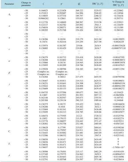
=Rs⋅2634.49.6. Sensitivity Analysis
We study the effects of changes in the parameters of the model such as A0, a, b, c, α , β, γ, Ch, Cp,
l
C , χv and δ on the optimal shortage point, the optimal length of the cycle, the optimal order quantity and
para-meters by −50%, −25%, +25% and +50% taking one parameter at a time while keeping others unchanged. The results are illustrated in Table 1 from Example-1.
Table 1. Sensitivity analysis.
Parameter Change in parameter
* 1
t *
T Q*0 ( )
* 1,
TRC t T % Change in *( ) 1,
TRC t T
0 A +50 +25 −25 −50 0.166023 0.151813 0.118055 0.0966262 0.221828 0.202687 0.157334 0.12863 268.222 244.906 189.797 155.015 3229.52 2946.85 2280.32 1860.71 +0.225862 +0.118566 −0.134436 −0.293711 a +50 +25 −25 −50 0.111726 0.122117 0.156034 0.188205 0.148849 0.162782 0.208371 0.251768 268.567 245.092 189.562 154.426 3219.38 2941.3 2287.82 1880.56 +0.222013 +0.116459 −0.131589 −0.286143 b +50 +25 −25 −50 0.136386 0.13674 0.18194 0.182416 219.179 219.259 2631.04 2627.58 −0.00130955 −0.0026229 c +50 +25 −25 −50 0.135974 0.136005 0.181387 0.181429 219.06 219.082 2634.9 2634.7 +0.000155628 +0.0000797118 α +50 +25 −25 −50 0.136379 0.136208 0.135866 0.135695 0.181733 0.181602 0.18134 0.181209 219.418 219.261 218.945 218.788 2630.08 2632.28 2636.69 2638.89 −0.00167395 −0.000838872 +0.000835076 +0.00167015 β +50 +25 −25 −50 0.135028 Complex no. Complex no. 0.134304 0.180706 Complex no. Complex no. 0.18012 218.183 217.475 2647.96 2655.55 +0.00511294 +0.00799396 γ +50 +25 −25 −50 0.136467 0.136251 0.135822 0.135609 0.181811 0.181641 0.181301 0.181133 219.513 219.308 218.898 218.695 2629.51 2632.0 2636.97 2639.45 −0.00189031 −0.000945154 +0.000941359 +0.00188272 h C +50 +25 −25 −50 0.104755 0.11807 0.162146 0.205308 0.157596 0.167553 0.202547 0.239134 189.677 201.953 245.073 290.215 3041.32 2857.33 2355.91 1989.44 +0.154425 +0.0845856 −0.105743 −0.244848 p C +50 +25 −25 −50 0.136375 0.136206 0.135868 0.135699 0.18173 0.1816 0.181341 0.181213 219.422 219.262 218.943 218.785 2630.1 2632.3 2636.68 2638.86 −0.00166636 −0.00083128 +0.00083128 +0.00165877 b C +50 +25 −25 −50 0.140474 0.13852 0.132776 0.128302 0.175595 0.178133 0.186057 0.192758 212.21 215.195 224.442 232.186 2720.32 2682.51 2571.47 2485.05 +0.0325794 +0.0182274 −0.0239211 −0.0567245 l C +50 +25 −25 −50 0.138628 0.137418 0.134443 0.132586 0.17799 0.179597 0.183682 0.186332 215.027 216.911 221.681 224.761 2684.61 2661.21 2603.69 2567.8 +0.0190246 +0.0101424 −0.0116911 −0.0253142 v χ +50 +25 −25 −50 0.136036 0.136036 0.136036 0.136037 0.18147 0.181471 0.181471 0.181471 219.102 219.103 219.103 219.103 2634.49 2634.49 2634.49 2634.48 0 0 0 6 3.7958 10−
− × δ +50 +25 −25 −50 0.138506 0.137349 0.134532 0.132791 0.178301 0.179775 0.183443 0.185768 215.117 216.963 221.612 224.597 2682.29 2659.9 2605.38 2571.68 +0.0181439 +0.00964513 −0.0110496 −0.0238414
1) t1*, *
T , Q0* &
(
)
*1,
TRC t T increase with increase in the value of the parameter A0. Here * 1 t , T*, *
0
Q & TRC t T*
(
1,)
are all highly sensitive to changes in A0. 2) t1* &*
T decrease while Q0* &
(
)
*1,
TRC t T increase with increase in the value of the parameter a. Here t1*,
*
T , Q0* &
(
)
*1,
TRC t T are all moderately sensitive to changes in a. 3) t1*,
*
T & Q0* decrease while
(
)
*1,
TRC t T increases with increase in the value of the parameter b for the first two values. Here t1*,
*
T , Q0* &
(
)
*1,
TRC t T are all lowly sensitive to changes in b. 4) t1*,
*
T & Q0* decrease while
(
)
*1,
TRC t T increases with increase in the value of the parameter c for the first two values. Here t1*,
*
T , Q0* &
(
)
*1,
TRC t T are all lowly sensitive to changes in b. 5) t1*,
*
T & Q0* increase while
(
)
*1,
TRC t T decreases with increase in the value of the parameter α for the last two values. Here t1*,
*
T , Q0* &
(
)
*1,
TRC t T are all lowly sensitive to changes in α . 6) t1*,
*
T & Q0* increase while
(
)
*1,
TRC t T decreases with increase in the value of the parameter β for the first and last values only. Here t1*,
*
T , Q0* &
(
)
*1,
TRC t T are all lowly sensitive to changes in β . 7) t1*,
*
T & Q0* increase while
(
)
*1,
TRC t T decreases with increase in the value of the parameter γ for the last two values. Here t1*,
*
T , Q0* &
(
)
*1,
TRC t T are all lowly sensitive to changes in γ . 8) t1*,
*
T & Q0* decrease while
(
)
*1,
TRC t T increases with increase in the value of the parameter Ch
for the last two values. Here t1*, *
T , Q0* &
(
)
*1,
TRC t T are all highly sensitive to changes in Ch.
9) t1*, *
T & Q0* increase while
(
)
*1,
TRC t T decreases with increase in the value of the parameter Cp for the last two values. Here t1*,
*
T , Q0* &
(
)
*1,
TRC t T are all lowly sensitive to changes in Cp. 10) t1* &
(
)
* 1,
TRC t T increase while T* & Q0* decrease with increase in the value of the parameter
b
C for the last two values. Here t1*, *
T , Q0* &
(
)
*1,
TRC t T are all moderately sensitive to changes in Cb.
11) t1* &
(
)
*1,
TRC t T increase while T* & Q0* decrease with increase in the value of the parameter Cl
for the last two values. Here t1*, *
T , Q0* &
(
)
*1,
TRC t T are all moderately sensitive to changes in Cl.
12) t1*, *
T & Q0* decrease while
(
)
*1,
TRC t T increases with increase in the value of the parameter χv
for the last two values. Here t1*, *
T , Q0* &
(
)
*1,
TRC t T are all lowly sensitive to changes in χv.
13) t1* &
(
)
*1,
TRC t T increase while T* & Q0* decrease with increase in the value of the parameter δ for the last two values. Here t1*,
*
T , Q0* &
(
)
*1,
TRC t T are all lowly sensitive to changes in δ.
7. Conclusions
In the present paper, an optimal policy for deteriorating items is derived considering quadratic demand rate, a three-parameter Weibull distribution deterioration rate and salvage value. Shortages are permitted and partially backlogged. The backlogging rate is dependent on the waiting time for the next replenishment. Quadratic de-mand is appropriate for the seasonal fashion items, cosmetic and high-tech products. As deterioration rate starts after some time when the items are stocked. Therefore, a three-parameter Weibull distribution deterioration rate is considered for developing the model. For selling the deteriorated units, salvage value is required for the termination of optimal total cost. Finally, optimal order quantity per cycle and optimal total relevant cost is de-rived. Shortages are not permitted and partially backlogged. As the rate of deterioration of most items increases with time or age, i.e., the longer the item remains unused, the higher would be its failure rate. Moreover, the lo-cation parameter illustrates the shelf-life of the item in the stock. Therefore, the three-parameter Weibull distri-bution deterioration is suitable for items with any initial value of the rate of deterioration and for items, which start deteriorating only after a certain period of time.
The proposed model can be extended in numerous ways. Firstly, we may extend demand rate to stock depen-dent demand rate. Secondly, it may be extended to stochastic demand pattern. Finally, we could also extend the model by incorporating quantity discounts, inflation, a finite rate of replenishment and permissible delay in payments etc.
References
[1] Harris, F.W. (1913) How Many Parts to Make at Once. Factory, the Magazine of Management, 10, 135-136. [2] Whitin, T.M. (1953) The Theory of Inventory Management. Princeton University Press, Princeton, 62-72.
[3] Ghare, P.N. and Schrader, G.F. (1963) A Model for Exponentially Decaying Inventories. The Journal of Industrial En-gineering, 15, 238-243.
[5] Aggarwal, S.P. (1987) A Note on an Order-Level Inventory Model for a System with Constant Rate of Deterioration,
Opsearch, 15, 184-187.
[6] Covert, R. and Philip, G.C. (1973) An EOQ Model for Items with Weibull Distribution. AIIE Transactions, 5, 323-326.
http://dx.doi.org/10.1080/05695557308974918
[7] Philip, G. C. (1974) A Generalized EOQ Model for Items with Weibull Distribution. AIIE Transactions, 6, 159-162.
http://dx.doi.org/10.1080/05695557408974948
[8] Misra, R.B. (1975) Optimum Production Lot-Size Model for a System with Deteriorating Inventory. International Journal of Production Research, 13, 495-505. http://dx.doi.org/10.1080/00207547508943019
[9] Raafat, F. (1991) Survey of Literature on Continuously Deteriorating Inventory Models. Journal of the Operational Research Society, 42, 27-37. http://dx.doi.org/10.1057/jors.1991.4
[10] Goyal, S.K. and Giri, B.C. (2001) Recent Trends in Modeling of Deteriorating Inventory. European Journal of Opera-tional Research, 134, 1-16. http://dx.doi.org/10.1016/S0377-2217(00)00248-4
[11] Li, R., Lan, H. and Mawhinney, J.R. (2010) A Review on Inventory Study. Journal of Service Science and Manage-ment, 3, 117-129. http://dx.doi.org/10.4236/jssm.2010.31015
[12] Bakker, M., Riezebos, J. and Teunter, R.H. (2012) Review of Inventory System with Deterioration since 2001. Euro-pean Journal of Operational Research, 221, 275-284. http://dx.doi.org/10.1016/j.ejor.2012.03.004
[13] Murdeshwar, T.M. (1988) Inventory Replenishment Policy for Linearly Increasing Demand Considering Shortages— An Optimal Solution. Journal of the Operational Research Society, 39, 687-692.
http://dx.doi.org/10.1057/jors.1988.116
[14] Goyal, S.K., Morrin, D. and Nebebe, P. (1992) The Finite Horizontal Trended Inventory Replenishment Problem with Shortages. Journal of the Operational Research Society, 43, 1173-1178. http://dx.doi.org/10.1057/jors.1992.183
[15] Chakrabarti, T. and Chaudhuri, K.S. (1997) An EOQ Model for Deteriorating Items with a Linear Trend in Demand and Shortages in All Cycles. International Journal of Production Economics, 49, 205-213.
http://dx.doi.org/10.1016/S0925-5273(96)00015-1
[16] Salameh, M.K., Fakhreddine, S.A. and Noueihed, N. (1999) Effect of Deteriorating Items on the Instantaneous Reple-nishment Model with Backlogging. Computers and Industrial Engineering, 37, 261-264.
http://dx.doi.org/10.1016/S0360-8352(99)00069-8
[17] Zhou, W.Y. and Lau, H.S. (2000) An Economic Lot-Size Model for Deteriorating Items with Lot-Size Dependent Replenishment Cost and Time-Varying Demand. Applied Mathematical Modelling, 24, 761-770.
http://dx.doi.org/10.1016/S0307-904X(00)00015-9
[18] Chang, H.J. and Dye, C.Y. (1999) An EOQ Model for Deteriorating Items with Time Varying Demand and Partial Backlogging. Journal of the Operational Research Society, 50, 1176-1182.
http://dx.doi.org/10.1057/palgrave.jors.2600801
[19] Papachristos, S. and Skouri, K. (2000) An Optimal Replenishment Policy for Deteriorating Items with Time-Varying Demand and Partial Exponential Type Backlogging. Operations Research Letters, 27, 175-184.
http://dx.doi.org/10.1016/S0167-6377(00)00044-4
[20] Abad, P.L. (2001) Optimal Price and Order Size for a Reseller under Partial Backordering. Computers and Operations Research, 28, 53-65. http://dx.doi.org/10.1016/S0305-0548(99)00086-6
[21] Teng, J.T., Yang, H.J. and Ouyang, L.Y. (2003) On an EOQ Model for Deteriorating Items with Time-Varying De-mand and Partial Backlogging. Journal of the Operational Research Society, 54, 432-436.
http://dx.doi.org/10.1057/palgrave.jors.2601490
[22] Sana, S. (2010) Optimal Selling Price and Lot-Size with Time Varying Deterioration and Partial Backlogging. Applied Mathematics and Computation, 217, 185-194. http://dx.doi.org/10.1016/j.amc.2010.05.040
[23] Roy, M., Sana, S. and Chaudhuri, K.S. (2011) An Economic Order Quantity Model of Imperfect Quality Items with Partial Backlogging. International Journal of Systems Science, 42, 1409-1419.
http://dx.doi.org/10.1080/00207720903576498
[24] Singh, T. and Pattnayak, H. (2013) An EOQ Model for Deteriorating Items with Linear Demand, Variable Deteriora-tion and Partial Backlogging. Journal of Service Science and Management, 6, 186-190.
http://dx.doi.org/10.4236/jssm.2013.62019
[25] Silver, E.A. and Meal, H.C. (1969) A Simple Modification of the EOQ for the Case of a Varying Demand Rate. Pro-duction and Inventory Management, 10, 52-65.
[26] Donaldson, W.A. (1977) Inventory Replenishment Policy for a Linear Trend in Demand—An Analytic Solution. Op-erational Research Quarterly, 28, 663-670. http://dx.doi.org/10.1057/jors.1977.142
[27] Dave, U. and Patel, L.K. (1981) (T, Si) Policy Inventory Model for Deteriorating Items with Time Proportional
[28] Giri, B.C., Goswami, A. and Chaudhuri, K.S. (1996) An EOQ Model for Deteriorating Items with Time Varying De-mand and Costs. Journal of Operational Research Society, 47, 1398-1405. http://dx.doi.org/10.1057/jors.1996.175
[29] Ghosh, S.K. and Chaudhuri, K.S. (2006) An EOQ Model with a Quadratic Demand, Time-Proportional Deterioration and Shortages in All Cycles. International Journal of Systems Sciences, 37, 663-672.
http://dx.doi.org/10.1080/00207720600568145
[30] Khanra, S., Ghosh, S.K. and Chaudhuri, K.S. (2011) An EOQ Model for a Deteriorating Item with Time Dependent Quadratic Demand under Permissible Delay in Payment. Applied Mathematics and Computation, 218, 1-9.
http://dx.doi.org/10.1016/j.amc.2011.04.062
[31] Singh, T. and Pattnayak, H. (2013) An EOQ Model for a Deteriorating Item with Time Dependent Quadratic Demand and Variable Deterioration under Permissible Delay in Payment. Applied Mathematical Sciences, 59, 2939-2951. [32] Singh, T., Pattanayak, H., Nayak, A.K. and Sethy, N.N. (2016) An EOQ Inventory Model with Stock Dependent
De-mand under Permissible Delay in Payment. International Journal of Logistics Systems and Management, Article in Press.
[33] Bhunia, A.K. and Maiti, M. (1999) An Inventory Model of Deteriorating Items with Lot-Size Dependent Replenish-ment Cost and a Linear Trend in Demand. Applied Mathematical Modelling, 23, 301-308.
http://dx.doi.org/10.1016/S0307-904X(98)10089-6
[34] Jalan, A., Giri, R. and Choudhury, K. (1996) EOQ Model for Items with Weibull Distribution Deterioration, Shortages and Trended Demand. International Journal of Systems Science, 27, 851-856.
http://dx.doi.org/10.1080/00207729608929285
[35] Ain, S. and Kumar, M. (2007) An EOQ Inventory Model of with Ramp Type Demand, Weibull Distribution Deteriora-tion and Starting with Shortage. Opsearch, 44, 243-260.
[36] Singh, T. and Pattnayak, H. (2013) An EOQ Inventory Model for Deteriorating Items with Varying Trapezoidal Type Demand Rate and Weibull Distribution Deterioration. Journal of Information and Optimization Sciences, 34, 341-360.
http://dx.doi.org/10.1080/02522667.2013.838445
[37] Chakrabarti, T., Giri, B.C. and Chaudhuri, K.S. (1998) An EOQ Model for Items with Weibull Distribution Deteriora-tion, Shortages and Trended Demand: An Extension of Philip’s Model. Computer and Operation Research, 25, 649- 657. http://dx.doi.org/10.1016/S0305-0548(97)00081-6
[38] Jain, S. and Kumar, M. (2010) An EOQ Inventory Model for Items with Ramp Type Demand, Three-Parameter Wei-bull Distribution Deterioration and Starting with Shortage. Yugoslav Journal of Operational Research, 20, 249-259.
http://dx.doi.org/10.2298/YJOR1002249J
[39] Jaggi, C.K. and Aggarwal, S.P. (1996) EOQ Model for Deteriorating Items with Salvage Values. Bulletin of Pure and Applied Science, 15, 67-71.
[40] Mishra, P. and Shah, N.H. (2008) Inventory Management of Time Dependent Deteriorating Items with Salvage Value.
Applied Mathematical Sciences, 16, 793-798.
[41] Annadurai, K. (2013) An Optimal Replenishment Policy for Decaying Items with Shortages and Salvage Value. Inter-national Journal of Management Science and Engineering Management, 8, 38-46.
Submit or recommend next manuscript to SCIRP and we will provide best service for you:
Accepting pre-submission inquiries through Email, Facebook, LinkedIn, Twitter, etc. A wide selection of journals (inclusive of 9 subjects, more than 200 journals) Providing 24-hour high-quality service
User-friendly online submission system Fair and swift peer-review system
Efficient typesetting and proofreading procedure
Display of the result of downloads and visits, as well as the number of cited articles Maximum dissemination of your research work