http://wrap.warwick.ac.uk/
Original citation:
Jhumka, Arshad, Bradbury, Matthew and Saginbekov, Sain. (2014) Efficient
fault-tolerant collision-free data aggregation scheduling for wireless sensor networks. Journal
of Parallel and Distributed Computing, Volume 74 (Number 1). pp. 1789-1801.
Permanent WRAP url:
http://wrap.warwick.ac.uk/64379
Copyright and reuse:
The Warwick Research Archive Portal (WRAP) makes this work of researchers of the
University of Warwick available open access under the following conditions. Copyright ©
and all moral rights to the version of the paper presented here belong to the individual
author(s) and/or other copyright owners. To the extent reasonable and practicable the
material made available in WRAP has been checked for eligibility before being made
available.
Copies of full items can be used for personal research or study, educational, or
not-for-profit purposes without prior permission or charge. Provided that the authors, title and
full bibliographic details are credited, a hyperlink and/or URL is given for the original
metadata page and the content is not changed in any way.
Publisher statement:
NOTICE: this is the author’s version of a work that was accepted for publication in
Journal of Parallel and Distributed Computing .Changes resulting from the publishing
process, such as peer review, editing, corrections, structural formatting, and other quality
control mechanisms may not be reflected in this document. Changes may have been
made to this work since it was submitted for publication. A definitive version was
subsequently published in
http://dx.doi.org/10.1016/j.jpdc.2013.09.011
A note on versions:
The version presented here may differ from the published version or, version of record, if
you wish to cite this item you are advised to consult the publisher’s version. Please see
the ‘permanent WRAP url’ above for details on accessing the published version and note
that access may require a subscription.
Efficient Fault-Tolerant Collision-Free Data Aggregation Scheduling for Wireless
Sensor Networks
I,IIArshad Jhumkaa,1,∗, Matthew Bradburya, Sain Saginbekova
aDepartment of Computer Science
University of Warwick Coventry CV4 7AL, UK
IThis work was supported by a grant from the University of Warwick.
IIThis is an extended version of a paper [18] that was published in the Proceedings of the Symposium on Reliable Distributed Systems (SRDS), 2010. ∗Corresponding author
Email addresses:[email protected](Arshad Jhumka),[email protected](Matthew Bradbury),
Abstract
This paper investigates the design of fault-tolerant TDMA-based data aggregation scheduling (DAS) protocols for wireless
sensor networks (WSNs). DAS is a fundamental pattern of communication in wireless sensor networks where sensor nodes
aggregate and relay data to a sink node. However, any such DAS protocol needs to be cognisant of the fact that crash failures
can occur. We make the following contributions: (i) we identify a necessary condition to solve the DAS problem, (ii) we
introduce a strong and weak version of the DAS problem, (iii) we show several impossibility results due to the crash failures
(iv) we develop a modular local algorithm that solvesstabilising weak DASand (v) we show, through simulations and an actual
deployment on a small testbed, how specific instantiations of parameters can lead to the algorithm achieving very efficient
stabilization.
1. Introduction
Data gathering is a basic capability expected of any wireless sensor network (WSN). The usual way of performing data
gathering is to have nodes send their measurements (possibly over multiple hops) to a particular node called asink. This type
of communication, calledconvergecast, is fundamental to WSNs. Convergecast generally works by constructing a logical tree
(called a convergecast tree) on top of the physical topology, with the sink located at the root, and data is then routed to the sink
along the tree. However, to save energy, the data is typically aggregated along the route at specific nodes. This means that
an aggregator node needs to have all the values from its children before aggregating the data. However, due to the broadcast
nature of the communication medium, data transmissions need to be mediated among the children (and possibly other nodes)
to avoid message collisions and interference, events that typically lead to energy exhaustion and which could also bias the
aggregation.
Mediating these transmissions can be achieved through the use of an appropriate media access control (MAC) protocol.
For WSN applications that need fast response times (e.g., disaster recovery), timeliness is of utmost importance. To this end,
we investigateTime Division Multiple Access (TDMA)-based MAC protocols for data aggregation scheduling, in which each
node is allocated a specific time slot in which it can transmit its data. Another advantage of a TDMA schedule for WSNs is
that the transceivers can be turned on only when needed, thus saving energy. There exist several algorithms for convergecast
in multi-hop radio networks, e.g., [19, 15, 23] that can be used for WSNs. A common pattern in TDMA-based convergecast
algorithms is the decomposition of the problem into two independent subproblems: (i) a logical tree construction, and (ii)
time slot allocation along the constructed tree. For example, the tree in [19] is constructed based on the positions of the
nodes in a 2-D plane. Various objectives of convergecast scheduling algorithms exist, e.g., minimizing time for completing a
convergecast [15], maximizing throughput [23], which determine the slot assignment (i.e., the schedule) along the tree.
When slots are assigned to nodes for data aggregation, in what we term asdata aggregation scheduling(DAS), a node will
first aggregate the data obtained from its children before relaying it to its parent. The objective, in this case, is that a node can
only transmit a messageaftercollecting data fromallof its children. However, whenever a node crashes in a WSN (e.g., due
to energy depletion), the values from a whole subtree disappears. Thus, it is important for a DAS algorithm to be fault-tolerant
to ensure that correct nodes have a proper path to the sink, in the sense that their parent transmits the aggregated data after
their own transmission.
1.1. Contributions
Several work has addressed the problem of convergecast, with a subset of these addressing the problem of data aggregation
scheduling. However, to the best of our knowledge, no work has investigated the problem ofDAS in presence of crash
failures, on which we focus in this paper. Crash failures in WSNs can be brought about by, for example, defective hardware
or battery exhaustion. In this context, we make an in-depth study of DAS in presence of crash failures. We make a number of
contributions in three categories:
• Theory
1. We identify a necessary condition for solving the data aggregation scheduling problem. This condition provides
the theoretical basis that explain the structure of several data aggregation scheduling.
3. We show that it is impossible to solve the strong data aggregation scheduling problem.
4. We show that it is impossible to solve the weak data aggregation scheduling problem in presence of crash failures.
5. We introduce the problem of stabilising weak data aggregation scheduling and show that, in general, there is no
2-local algorithm that solves the problem.
• Algorithm
1. We develop a modulard-local algorithm that solves weak DAS and achieves efficient stabilization, wheredis the
diameter of the affected area.
• Results and Validation
1. Using both simulation and an actual deployment on a small testbed, we show that, under appropriate
parameteri-zation, thed-local algorithm can achieve2-local stabilization.
Our paper is structured as follows: We present our system and fault models in Section 2. We formalize the problems of
strong and weak data aggregation scheduling in Section 3. In Section 4, we focus on variants of the weak data aggregation
convergecast. In Section 5, we present and prove the various impossibility results. In Section 6, we provide ad-local algorithm
that achieves efficient stabilization. We present the performance of our algorithm in Section 7. In Section 8, we survey related
work in the area, and put our work in the proper context. We discuss the impact of the results in Section 9. We finally
summarise the paper in Section 10.
2. Models: System and Faults
2.1. Graphs and networks:
A wireless sensor node is a computing device that is equipped with a wireless interface and is associated with a unique
identifier. A wireless sensor network (WSN) consists of a set of wireless sensor nodes that communicate among themselves
via their wireless interface. Communication in wireless networks is typically modelled with a circular communication range
centered on a node. With this model, a node is thought as able to exchange data with all devices within its communication
range.
A wireless sensor network is then typically modelled as an undirected graphG= (V, E)whereV is a set ofΓwireless
sensor nodes andE is a set of edges or links, each link being a pair of distinct nodes. Two nodesm, n∈ V are said to be
1-hop neighbours (or neighbours) iff(m, n)∈E, i.e.,mandnare in each other’s communication range. We denote byM
the set ofm’s neighbours, and we denote byMd, thed-hop neighbourhood ofm. We say that two nodesmandncan collide
at nodepif(p∈M)∧(p∈N)2. In general, two nodesmandncan collide if they are in the 2-hop neighbourhood of each
other. We then define the collision group of a nodenas follows:
CG(n) ={m∈V|((n, m)∈E)∨(2hopN(m, n))},
where2hopN(m, n)is a predicate that returns true ifm, nare in each other’s 2-hop neighbourhood.
We denote by ∆m the degree of node m, i.e., the size ofM. We also denote by∆G, the degree of G, i.e., ∆G =
max({∆m, m∈V}). We also denote byηG, the maximum of nodes at any hop distance inG. We assume a distinguish node
S∈V, called asink. A path of lengthkis a sequence of nodesnk. . . n0such that∀j,0< j≤k,njandnj−1are neighbours.
We say a pathnk. . . n0is anS-path ifn0=S. The pathnk. . . n0is said to beforwardif∀i, j,0< i≤j ≤k, ni 6=nj. A
pathnk. . . n0is called acycleif the path is forward andn0 =nk. In this paper, we focus on forwardS-paths (henceforth,
paths). Specifically, we are only interested in paths from a node to the sink, hence forwardS-paths. For anS-pathnk. . . S,
we say thatnkhas anS-path.
Given an undirected graphG= (V, E): Gis connected iff there exists a path inGbetween each pair of distinct nodes.
In general, we are only interested in paths that end with the sink. We say thatGis S-connected iff every node inGhas
anS-path, and we say thatGisSk-connected iffGisS-connected, and all nodes haveknode-disjointS-paths. Two paths
are node-disjoint only if the end nodes of the two paths are the same while all other nodes differ. In this paper, when we
mention disjoint paths, we mean node-disjoint paths. The distance between two nodesmandninGis the length of the
smallest path betweenmandninG. We denote the distance betweenmandnbyd(m, n). The diameterDGofGis equal
to max({d(m, n), m∈V ∧n∈V}).
2.2. Distributed programs
2.2.1. Syntax
We model the processing on a WSN node as a process containing non-empty sets of variables and actions. A distributed
program is thus a finite set ofNcommunicating processes. We represent the communication network topology of a distributed
program by an undirected connected graphG= (V, E), whereV is the set ofN processes andEis a set of edges such that
∀m, n∈V,(m, n)∈Eiffmandncan directly communicate together, i.e., nodesmandnare neighbours.
Variables take values from a fixed domain. We denote a variablev of processnbyn.v. Each processnhas a special
channel variablech, denoted byn.ch, modelling a FIFO queue of incoming data sent by other nodes. This variable is defined
over the set of (possibly infinite) message sequences. Every variable of every process, including the channel variable, has a
set of initial values. Thestateof a program is an assignment of values to variables from their respective domains. The set of
initial states is the set of all possible assignments of initial values to variables of the program. A state is called initial if it is in
the set of initial states. The state space of the program is the set of all possible value assignments to variables.
An action at a processphas the formhnamei::hguardi → hcommandi. In general, a guard is a state predicate defined
over the set of variables ofpand possibly ofp’s neighbours. When the guard of an action evaluates totruein a states, we say
the action is enabled ins3, and the correspondingcommandcan be executed, which takes the program from statesto another
states0, by updating variables of processp. We assume that the execution of any action is atomic. Acommandis a sequence
of assignment and branching statements. Also, aguardorcommandcan contain universal or existential quantifiers of the
form: (hquantif ierihbound variablesi : hrangei : htermi), whererangeandtermare boolean constructs. A special
timeout(timer) guard evaluates to true when a timer variable reaches zero, i.e., the timer expires. Aset(timer, value)
command can be used to initialise the timer variable to a specified value.
2.2.2. Semantics
We model a distributed programφas a transition systemφ= (Σ, I, τ), whereΣis the state space,I⊆Σthe set of initial
states, andτ⊆Σ×Σthe set of transitions (or steps). A computation ofφis a maximal sequence of statess0·s1. . .such that
s0∈I, and∀i >0,(si−1, si)∈τ. A statesis terminal if there is no states0such that(s, s0)∈τ. We denote reachability of
states0fromsass→∗s0, i.e., there exists a computation that starts fromsand containss0.
In a given states, several processes may be enabled, and a decision is needed to decide which one(s) execute. Ascheduler
is a predicate over the computations. In any computation, each step(s, s0)is obtained by the fact that a non-empty subset
of enabled processes insatomically execute an action. This subset is chosen according to the scheduler. A scheduler is
saidcentral[9] if it choosesonly oneenabled process to execute an action in any execution step. A scheduler is said to be
distributed [5] if it choosesat least oneenabled process to execute an action in any execution step. Oan the other hand, a
synchronous scheduler is a distributed scheduler whereallenabled processes are chosen to execute an action in a step.
A scheduler may also have some fairness properties [10]. A scheduler is strongly fairif every process that is enabled
infinitely often is chosen infinitely often to execute an action in a step. A scheduler is weakly fairif every continuously
enabled process is eventually chosen to execute an action in a step. In this paper, we assume a synchronous scheduler,
capturing a synchronous system where an upper bound exists on the time for a process to execute an action [21]. In other
words, it can capture systems where processes execute in a kind of lock-step fashion. This assumption is not unreasonable as
WSNs are often time-synchronized [25] to either correlate sensor readings from different devices or for time-based protocols
such as TDMA [16].
2.2.3. Specification
A specification is a set of computations. Programφsatisfiesspecification¶if every computation ofφis in¶. Alpern and
Schneider [1] stated that every computation-based specification can be described as the conjunction of a safety and liveness
property. Intuitively, a safety specification states that something bad should not happen, whereas a liveness specification states
that something good will eventually happen. Formally, the safety specification identifies a set of finite computation prefixes
that should not appear in any computation. A liveness specification identifies a set of computation suffixes such that every
computation has a suffix in this set.
2.2.4. Communication
An action with a rcv(msg, sender)guard is enabled at processpwhen there is a message at the head of the channel
p.ch, i.e.,p.ch6=hi. Executing the corresponding command causes the message to be dequeued from thep.ch, whilemsg
andsenderare bound to the content of the message and the identifier of the sender node. With a weak or strong fairness
assumption, a stand alonercv(msg, sender)guard implies that the messagemsgwill eventually be delivered. Differently,
theBCAST(msg)(orsend(msg)) command causes messagemsgto be enqueued to the channelq.chof all processesqthat
are neighbours ofp. We model synchronous communication as follows: after a processmsends a message to another process
nin statesi, the message is inn.chin statesi+1. Overall, in this paper, we assume a synchronous system model.
2.3. Faults
A fault model stipulates the way programs may fail. We considercrashfailures that causes a program to stop executing
instructions. Formally, a crash failure can be modeled through the use of auxiliary variables, and appropriate fault (crash)
wherep.up = 0means processphas crashed, andp.up = 1otherwise. A crash action changes the value of the auxiliary
variable. From the example, the crash action will change variableupfrom 1 to 0. A crash occurs if a crash action is executed.
Crash actions can interleave program actions and they might or might not be executed when enabled. We say a computation
is crash-affected if the computation contains program and crash transitions. In this paper, we assume that the sink node does
not crash. We also assume that any crash does not partition the network. A program isself-stabilizingiff, after faults have
stopped occurring, the program eventually reaches a state from where its specification is satisfied.
2.4. Time Division Multiple Access
TDMA is a technique whereby the timeline is split into a series of time periods (or periods), and each period is divided
into a series of time slots. In each period, every node is assigned a slot in which the node transmits its message. Slots have to
be assigned carefully to avoid message collisions. Specifically, nodes that are in each others’ collision groups cannot transmit
in the same slot.
Definition 1 (Non-colliding slot). Given a networkG, a noden ∈G, and a slotiin whichncan transmit its payload, we say thatiisnon-colliding forniff∀m∈CG(n)·m.slot6=i.
Definition 2 (F-affected node andF-affected area). Given a networkG= (V, E)and a faultFthat causes up tof crashes inG, a node is said to beF-affected(or affected) in a program state if the node will need to change its state to make the
program state consistent. AnF-affected area(or affected area) of a program state is a maximal set of connectedF-affected
nodes in that state.
Definition 3 (d-local self-stabilizing algorithm). Given a networkG= (V, E), a problem specification¶forG, and a self-stabilizing algorithmAthat solves¶. AlgorithmAis said to bed-local self-stabilizingfor¶iff, for every affected noden,
messages that correct the state of the affected node originate from itsNdneighbourhood.
3. Data Aggregation Scheduling Definitions
In this section, we present two variants of the data aggregation scheduling, namely (i) the strong data aggregation
schedul-ing, and (ii) the weak data aggregation scheduling. Recall that we are focusing on forwardS-paths, i.e., paths that end with a
sink. For data aggregation scheduling, as argued before, nodes closer to the sink should transmit later than nodes further away
from a sink (in what we call as proper slot assignment).
We first provide two definitions.
Definition 4 (Strongly and Weakly Proper Slot). Given a graphG= (V, E), a slotiallocated to a noden, i.e.,n∈ρi, is
said to bestrongly proper forninGif and only if∀m∈N, n·m . . . Sis a path:∃j > i:m∈ρj. Also, a slotiallocated to
a noden, i.e.,n∈ρi, is said to beweakly proper forninGif and only if∃m∈N, n·m . . . Sis a path:∃j > i:m∈ρj.
3.1. Strong Data Aggregation Scheduling
We define the problem of strong data aggregation scheduling problem. The intuition here is, in a network where up
to f crash failures can occur, there should be at least (f + 1) disjoint paths from any node to the sink for the network
to remain connected. Then, for strong DAS, we require that every path has a proper slot assignment, i.e., for every path
n . . . ni ·ni+1. . . S from a noden to sinkS, the slot for ni+1 is greater than the slot forni. Formally, the strong data
aggregation scheduling is defined as follows:
Definition 5 (Strong data aggregation scheduling). Given a networkG= (V, E), a strong TDMA-based collision-free data aggregation schedule is a sequence of sets of sendershρ1, ρ2, . . . , ρlisatisfying the following constraints:
1. ρi∩ρj =∅,∀i6=j,
2. Sli=1ρi=V \ {S},
3. ∀n∈ρ1≤i≤l−1:∀m∈N, n·m . . . Sis a path:(m∈ρj>i)∨(m=S),
4. ∀ρ1≤j≤l−1:∀m, n∈ρj:m6=n⇒n6∈CG(m)∧m6∈CG(n).
There are four conditions that capture the strong data aggregation scheduling problem. These conditions are explained
here:
1. The first condition stipulates that nodes are allocated at most one time slot in the schedule.
2. The second condition implies that all nodes (apart from the sink) will get at least one transmission slot. Taken together,
conditions 1 and 2 state that every node (except the sink) will transmit in exactly one slot in the schedule.
3. The third condition captures the fact that whenever a node transmits a message,allof its neighbours that are closer to
the sink will transmit in a later slot, and the condition captures the notion ofstrongly proper slots.
4. The last condition captures the condition for collision freedom, i.e., two nodes can transmit in the same slot only if they
are not in each other’s collision group.
Overall, nodes inρ1transmit first, followed by those inρ2, and so on, until those inρl. The parameterlis called the data
aggregationlatency. Observe that|ρl|= 1, since if|Pl| ≥1, there will be a message collision atS.
Given a networkG= (V, E), an algorithm that produces a slot assignment that satisfies the above requirements forGis
said to solve thecollision-free strong data aggregation scheduling(or simply the strong data aggregation scheduling) problem
forG, and the schedule is termed astrong proper schedule forG.
3.2. Weak Data Aggregation Scheduling
In this section, we formally define the problem of weak data aggregation scheduling.
Definition 6 (Weak data aggregation scheduling). Given a networkG= (V, E), a weak TDMA-based collision-free data
aggregation schedule is a sequence of sets of sendershρ1, ρ2, . . . , ρlisatisfying the following constraints:
1. ρi∩ρj =∅,∀i6=j,
2. Sli=1ρi=V \ {S},
3. ∀n∈ρ1≤i≤l−1:∃m∈N, n·m . . . Sis a path:(m∈ρj>i)∨(m=S),
As for the case of strong data aggregation scheduling, conditions 1 and 2, taken together, state that every node (except the
sink) will transmit in exactly one slot in the schedule. The third condition captures the fact that whenever a node transmits a
message,at least oneof its neighbours closer to the sink will transmit in a later slot, and the condition captures the notion of
weakly proper slots. The last condition captures the condition for collision freedom, as in the case of strong data aggregation
scheduling.
Given a networkG= (V, E), an algorithm that produces a schedule that satisfies the above requirements forGis said to
solve thecollision-free weak data aggregation schedulingproblem forG, and the schedule is termed aweak proper schedule
forG. Similarly, the parameterlis the latency of the data aggregation scheduling.
4. Data Aggregation Scheduling Specifications
Given the definition for weak data aggregation scheduling (Definition 6), there are possibly different ways of producing
a weakly proper schedule. In this paper, we focus on two specific ways, namely (i) a deterministic way, and (ii) a stabilising
way. These two possibilities capture two possible behaviours of algorithms that can generate a weakly proper data aggregation
schedule. The specifications are described following the notion that a trace-based specification is the intersection of a safety
specification and a liveness specification [1].
The two specifications we provide are similar in ideas to the notions of perfect failure detectors and eventually perfect
failure detectors, a la Chandra and Toueg [6], although in a very different context. Specifically, the deterministic specification
captures the fact that a node is only assigned a slot that is weakly proper and non-colliding, and that the slot is permanent, i.e.,
never changed. On the other hand, in the stabilising specification, we permit a node to change slots, with the exception that
eventually a weakly proper and non-colliding slot will be permanently assigned.
4.1. Deterministic Weak Data Aggregation Scheduling
In this section, we provide the specification fordeterministic weak data aggregation scheduling(Definition 7).
Definition 7 (Deterministic Weak DAS). Given a networkG = (V, E), a programA solves thedeterministic weak data aggregation schedulingproblem (Definition 6) forGif every computation ofAsatisfies the following:
1. Safety: A nodeninGis allocated a permanent slot only if the slot is weakly proper and non-colliding forninG.
2. Liveness: Eventually, every nodeninGis allocated a slot.
WheneverGis obvious from the context, we will omit its use. Safety prevents a node from being assigned any arbitrary
slot, while liveness requires every node to be eventually allocated a slot. Taken together, it captures the notion that all nodes
will eventually be permanently allocated non-colliding weakly proper slots, which then generate the weak data aggregation
schedule forG.
4.2. Stabilising Weak Data Aggregation Scheduling
We now define a weaker version of the deterministic specification, namely the stabilising version (Definition 8).
1. Safety: Eventually, a nodeninGis permanently allocated a slot only if the slot is weakly proper and non-colliding for
ninG.
2. Liveness: Eventually, every nodeninGis allocated a slot.
The stabilising version of the data aggregation scheduling problem allows an algorithm Ato make a finite number of
mistakes during slot allocation (in contrast, no mistakes are allowed in the deterministic version). The mistakes may be due
to the fact that the slots allocated are not weakly proper, which could be due to topology changes, incomplete information
etc. Eventually, the mistakes will stop, for example when faults stop, and a weak data aggregation schedule will be eventually
obtained.
In the next section, we investigate the possibilities and impossibilities of achieving strong and weak data aggregation
convergecast schedules.
5. Research Contributions
In this section, we present some of the important research contributions we make in this paper. These are:
1. Our first contribution (Section 5.1) is the identification of a necessary condition that helps solve the strong or weak DAS
problem.
2. We then show, in Section 5.2, that it is impossible to solve the strong data aggregation scheduling problem.
3. In Section 5.3, we show that it is impossible to solve the deterministic weak data aggregation scheduling problem in
presence of crash failures.
4. We then show, in Section 5.4, that there exists no2-local algorithm that solves the stabilising proper DAS problem.
5.1. Necessary Condition to Solve Strong and Weak Data Aggregation Scheduling
Before attempting to solve the data aggregation scheduling problem, we wish to determine the type of information required.
In this context, our first main contribution is a necessary condition to solve the strong or weak DAS, as captured by Theorem 1.
IntuitionWhen a nodenhas to decide on a slot, it needs to determine which of its neighbours are on a path to the sink. If
a node cannot determine this, i.e., it cannot discriminate among its neighbours, then it is difficult fornto decide on a strongly
or weakly proper slot, thus the data aggregation scheduling problem becomes difficult to solve.
Theorem 1 (Necessary condition). Given a networkG= (V, E), there exists no deterministic algorithmAthat solves the strong/weak DAS problem if∃n∈(V \ {S}),ncannot choose a nodem∈Nsuch thatn·m . . . Sis a path.
Proof
We assume the existence of the algorithmAthat solves the strong/weak DAS problem when a nodencannot choose a
nodem∈N such thatn·m . . . Sis a path, and show a contradiction.
Given a graph G = (V, E). Assume a noden ∈ V \ {S} with neighbourhoodN, and a unique nodem ∈ N with
n·m . . . Sa path inG. SinceAsolves the weak/strong DAS problem,Aidentifiesm∈N as the neighbour on the path from
ntoS, withm.slot > n.slot.
Now, given another graphG0 = (V, E0), whereG0 differs fromGas follows: the nodes are labelled such thatNinG0is
deterministic,Awill again choosemas being on the path fromntoS(since nodes cannot determine which of its neighbour
is on the path toS). However, asm.slot > n.slot, then this violates the strong/weak DAS requirement. Hence,Acannot
exist.
Theorem 1 states that nodes need to be able to determine which node, among their neighbours, is on the path to the sink.
This is only an abstract requirement, and there can be various possible implementations for this. In fact, Theorem 1 provides
an insight into the design of existing convergecast and data aggregation scheduling algorithms [19, 15]. These algorithms
in [19, 15] indeed provided different possible implementations of the abstract requirement identified in Theorem 1. In [19],
the authors used classes of graphs (such as grids) and node locations to infer the direction of the sink and, hence, their
neighbours on anS-path. In [15], the authors used hop distance to allow a node to determine which of its neighbours is on the
path to the sink.
5.2. Strong Data Aggregation Scheduling
The scale and nature of wireless sensor networks often mean that failures of sensor nodes will not be rare events. Thus,
it is important for data aggregation and message relay to proceed in spite of these failures. Therefore, solving the strong data
aggregation scheduling problem is important as it enables any node to forward its aggregated data, in spite of various node
(hence path) failures. Our second major contribution is to determine the feasibility of obtaining a strong data aggregation
schedule, as captured by Theorem 2. The main implication of a strong data aggregation schedule is that, if a node has a
strongly proper slot, then the schedule is inherently resilient to a certain number of crash failures.
Intuition Given a networkG = (V, E)in which every node has at least two disjoint paths to the sink. Consider three nodesm, n, p∈V. Now, assume a pathr1forpisp·n·m . . . S, while a pathr2formism·n·p . . . S. From the definition of
strong data aggregation scheduling (Definition 5), if nodephas a strongly proper slot, then inr1, the slot ofnis greater than
that ofp. However, inr2, the slot ofnis smaller than that ofp, violating the strong data aggregation scheduling specification.
Theorem 2 (Impossibility - Strong DAS). Given a networkG= (V, E)in which every noden∈V has at least two disjoint paths to the sink. Then, there exists no deterministic algorithm that can generate a strong data aggregation schedule.
Proof
We assume the existence of the algorithm A that can generate a strong data aggregation schedule, and then show a
contradiction.
Consider three nodesm, n, p∈V, and they haverm, rn, rp≥2disjointS-paths respectively. Assume thatm·n·p . . . S
is a path inG. SinceAgenerates a strong data aggregation schedule, then the slot fornis greater than the slot for nodem.
Now, sincerm≥2and one path formism·n·p . . . S, then there exists a path forpinGsuch thatp·n·m . . . S. On
this path, sinceAgenerates a strong data aggregation schedule, then the slot assigned tonis less than that assigned to node
m. This is a contradiction from the previous observation. Hence,Acannot exist.
The implication of Theorem 2 is that it is impossible, in general, to generate a strong data aggregation schedule. On the
other hand, it can be observed that a weak data aggregation schedule can be generated. However, understanding the generation
of weak data aggregation schedules in presence of crash failures is important, so as to capture the resilience of such schedules,
5.3. Deterministic Weak Data Aggregation Scheduling in presence of Crash
In this section, we investigate the possibility of solving the deterministic weak data aggregation scheduling problem in
presence of crash failures, where nodes stop executing program instructions. To the best of our knowledge, no work has
addressed the problem of weak data aggregation scheduling problems in the presence of crash failures. We show that it is
impossible to solve the deterministic weak data aggregation scheduling problem in presence of crash failures.
IntuitionFrom the specification of deterministic weak DAS, it is stated that nodes are only ever assigned weakly proper slots. However, when a node is being assigned a weakly proper slot and a crash failure occurs along the relevant pathr(which
makes the slot weakly proper), then the slot is no longer weakly proper asrno longer exists.
Thus, the third main contribution of the paper is captured by Theorem 3, which states that it is impossible to solve
deterministic weak data aggregation scheduling in presence of crash failures. From Theorem 1, we assume that nodes can
determine which of their neighbours are on the path to the sink.
Theorem 3 (Impossibility - Deterministic Weak DAS). Given a networkG = (V, E)in which every noden ∈ V has at
least (f+ 1) disjoint paths to the sink, a fault modelFwhere up tof crash failures can occur. Then, there exists no algorithm
that can solve the deterministic weak data aggregation scheduling problem forGin the presence ofF.
Proof
Assume an algorithmAthat solves the deterministic weak data aggregation scheduling problem forG, and show a
con-tradiction.
Consider three nodes m, n, p ∈ V, and they have rm, rn, rp ≥ f + 1S-paths respectively. Assume that (m·n1 ·
p1. . . S). . .(m·nrm ·prm. . . S)are thermpaths forminG. Consider a statesin a computationσofA, where nodemis
assigned a weakly proper slot (for all the paths(m·n2·p2. . . S). . .(m·nf+1·pf+1. . . S)), i.e., nodemhas a slot which is
less than those of nodesn2. . . nf+1, resulting in states0.
Now, consider a faulty computationσ0ofAwhich is identical toσup to states. In states, nodesp2. . . pf+1crash. Since
σ0 is identical toσup tosandAis deterministic, then nodemchooses a slot which is less than that of nodesn2. . . nf+1,
resulting is states0. However, because of nodesp2. . . pf+1crashing, the paths(m·n2·p2. . . S). . .(m·nf+1·pf+1. . . S)
no longer exist. Hence, the slot for nodenis no longer weakly proper forG0, which is identical toGexcept without nodes
p2. . . pf+1. Hence,Adoes not assign a weakly proper slot tominσ0, which is a contradiction. Hence, no suchAexists.
Theorem 3 states that, in presence of crash failures, it is impossible to solve the deterministic weak data aggregation
scheduling problem. Specifically, this happens due to the fact that nodes can mistakenly be assigned slots that are not weakly
proper, due to the crash failures, as the nodes are unaware of the failures when they are choosing slots. Thus, to allow for
these possible mistakes to be corrected, we weaken the specification, and consider the stabilising version of the problem, viz.
stabilising weak data aggregation scheduling problem. The area of self-stabilisation is quite mature [10]. A self-stabilising
algorithm is one that eventually satisfies its specification, in the sense that the safety property is eventually satisfied. In the next
section (Section 5.4), we investigate on the possibility of achieving stabilising weak data aggregation scheduling in presence
of crash failures.
5.4. Stabilising Weak Data Aggregation Scheduling in presence of Node Crashes
Because mistakes can be made during slot assignment due to node crashes, the specification for stabilising weak data
slots, allowing a finite number of mistakes to be made. From Theorem 1, we know that nodes only need to know at least
one of their neighbours on a path to the sink. Thus, we investigate the problem of whether a2-local algorithm can solve the
stabilising weak data aggregation scheduling, i.e., achieving stabilising weak data aggregation scheduling using information
about the2-hop neighbourhood only.1-local algorithms cannot be used as collision-free TDMA scheduling needs distance-2
colouring type algorithms. 2-local algorithms are important as they make use of local interactions only [17], thus helping
reduce energy consumption, thereby prolonging network lifetime.
IntuitionIn the specification for stabilising weak data aggregation scheduling, nodes are allowed to make a finite number of mistakes when deciding on proper slots. However, since a crash can happen beyond the2-hop neighbourhood of a node,
then the information held by a node needs to be beyond its 2-hop neighbourhood. Hence, solving stabilising weak data
aggregation scheduling by2-local algorithms is impossible. Specifically, a node needs to have a network wide information
about crashes to determine which of its neighbouring nodes has a path to the sink. This is captured by Theorem 4.
Theorem 4 (Impossibility). Given a networkG= (V, E)in which every noden∈V has at least (f + 1) disjoint paths to the sink, a fault modelF where up tof crash failures can occur. Then, there exists no2-local algorithm that can solve the
stabilising weak DAS problem in the presence ofF.
Proof:
We assume an algorithmAthat solves the stabilizing weak data aggregation scheduling problem and that is2-local, and
show a contradiction.
Consider a nodem∈V, and it hasrm≥f+ 1S-paths respectively. Assume that(m·n1·p1·c1. . . S). . .(m·nrm·prm·
crm. . . S)are thermdisjoint paths forminG. Consider a statesin a computationσofA, where the following happens:
(i) nodemis assigned a weakly proper slot for the pathm·n1·p1·c1. . . S only, i.e., nodemhas a slot which is less than
that of node n1 and (ii) node c1 crashes, resulting in state s0. Now, nodem does not have a weakly proper slot, as path
m·n1·p1·c1. . . Sdoes not exist anymore.
SinceAsolves the stabilizing weak data aggregation scheduling problem, then there exists a states00> s0 where nodem
will have a weakly proper slot forG0 (similar toGwithout the crashed nodec1) again. To recompute a weakly proper slot,
nodemhas learnt about the crash of nodec1. However,c1was 3 hops away fromm, meaningAis a3-hop algorithm. This is
a contradiction. Hence, no suchAexists.
Since there is no2-local algorithm that can solve the stabilising weak data aggregation scheduling, it is obvious that a
d-local algorithm exists, wheredis the diameter of the affected region, since every node needs to know about node failures as
far away as where failures have occurred, i.e., up todhops away.
6. A Crash-Tolerant Collision-Free Data Aggregation Scheduling Algorithm
In this section, we present a modulard-local algorithm that solves for stabilizing weak data aggregation scheduling. We
will also show that, under specific parameterization, the algorithm can achieve2-local stabilisation.
6.1. An Efficientd-local Algorithm for Solving Stabilising Weak DAS
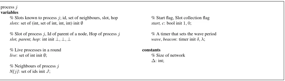
processj
variables
% Slots known to processj; id, set of neighbours, slot, hop slots: set of (int, set of int, int, int) init∅
% Slot of processj, Id of parent of a node, Hop of processj slot, parent, hop: int init⊥,⊥,⊥
% Live processes in a round live: set of int init∅;
% Neighbours of processj N[j]: set of ids initJ;
% Start flag, Slot collection flag start, c: bool init1,0;
% A timer that sets the wave period wave,beacon: timer initδ, λ;
constants
% Size of network
[image:15.612.59.557.109.252.2]∆: int;
Figure 1: Variables ofd-local algorithm that solves stabilising Weak DAS for a general network.
actions
%Diffusing slot information
dissem::timeout(wave)→ slots:=∅;
if(sink(j)∧(start= 1))then
BCASThj, N[j],Γ,0i;
start:= 0;
elseif(¬sink(j)∧(slot6=⊥))then
BCASThj, N[j]\ {parent},slot,hopi;
fi;
set(wave,δ);
%Sending neighbourhood info.
neighbourS::timeout(beacon)→
BCASThji;
set(beacon,λ);
%Collecting neighbourhood through beacon messages.
neighbourC::rcvhni → live:=live∪{n};
%Receiving information from neighbour nodes.
receive::rcvhn, N, s, hi →
c, live, slots:= 1,live∪{n},slots∪{(n, N, s, h)};
%Resolving slot conflicts.
resolve::rcvhcoll, Si →
if(j∈S∧slot6=⊥)then
slot:=slot−rank(j, S) + 1;
fi;
%All slots msgs processed.
check::rcvhi →
if(c6= 1∧parent6=⊥ ∧parent6∈live)then
slot, parent, hop:=⊥,⊥,⊥;
BCASThcrash, ji;
N[j]:= live;
fi;
if(c= 1)then
if(slot6=⊥)then
slots:=slots∪(j,N[j],slot,hop);
fi;
if(∃s· |{n|(n, N, s, h)}| ≥2)then
∀s· |{n|(n, N, s, h)}| ≥2 :
BCASThcoll,{n|(n, N, s, h)∈slots}i;
elseif(¬sink(j)∧(slot=⊥ ∨parent=⊥ ∨hop=⊥))then
hop:=min{h|(n, N, s, h)∈slots} + 1;
slot:=min{s|(n, N, s,hop−1)∈slots} −rank(j, N); parent:=choose{n|(n, N,slot+rank(j, N),hop−1)∈slots};
fi;
c:= 0;
fi;
live:=∅;
%Receiving crash information
reset::rcvhcrash, ii →
if(parent=i)then
slot, parent, hop:=⊥,⊥,⊥;
BCASThcrash, ji;
fi;
[image:15.612.58.560.310.665.2]VariablesEach processjruns a copy of the program, and the program has two timers: (i) awavetimer set toδ, and (ii) abeacontimer set toλ, and bothδandλare parameters of the program. Each process will keep track of itsparent, hop, slot
values, while the variableslotsstores information about the neighbours of processj. Variablelivestores the set of processes
that respond in a round (i.e., not crashed), while variableN[j]stores the latest known neighborhood of processj.
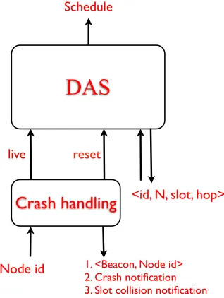
ActionsWe now present the actions of the modular algorithm. It is modular in the sense that the crash handling aspect is separate from the data aggregation scheduling algorithm (see Figure 3).
DAS
Crash handling
Schedule
1. <Beacon, Node id> 2. Crash notification 3. Slot collision notification
<id, N, slot, hop>
Node id
[image:16.612.231.390.210.421.2]reset live
Figure 3: The Modular Fault-tolerant DAS Algorithm of Figure 2
·Crash handlingFour actions are involved in the crash handling part:
1. neighbourS: This action is enabled everyλtime units, where nodes exchange “I am alive” message beacons with only
their id attached.
2. neighbourC: In this action, nodes collect the ids of those neighbours in a given round that send the “I am alive” messages.
3. check: In this action, a processjchecks whether his elected parent is still alive. If not, nodejresets its slot, hop and
parent variables, and broadcasts acrashmessage.
4. reset: When a nodej receives a crashmessage from a nodei, it checks if the message is relevant by checking if i
is his parent. If it is, thenj resets its node (as its slot is no longer weakly proper), and forwards thecrashmessage.
Thecrashmessage is forwarded so that every node that is affected by the crash, i.e., those that are affected by the path
disappearing, then these nodes can select a new parent.
·DAS handlingThe following actions are those that handle the DAS problem:
1. dissem: In this action, the process disseminates slot information. If the process is the sink, then it sends network
2. receive: With this action, nodes collect information about its 2-hop neighbourhood. This is so to avoid nodes in a 2-hop
neighbourhood to share the same slot, i.e., to avoid slot collision.
3. resolve: In this action, when a set of nodes is notified of a slot collision, the relevant nodes recompute their slot values
based on the rank of their respective id in the attached collision set.
4. check: In this action, nodes that have their slot/hop/parent values set will check whether their parents are still up. If not,
a crash message is broadcast. Next, a processjwill check if its slot is colliding with that of other nodes in its 2-hop
neighbourhood. If yes, acollisionmessage is broadcast. Else, a processjcollects values about its 2-hop neighbourhood
and sets its slot/hop/parent variables by choosing the smallest hop, and having as a parent a node with the smallest hop.
Then the slot is chosen according to the parent chosen.
The program contains two “waves”: (i) a slot dissemination wave (DAS handling) and (ii) a crash notification wave (crash
handling). Because a slot dissemination wave may be well underway when a crash happens, to minimise the number of
nodes that have to reset their slots, we attempt to “slow down” the slot dissemination wave, while “speeding up” the crash
notification wave. A similar idea was used in [8] in relation of tracking in WSNs, where erroneous information is overwritten
via a “slowing down” process. In [8], the erroneous information is due to transient faults corrupting the state of the program.
In this paper, the erroneous information is indirectly created through the node crashes.
The program works as follows: When the slot wave timer times out, each node sends the following information:hj, J, slot, hopi
(i.e., its id, its neighbourhood, its slot number, its hop number) (actiondissem). The sink sends a similar message with
analo-gous information (actiondissem). Nodejcollects all the messages received (actionreceive). It calculates a slot based on the
shortest path to the sink using the hop values collected (actioncheck). There can be slot collisions between nodes in the same
collision group. However, these are eventually resolved (actionresolve).
On the other hand, when thebeacontimer expires (actionNeighbourS), nodes send “I am alive” messages, and any crash
information collected by a node is forwarded to its children (actionsneighbourC,checkandreset). The children reset their
slot (since the path is no longer available), and inform their children about the crash (actionreset). This process is iterative.
The idea then is to (i) detect crash failures fast enough (i.e., reduce detection latency), and (ii) propagate crash information
fast enough so that the slot wave can be caught, thereby reducing the number of nodes requiring a reset. In our program, by
setting a low value ofλ(fast detection) and by forwardingcrashnotification instantly, and a high value ofδ(the slot wave is
“slowed down”), one can expect the number of nodes to reset their slots to be reduced.
6.2. Proof of Correctness
We now prove the correctness of the algorithm.
Lemma 1 (Correctness of DAS Handling). Given a network G = (V, E), where every node has at leastf + 1disjoint paths to the sink, wheref is a system parameter. Eventually, all nodesn ∈ (V \ {S})are assigned a weakly proper and
non-colliding slot.
Proof:
We prove this by induction over thehopvalue.
which is trivially weakly proper forG. The slots are also non-colliding forGas all nodes have unique ids, making their rank
in the sink’s neighbourhood unique. Hence, no two nodes in the 2-hop neighbourhood will have the same slot.
hop = kWe assume that all nodes at1≤hop≤khave weakly proper and non-colliding slots forG.
Induction HypothesisAll nodes at1≤hop≤k+ 1will eventually have weakly proper and non-colliding slots forG. When the wavetimer times out, ∀n ∈ V ·n.hop = k, ndisseminates hn, N \ {parent}, n.slot, ki. When a node
j in the 1-hop neighbourhood of node nat hop = k+ 1is not set, then, in action check, node j will choose j.slot =
n.slot−rank(j, N)< n.slot. If there is any slot collision with another nodel, i.e.,l.slot=j.slot, then, in actionresolve,
the value ofj.slotorl.slotgets smallerm meaning thatj.slot < n.slot. Hence, processjhas a weakly proper slot forG. If
the slot is not a non-colliding one, the nodes sharing the same slot will reduce the value of their slots by two different numbers
(actionresolve), hencejwill eventually obtain a non-colliding slot. On the other hand, ifn.slotcollided with another node,
then ifnreduces it slot such that its childrens’ slots are affected, then the children will choose again to ensure weakly proper
property. The weakly proper slot property is maintained during slot collision resolution as the slot values of colliding nodes
are reduced. The non-colliding property is eventually guaranteed through the actionresolve
Since nodes athop= 1have weakly proper and non-colliding slots and from the induction hypothesis, we conclude that
all nodes at1≤hop≤DGwill have weakly proper and non-colliding slots forG.
Lemma 2 (Correctness of crash handling ofd-local algorithm). Given a networkG = (V, E), where every node has at leastf + 1disjoint paths to the sink, and a fault modelF where up tof crash failures can occur. Then, only the nodes that
have the crashed nodes on their path to the sink will reset their slot/hop/parent values.
Proof
When a nodenis detected to have crashed by nodej such thatj.parent=n(through actionsneighbourS, neighbourC,
check), acrashmessage is sent by j. When a child ofj receives the notification, it resets its state in actionreset, and
re-broadcasts thecrashmessage. Only children of nodes that are resetting that will reset, until a node is reached that has not yet
set its slot/parent/hop values.
Lemma 3 (Crash recovery ofd-local algorithm). Given a networkG= (V, E), where every node has at leastf+ 1disjoint paths to the sink, and a fault modelF where up tof crash failures can occur. All nodes that have had their slots reset will
eventually be assigned new weakly proper and non-colliding slots.
Proof
After a node resets its state, it continues to collect neighbourhood information (actionsdissem, receive), as there is at least
one path still active. Using actionscheck and resolve, it eventually assigns itself a weakly proper and non-colliding slot.
Theorem 5 (Correctness ofd-local algorithm). Given a networkG= (V, E), where every node has at leastf + 1disjoint
paths to the sink, and a fault model where up tofcrash failures can occur. Then, the program of Figure 2 solves the stabilising
weak data aggregation scheduling problem.
Now, we present a result that shows that the algorithm of Figure 2 can achieve efficient stabilization. In fact, the algorithm
of Figure 2, thoughd-local, can be made to have a near-constant recovery overhead, under appropriate parameterization.
To show this, we define the notion ofperturbation areaas follows:
Definition 9 (Perturbation area). Given a networkG = (V, E)where every node has at leastf + 1disjoint paths to the
sink, and a fault modelF where up tof crashes can occur. Theperturbation sizeis the number of nodes in theF-affected
area.
From Definition 2, an affected area of a graphGis a subgraph ofGwhere all the nodes in the subgraph will have to change
their state. In the proposed algorithm, all the affected nodes (those in the affected area) will change their slot values to⊥.
Theorem 6 (Bounded perturbation area). Given a networkG= (V, E), where every node has at leastf+ 1disjoint paths to the sink, and a fault model where up tof crash failures can occur. Then, the program of Figure 2 solves stabilizing weak
data aggregation scheduling with a perturbation size of O(∆ λ δ G).
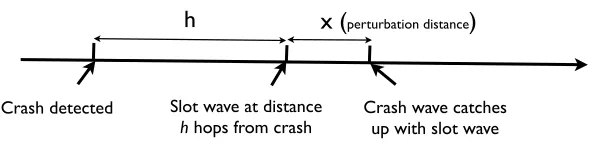
Crash detected Slot wave at distance
h hops from crash Crash wave catches up with slot wave
[image:19.612.143.439.435.510.2]h
x (
perturbation distance)
Figure 4: State of protocol when a crash is detected.
Proof
Assume a nodencrashes and assume that the slot wave is at a distancehhops away (i.e., the latest nodemto choose its
slot based onn(nis an ancestor ofm) ishhops away fromn- see Figure 4). In the time the crash information propagates,
the slot information, atwaveperiodδ, propagates too over a distancex(which we call perturbation distance).
Let the time it takes for the crash information to catch up with the slot wave be denoted byτ, and let the crash propagation
speed behops per second.
Then, we have the following:
τ=λ+x+h
This means that inτtime units, the wave will traveldτ
δe=xhops. At the same time, a child ofnneedsλtime units to
detect the crash and then the crash wave will travelh+xhops (to catch up with the slot wave). The time taken will be h+x .
Simplifying the equation, we have
x=λ+h
δ−1
Sinceis likely to be big, then
x≈ λ
δ
Since the degree of the graphGis∆G, then the perturbation area isO(∆ λ δ
G).
Now, given that the objective is to minimisex, ifδ =λ, then the size of the perturbation area may be big, depending on
howcompares withδ. However, by settingδto be much larger thanλ(and allowingto be large - note that this parameter
is outside the control of the protocol and simulation) (i.e., slowing down the “slot” wave), the size of the affected area can be
bounded, and approachesO(1)- with the result that the algorithm approaches2-local stabilizing.
6.3. Performance Analysis and Comparison
In this section, we present a analysis of the performance of our algorithm and we subsequently make a comparison with
an algorithm, presented in [28], which is sufficiently close to that presented in the paper.
Performance Analysis: Time and Message Complexities, Energy Efficiency and Latency
The time (in terms of rounds) to execute the algorithm is O(DG) as all nodes at a given hop count make decisions
concur-rently and there is a maximum ofDG hops inG. For the communication cost, which is measured in terms of the number of
messages, the following is taken into account: (i) number of slot waves, (ii) number of beacons and (iii) number of collision
messages. The number of slot waves isO(ηGDG), since nodes at hop = 1 will transmit forDGrounds. The number of beacons
isO(ΓDG), since the number of beacons is a multiple of the number of slot waves. The number of collision messages to be
generated has the same complexity, giving the communication cost a complexity ofO(ΓDG)(orO(ΓlogΓ)).
The latency of our algorithm isO(DG(∆G+αG)), whereαG is the maximum size of a collision group in the network.
The smallest slot for nodes at hop = 1 is bounded byΓ−∆G−αG. The smallest slot in the network will then be bounded by
Γ−(∆G+αG)DG, giving a latency bound of(∆G+αG)DG.
Performance Comparison
We compare our work with that presented in [28], which is the closest to the one we present here. Both the time and
message complexities of our algorithm is similar to those of [28], though the algorithm in [28] is not fault-tolerant. The
algorithm in [28] is later adapted to make it tolerate crashes, however no performance analysis is available for comparison to
include beacons and adaptivity messages. Energy-efficiency is closely related to the number of message transmissions and,
thus, our algorithm is similar in efficiency to that of [28].
The latency of the algorithm in [28] isO(24DG+ 6∆G+ 16), compared toO(∆G+αG)DGfor that presented here. The
7. Experiments: Setup and Results
In this section, we first present the simulation setup we use to test the performance of our algorithm, and the results are
presented subsequently.
7.1. Simulation Setup
For our simulations, we used JProwler, a Java-based, event-driven simulator for wireless sensor networks [13]. JProwler
simulates the transmission/propagation/reception delays of Mica2 motes and the operation of the MAC-layer. We used two
network topologies: (i) a grid topology, and (ii) a ring topology. In both cases, a node is equidistant from its neighbours. The
signal strength is set such that the degree of a node in the network is between 2 (for rings left and right neighbours) and 4
(for grids, top, bottom, left and right neighbours). We implemented the whole algorithm, and crashed specific nodes during
execution.
Network setupOur implementation of the protocol (Figure 2) for handling crash failures when setting up a WSN under
JProwler is a per node, message-passing distributed program. Our experimental data consists of running our simulations on
(i)g×ggrids, whereg= 11,15,21,25, and (ii) rings of size4g−4, whereg∈ {11,15,21,25}.
When inducing crash failures, we have to choose (i) which node to crash, and (ii) the time at which to crash the node. Note
that only one node can be crashed since the grids and rings we generated for our simulations only offer two disjoint paths to
the sink.
Choosing Node to CrashIn our simulations, we choose the set of all nodes that are within4hops of the sink, which we denote byΩ. The nodes inΩare those that we crash. The reason for choosing these nodes is to allow “maximum” impact on
the rest of the network.
Crash FailuresIn our simulation, we crash one nodenfrom theΩ(i.e., we crash a noden ∈Ω) at certain times after the nodenhas had its values set, and these times are 5, 10, 15, 20 and 25 seconds. Specifically, one crash scenario consists of (i)
choosing a crash timeτ∈ {5,10,15,20,25s}, and (ii) choosing one noden∈Ωthat is within 4 hops from the sink that will
be crashed.
Data Collection and MetricsEach crash scenario (choosing a node to crash and a crash time) is executed 20 times. We then take the average number of nodes reset from all of these runs. These simulations are then repeated for various settings of
network size,δandλ(from the protocol). We analyse the data and focus on the average number of resets (actionreset) when
crash failures occur. This metric captures the locality property of the algorithm.
7.2. Simulation Results
In this section, we present the results detailing the performance of the protocol presented in Figure 2. We focus on the
number of resets, which captures the size of the perturbation area (hence the locality property).
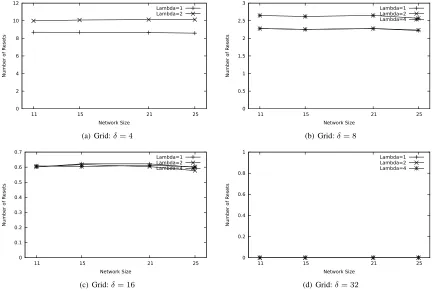
7.2.1. Grid Networks: Number of Resets
As can be observed from Figure 5, as δ increases, then the number of resets decreases. Specifically, as λδ becomes
smaller, the size of the perturbation area decreases. This is due to the fact that the slot wave is “slowed” down a lot, the crash
information wave has a greater chance of catching up with the slot wave. Also, aλincreases, detection of crashes takes more
time, giving the chance for the slot wave to propagate further, thereby causing an increase in the number of resets. Thus, from
our observation, a low value ofλand a high value ofδwill cause a very small number of resets. In fact, in Figure 5(d), we
0 2 4 6 8 10 12
11 15 21 25
Number of R
esets
Network Size
Lambda=1 Lambda=2
(a) Grid:δ= 4
0 0.5 1 1.5 2 2.5 3
11 15 21 25
Number of R
esets
Network Size
Lambda=1 Lambda=2 Lambda=4
(b) Grid:δ= 8
0 0.1 0.2 0.3 0.4 0.5 0.6 0.7
11 15 21 25
Number of R
esets
Network Size
Lambda=1 Lambda=2 Lambda=4
(c) Grid:δ= 16
0 0.2 0.4 0.6 0.8 1
11 15 21 25
Number of R
esets
Network Size
Lambda=1 Lambda=2 Lambda=4
[image:22.612.87.524.60.351.2](d) Grid:δ= 32
Figure 5: Grid: Number of Resets vs Network Size
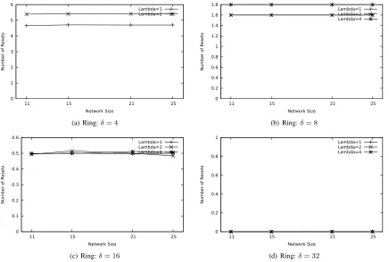
7.2.2. Ring Networks: Number of Resets
As can be observed from Figure 6, asδincreases, then the number of resets decreases. This is again due to the fact that
the slot wave is “slowed” down a lot, the crash information wave has a greater chance of catching up the slot wave. Also, aλ
increases, detection of crashes takes more time, giving the chance for the slot wave to propagate further, thereby causing an
increase in the number of resets. Thus, from our observation, a low value ofλand a high value ofδwill cause a very small
number of resets.
Comparing Figures 5 and 6, it can be observed that the number of resets is greater in grid networks than in ring networks.
This is due to the fact that, in grid networks, a node has a higher number of neighbours than in ring networks.
7.2.3. Grid Networks: Completion Latency
For the sake of completeness, we present some results that show the modularity of our proposed algorithm, in that the
DAS aspect completes in parallel with the correction aspect (for stabilisation). From Figure 7, we observe that all the graphs
are almost identical. Hence, irrespective of the size of the network, the completion time is similar, indicating that the DAS
completes irrespective of the time and location of the crash. This captures the modularity of our algorithmm.
7.3. Experimental Results
To assess whether the execution of the protocol is as predicted by our mathematical analysis, we also conducted a
de-ployment on a small testbed of10CM5000 sensor motes, which are based on the TelosB platform. We perform an indoor
deployment, setting the transmission power of each node to a very low level 2. Our implementation of the protocol requires
0 1 2 3 4 5 6
11 15 21 25
Number of R
esets
Network Size
Lambda=1 Lambda=2
(a) Ring:δ= 4
0 0.2 0.4 0.6 0.8 1 1.2 1.4 1.6 1.8
11 15 21 25
Number of R
esets
Network Size
Lambda=1 Lambda=2 Lambda=4
(b) Ring:δ= 8
0 0.1 0.2 0.3 0.4 0.5 0.6
11 15 21 25
Number of R
esets
Network Size
Lambda=1 Lambda=2 Lambda=4
(c) Ring:δ= 16
0 0.2 0.4 0.6 0.8 1
11 15 21 25
Number of R
esets
Network Size
Lambda=1 Lambda=2 Lambda=4
[image:23.612.88.524.58.352.2](d) Ring:δ= 32
Figure 6: Ring: Number of Resets vs Network Size
The network deployed is as depicted in Figure 8. As in the simulations, we are interested in the number of resets, where
a low number will prove the locality of the protocol. We set the beacon period toλ = {5s,7s}, and the slot wave period
δ = {10s,20s,40s,14s,28s,56s}, i.e.,δ = {2,4,8}λ. We first allowed the system to run for 5 beacon periods to allow
nodes to gather their neighbourhoods. In every run, node 1 was crashed a random time after it has broadcast its state. The
reason for crashing node 1 is that it allows for maximum impact to be observed and the reason for crashing the node after it
broadcasts is to observe how the state of the children are affected. This combination allows for a “worst-case” situation. Each
run was repeated 5 times and, for each run, the number of resets is counted, and the average taken. For each value of beacon
(and wave period) considered, the number of resets is 2 (hence the average is 2), where nodes 3 and 4 would reset due to their
parent, i.e., 1, crashing. This confirms the locality property of the protocol.
8. Related Work
In this section, we survey the area of data aggregation scheduling (e.g., [26]) and convergecast algorithms (e.g., [23]).
Since traditional convergecast is very different to data aggregation convergecast, we focus on works about data aggregation
scheduling. Most works on DAS or convergecast have focused on optimizing some metric, for example latency or throughput.
There exists both centralised and distributed algorithms for DAS.
Centralized algorithmsA number of centralised algorithms [26, 24, 7, 22] have been proposed in the literature where the goals was to optimize some objectives, e.g., latency [26], aggregation time [7], concurrency [22]. Further, none of these
algorithms are fault-tolerant, in contrast to the work presented here.
0 10 20 30 40 50 60 70
11 15 21 25
Maximum Latency
Network Size
Lambda=1 Lambda=2
(a) Ring:δ= 4
0 10 20 30 40 50 60 70
11 15 21 25
Maximum Latency
Network Size
Lambda=1 Lambda=2 Lambda=4
(b) Ring:δ= 8
0 10 20 30 40 50 60 70
11 15 21 25
Maximum Latency
Network Size
Lambda=1 Lambda=2 Lambda=4
(c) Ring:δ= 16
0 10 20 30 40 50 60 70
11 15 21 25
Maximum Latency
Network Size
Lambda=1 Lambda=2 Lambda=4
[image:24.612.89.524.57.345.2](d) Ring:δ= 32
Figure 7: Grid: Completion Time vs Network Size
ever, none of the above work is known to tolerate any types of failures such as crash or transient faults. The approach presented
in [28] presents an adaptive strategy for their DAS in the presence of crash failure. To achieve this transformation, they
intro-duce beacons to detect node crashes and nodes execute steps to obtain new parents. The authors of [28] claim fault locality of
their algorithm, though there is no proof of correctness of the property. Further, the authors also claim that, in the presence of
a number of nodes failing, they re-execute their algorithm again, in contrast to our approach here.
To the best of our knowledge, the only known works that focuses on fault tolerant DAS/convergecast are those by
Jhumka [18] and by Arumugam and Kulkarni [19]. The work presented in [18] focused on DAS in the presence of a
sin-gle crash failure. In this work, we extend the work of [18] by (i) generalizing the result to deal withf faults, (ii) we propose
an algorithm that work on general networks, and (iii) we provide simulation results to show the efficiency of the proposed
algorithm. In [19], the authors develop a stabilising convergecast algorithm. However, the authors of [19] made assumptions
which we do not, such as (i) each node knows their exact location in the network, (ii) the network is a grid, though they
pro-vided hints as to how to relax these constraints, and (iii) the fault model is one that corrupts the state of the network, whereas
we assume crash failures in this work.
The area of graph colouring is closely related to the area under investigation here, and have been extensively studied
before. The problem of graph colouring involves assigning a set of colours to nodes or links under various constraints. For
example, the authors of [4] showed how to use 2-distance colouring to obtain a TDMA schedule for a wireless sensor network,
where 2-distance colouring is required so that slots are assigned in such a way to avoid collisions between nodes. However,
most of the work in graph colouring may not be easily applied to our problem here, since DAS requires an ordering on the
2
1
4
6
8
9
7
5
[image:25.612.169.451.99.211.2]3
0
Figure 8: Network used in deployment, with node 0 being the sink.
Finally, since our approach involves developing a tree structure, the seminal work by Maddenet al.[14] on aggregation
service during queries adopted a similar approach. However, the tree structure in [14] is continuously maintained by the root
(sink), by periodically broadcasting relevant information to make the structure tolerant to node failures or topology changes.
Thus, maintaining the tree structure involves the whole network (i.e., O(N), where N is the network size) and is, thus,
not energy-efficient. This maintenance is also performed even though there may not have been any change in the network
topology.
In other related work regarding fault tolerance in wireless ad hoc networks, we note the comparison-based techniques
developed in [11, 12] for detecting faulty nodes through an assignment of tasks to nodes, though the types of faults assumed
is different from this work. The area of self stabilisation [10] has been widely applied to wireless sensor networks to tolerate
transient faults, e.g., [17, 3, 8].
9. Discussion
In this section, we will discuss some of the issues raised by our work and the design decisions made in our work.
The first observation is that the nodes periodically broadcast their state information, which is not optimal in terms of the
number of messages. We emphasise that the objective of the paper is to conduct a study on DAS in presence of crash failures,
and not on protocol optimisations. However, the reason for periodic broadcasts is for the need to detect slot collisions. Since
a node can haveO(∆G)slot collisions, and with a diameter ofDG, the number of broadcasts can be quite high. Several
optimisations are possible to reduce the number of messages transmitted. For example, the protocol can be optimised by
having nodes broadcast a special message only when they are resetting their state. This will enable potential new parents to
send their state information to those nodes with reset state only during crashes. Another possible optimisation is to have slot
information about the 2-hop neighbourhood piggy-backed onto messages, such that whenever a node is choosing a slot, it has
all the relevant slot information readily available.