Weakly Supervised Part of Speech Tagging for Morphologically Rich, Resource Scarce Languages

Weakly Supervised Part-of-Speech Tagging for Morphologically-Rich,

Resource-Scarce Languages

Kazi Saidul Hasan and Vincent Ng Human Language Technology Research Institute

University of Texas at Dallas Richardson, TX 75083-0688

{saidul,vince}@hlt.utdallas.edu

Abstract

This paper examines unsupervised ap-proaches to part-of-speech (POS) tagging for morphologically-rich, resource-scarce languages, with an emphasis on Goldwa-ter and Griffiths’s (2007) fully-Bayesian approach originally developed for En-glish POS tagging. We argue that ex-isting unsupervised POS taggers unreal-istically assume as input a perfect POS lexicon, and consequently, we propose a weakly supervised fully-Bayesian ap-proach to POS tagging, which relaxes the unrealistic assumption by automatically acquiring the lexicon from a small amount of POS-tagged data. Since such relaxation comes at the expense of a drop in tag-ging accuracy, we propose two extensions to the Bayesian framework and demon-strate that they are effective in improv-ing a fully-Bayesian POS tagger for Ben-gali, our representative morphologically-rich, resource-scarce language.

1 Introduction

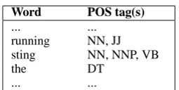
Unsupervised POS tagging requires neither man-ual encoding of tagging heuristics nor the avail-ability of data labeled with POS information. Rather, an unsupervised POS tagger operates by only assuming as input a POS lexicon, which con-sists of a list of possible POS tags for each word. As we can see from the partial POS lexicon for English in Figure 1, “the” is unambiguous with re-spect to POS tagging, since it can only be a deter-miner (DT), whereas “sting” is ambiguous, since it can be a common noun (NN), a proper noun (NNP) or a verb (VB). In other words, the lexi-con imposes lexi-constraints on the possible POS tags

Word POS tag(s)

... ...

running NN, JJ

sting NN, NNP, VB

the DT

... ...

Figure 1: A partial lexicon for English

of each word, and such constraints are then used by an unsupervised tagger to label a new sentence. Conceivably, tagging accuracy decreases with the increase in ambiguity: unambiguous words such as “the” will always be tagged correctly; on the other hand, unseen words (or words not present in the POS lexicon) are among the most ambigu-ous words, since they are not constrained at all and therefore can receive any of the POS tags. Hence, unsupervised POS tagging can present sig-nificant challenges to natural language processing researchers, especially when a large fraction of the words are ambiguous. Nevertheless, the de-velopment of unsupervised taggers potentially al-lows POS tagging technologies to be applied to a substantially larger number of natural languages, most of which are resource-scarce and, in particu-lar, have little or no POS-tagged data.

demonstrated promising results, it is important to note that they are typically evaluated by assuming the availability of a perfect POS lexicon. This as-sumption, however, is fairly unrealistic in practice, as a perfect POS lexicon can only be constructed by having a linguist manually label each word in a language with its possible POS tags.1 In other words, the labor-intensive POS lexicon construc-tion process renders unsupervised POS taggers a lot less unsupervised than they appear. To make these unsupervised taggers practical, one could at-tempt to automatically construct a POS lexicon, a task commonly known as POS induction. How-ever, POS induction is by no means an easy task, and it is not clear how well unsupervised POS tag-gers work when used in combination with an au-tomatically constructed POS lexicon.

The goals of this paper are three-fold. First, motivated by the successes of unsupervised ap-proaches to English POS tagging, we aim to inves-tigate whether such approaches, especially G&G’s fully-Bayesian approach, can deliver similar per-formance for Bengali, our representative resource-scarce language. Second, to relax the unrealis-tic assumption of employing a perfect lexicon as in existing unsupervised POS taggers, we propose a weakly supervised fully-Bayesian approach to POS tagging, where we automatically construct a POS lexicon from a small amount of POS-tagged data. Hence, unlike a perfect POS lexicon, our au-tomatically constructed lexicon is necessarily

in-complete, yielding a large number of words that

are completely ambiguous. The high ambiguity rate inherent in our weakly supervised approach substantially complicates the POS tagging pro-cess. Consequently, our third goal of this paper is to propose two potentially performance-enhancing extensions to G&G’s Bayesian POS tagging ap-proach, which exploit morphology and techniques successfully used in supervised POS tagging.

The rest of the paper is organized as follows. Section 2 presents related work on unsupervised approaches to POS tagging. Section 3 gives an introduction to G&G’s fully-Bayesian approach to unsupervised POS tagging. In Section 4, we describe our two extensions to G&G’s approach. Section 5 presents experimental results on Bengali POS tagging, focusing on evaluating the

effective-1_{When evaluating an unsupervised POS tagger,}

re-searchers typically construct a pseudo-perfect POS lexicon by collecting the possible POS tags of a word directly from the corpus on which the tagger is to be evaluated.

ness of our two extensions in improving G&G’s approach. Finally, we conclude in Section 6.

2 Related Work

3 A Fully Bayesian Approach

3.1 Motivation

As mentioned in the introduction, the most com-mon approach to unsupervised POS tagging is to train an HMM on an unannotated corpus using the Baum-Welch algorithm so that the likelihood of the corpus is maximized. To understand what the HMM parameters are, let us revisit how an HMM simultaneously generates an output sequence w

= (w0, w1, ..., wn)and the associated hidden state sequence t= (t0, t1, ..., tn). In the context of POS tagging, each state of the HMM corresponds to a POS tag, the output sequence w is the given word sequence, and the hidden state sequence t is the associated POS tag sequence. To generate w and

t, the HMM begins by guessing a statet0and then

emitting w0 from t0 according to a state-specific output distribution over word tokens. After that, we move to the next state t1, the choice of which is based on t0’s transition distribution, and emit w1according tot1’s output distribution. This gen-eration process repeats until the end of the word sequence is reached. In other words, the parame-ters of an HMM,θ, are composed of a set of state-specific (1) output distributions (over word tokens) and (2) transition distributions, both of which can be learned using the EM algorithm. Once learning is complete, we can use the resulting set of param-eters to find the most likely hidden state sequence given a word sequence using the Viterbi algorithm. Nevertheless, EM sometimes fails to find good parameter values.2 _{The reason is that EM tries to}

assign roughly the same number of word tokens to each of the hidden states (Johnson, 2007). In prac-tice, however, the distribution of word tokens to POS tags is highly skewed (i.e., some POS cate-gories are more populated with tokens than oth-ers). This motivates a fully-Bayesian approach, which, rather than committing to a particular set of parameter values as in an EM-based approach, integrates over all possible values of θand, most importantly, allows the use of priors to favor the learning of the skewed distributions, through the use of the termP(θ|w)in the following equation:

P(t|w) =

Z

P(t|w, θ)P(θ|w)dθ (1)

The question, then, is: which priors onθwould allow the acquisition of skewed distributions? To

2_{When given good parameter initializations, however, EM}

can find good parameter values for an HMM-based POS tag-ger. See Goldberg et al. (2008) for details.

answer this question, recall that in POS tagging,θ is composed of a set of tag transition distributions and output distributions. Each such distribution is a multinomial (i.e., each trial produces exactly one of some finite number of possible outcomes). For a multinomial withKoutcomes, aK-dimensional Dirichlet distribution, which is conjugate to the multinomial, is a natural choice of prior. For sim-plicity, we assume that a distribution inθis drawn from a symmetric Dirichlet with a certain hyper-parameter (see Teh et al. (2006) for details).

The value of a hyperparameter, α, affects the skewness of the resulting distribution, as it as-signs different probabilities to different distribu-tions. For instance, when α < 1, higher proba-bilities are assigned to sparse multinomials (i.e., multinomials in which only a few entries are non-zero). Intuitively, the tag transition distributions and the output distributions in an HMM-based POS tagger are sparse multinomials. As a re-sult, it is logical to choose a Dirichlet prior with α < 1. By integrating over all possible param-eter values, the probability that i-th outcome, yi, takes the value k, given the previous i−1 out-comes y₋i= (y1, y2, ..., yi−1), is

P(k|y−i, α) = Z

P(k|θ)P(θ|y−i, α)dθ(2)

= nk+α

i−1 +Kα (3)

where nk is the frequency of k in y−i. See

MacKay and Peto (1995) for the derivation.

3.2 Model

Our baseline POS tagging model is a standard tri-gram HMM with tag transition distributions and output distributions, each of which is a sparse multinomial that is learned by applying a symmet-ric Disymmet-richlet prior:

ti |ti−1, ti−2, τ

(ti

−1,ti−2) ∼Mult(τ(ti−1,ti−2)) wi |ti, ω(ti) ∼Mult(ω(ti)) τ(ti

−1,ti−2)|α ∼Dirichlet(α) ω(ti)_{|β ∼Dirichlet(β)}

wherewiandtidenote thei-th word and tag. With a tagset of sizeT (including a special tag used as sentence delimiter), each of the tag transition dis-tributions hasT components. For the output sym-bols, each of theω(ti)

hasWti components, where

From the closed form in Equation 3, given pre-vious outcomes, we can compute the tag transition and output probabilities of the model as follows:

P(ti|t−i, α) =

n_(ti

−2,ti−1,ti)+α n_(ti

−2,ti−1)+T α

(4)

P(wi|ti,t−i,w−i, β) =

n_(ti,wi)+β

nti+Wtiβ (5)

where n_(ti

−2,ti−1,ti) and n(ti,wi) are the

frequen-cies of observing the tag trigram (ti−2, ti−1, ti)

and the tag-word pair(ti, wi), respectively. These counts are taken from the i−1 tags and words generated previously. The inference procedure de-scribed next exploits the property that trigrams (and outputs) are exchangeable; that is, the prob-ability of a set of trigrams (and outputs) does not depend on the order in which it was generated.

3.3 Inference Procedure

We perform inference using Gibbs sampling (Ge-man and Ge(Ge-man, 1984), using the following pos-terior distribution to generate samples:

P(t|w, α, β)∝P(w|t, β)P(t|α)

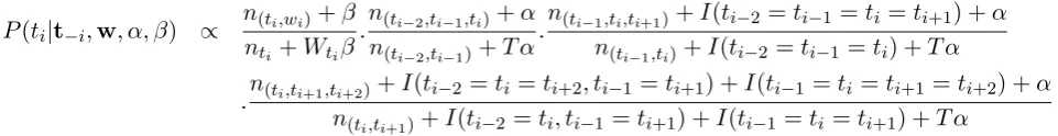
Starting with a random assignment of a POS tag to each word (subject to the constraints in the POS lexicon), we resample each POS tag, ti, accord-ing to the conditional distribution shown in Figure 2. Note that the current counts of other trigrams and outputs can be used as “previous” observa-tions due to the property of exchangeability.

Following G&G, we use simulated annealing to find the MAP tag sequence. The temperature

de-creases by a factor ofexp(log(

θ₂ θ₁)

N−1 )after each

iter-ation, whereθ1 is the initial temperature andθ2 is the temperature afterN sampling iterations.

4 Two Extensions

In this section, we present two extensions to G&G’s fully-Bayesian framework to unsupervised POS tagging, namely, induced suffix emission and discriminative prediction.

4.1 Induced Suffix Emission

For morphologically-rich languages like Bengali, a lot of grammatical information (e.g., POS) is ex-pressed via suffixes. In fact, several approaches to unsupervised POS induction for morphologically-rich languages have exploited the observation that some suffixes can only be associated with a small

number of POS tags (e.g., Clark (2003), Dasgupta and Ng (2007)). To exploit suffixes in HMM-based POS tagging, one can (1) convert the word-based POS lexicon to a suffix-word-based POS lexicon, which lists the possible POS tags for each suffix; and then (2) have the HMM emit suffixes rather than words, subject to the constraints in the suffix-based POS lexicon. Such a suffix-suffix-based HMM, however, may suffer from over-generalization. To prevent over-generalization and at the same time exploit suffixes, we propose as our first exten-sion to G&G’s framework a hybrid approach to word/suffix emission: a word is emitted if it is present in the word-based POS lexicon; otherwise, its suffix is emitted. In other words, our approach imposes suffix-based constraints on the tagging of words that are unseen w.r.t. the word-based POS lexicon. Below we show how to induce the suffix of a word and create the suffix-based POS lexicon.

Inducing suffixes To induce suffixes, we rely on

Keshava and Pitler’s (2006) method. Assume that (1)V is a vocabulary (i.e., a set of distinct words) extracted from a large, unannotated corpus, (2)C₁ andC2are two character sequences, and (3)C1C2 is the concatenation of C1 and C2. If C1C2 and C₁are found inV, we extractC₂as a suffix.

However, this unsupervised suffix induction method is arguably overly simplistic and hence many of the induced affixes could be spurious. To identify suffixes that are likely to be correct, we employ a simple procedure: we (1) score each suf-fix by multiplying its frequency (i.e., the number of distinct words in V to which each suffix at-taches) and its length3, and (2) select only those whose score is above a certain threshold. In our experiments, we set this threshold to 50, and gen-erate our vocabulary from five years of articles taken from the Bengali newspaper Prothom Alo. This enables us to induce 975 suffixes.

Constructing a suffix-based POS lexicon

Next, we construct a suffix-based POS lexicon. For each word w in the original word-based POS lexicon, we (1) use the induced suffix list obtained in the previous step to identify the longest-matching suffix ofw, and then (2) assign all the POS tags associated withwto this suffix.

Incorporating suffix-based output distributions Finally, we extend our trigram model by

introduc-3_{The dependence on frequency and length is motivated by}

P(ti|t−i,w, α, β) ∝

n_(ti,wi)+β

nti +Wtiβ

.n(ti

−2,ti−1,ti)+α n_(ti

−2,ti−1)+T α .n(ti

−1,ti,ti+1)+I(ti−2=ti−1 =ti =ti+1) +α n_(ti

−1,ti)+I(ti−2=ti−1=ti) +T α

.n(ti,ti+1,ti+2)+I(ti−2 =ti=ti+2, ti−1 =ti+1) +I(ti−1=ti =ti+1=ti+2) +α

n_(ti,ti+1)+I(ti−2=ti, ti−1 =ti+1) +I(ti−1 =ti =ti+1) +T α

Figure 2: The sampling distribution forti (taken directly from Goldwater and Griffiths (2007)). Allnx values are computed from the current values of all tags except for ti. Here, I(arg) is a function that returns 1 ifargis true and 0 otherwise, andt−i refers to the current values of all tags except forti.

ing a state-specific probability distribution over in-duced suffixes. Specifically, if the current word is present in the word-based POS lexicon, or if we cannot find any suffix for the word using the in-duced suffix list, then we emit the word. Other-wise, we emit its suffix according to a suffix-based output distribution, which is drawn from a sym-metric Dirichlet with hyperparameterγ:

si|ti, σ(ti) ∼Mult(σ(ti)) σ(ti)_{|γ ∼Dirichlet(γ)}

where si denotes the induced suffix of the i-th word. The distribution, σ(ti)_{, hasS}

ticomponents, whereSti denotes the number of induced suffixes that can be emitted from the state corresponding to ti. We compute the induced suffix emission prob-abilities of the model as follows:

P(si|ti,t−i,s−i, γ) =

n(ti,si)+γ

nti+Stiγ

(6)

where n_(ti,si) is the frequency of observing the tag-suffix pair(ti, si).

This extension requires that we slightly modify the inference procedure. Specifically, if the cur-rent word is unseen (w.r.t. the word-based POS lexicon) and has a suffix (according to the induced suffix list), then we sample from a distribution that is almost identical to the one shown in Figure 2, except that we replace the first fraction (i.e., the fraction involving the emission counts) with the one shown in Equation (6). Otherwise, we simply sample from the distribution in Figure 2.

4.2 Discriminative Prediction

As mentioned in the introduction, the (word-based) POS lexicons used in existing approaches to unsupervised POS tagging were created some-what unrealistically by collecting the possible POS tags of a word directly from the corpus on which the tagger is to be evaluated. To make the

lexicon formation process more realistic, we pro-pose a weakly supervised approach to Bayesian POS tagging, in which we automatically create the word-based POS lexicon from a small set of POS-tagged sentences that is disjoint from the test data. Adopting a weakly supervised approach has an ad-ditional advantage: the presence of POS-tagged sentences makes it possible to exploit techniques developed for supervised POS tagging, which is the idea behind discriminative prediction, our sec-ond extension to G&G’s framework.

Given a small set of POS-tagged sentencesL, discriminative prediction uses the statistics col-lected from L to predict the POS of a word in a discriminative fashion whenever possible. More specifically, discriminative prediction relies on two simple ideas typically exploited by supervised POS tagging algorithms: (1) if the target word (i.e., the word whose POS tag is to be predicted) appears inL, we can label the word with its POS tag inL; and (2) if the target word does not appear inLbut its context does, we can use its context to predict its POS tag. In bigram and trigram POS taggers, the context of a word is represented us-ing the precedus-ing one or two words. Nevertheless, since Lis typically small in a weakly supervised setting, it is common for a target word not to sat-isfy any of the two conditions above. Hence, if it is not possible to predict a target word in a discrim-inative fashion (due to the limited size ofL), we resort to the sampling equation in Figure 2.

To incorporate the above discriminative deci-sion steps into G&G’s fully-Bayesian framework for POS tagging, the algorithm estimates three types of probability distributions from L. First, to capture context, it computes (1) a distribu-tion over the POS tags following a word bi-gram,(wi−2, wi−1), that appears inL[henceforth

D1(wi−2, wi−1)] and (2) a distribution over the

POS tags following a word unigram,wi−1, that

cap-Algorithm 1 cap-Algorithm for incorporating discrim-inative prediction

Input: wi: current word

wi

−1: previous word wi

−2: second previous word L: a set of POS-tagged sentences Output: Predicted tag,ti

1: ifwi∈Lthen

2: ti ←Tag drawn from the distribution ofwi’s

candi-date tags 3: else if(wi

−2, wi−1)∈Lthen

4: ti←Tag drawn from the distribution of the POS tags

following the word bigram(wi

−2, wi−1) 5: else ifwi

−1∈Lthen

6: ti←Tag drawn from the distribution of the POS tags

following the word unigramwi

−1 7: else

8: ti←Tag obtained using the sampling equation

9: end if

ture the fact that a word can have more than one POS tag, it also estimates a distribution over POS tags for each word wi that appears in L [hence-forthD3(wi)].

Implemented as a set of if-else clauses, the al-gorithm uses these three types of distributions to tag a target word, wi, in a discriminative manner. First, it checks whetherwiappears inL(line 1). If so, it tags wi according toD3(wi). Otherwise, it attempts to labelwibased on its context. Specifi-cally, if(wi−2, wi−1), the word bigram preceding

wi, appears inL(line 3), thenwiis tagged accord-ing toD1(wi−2, wi−1). Otherwise, it backs off to

a unigram distribution: ifwi−1, the word

preced-ing wi, appears in L (line 5), then wi is tagged according toD2(wi−1). Finally, if it is not

possi-ble to tag the word discriminatively (i.e., if all the above cases fail), it resorts to the sampling equa-tion (lines 7–8). We apply simulated annealing to all four cases in this iterative tagging procedure.

5 Evaluation

5.1 Experimental Setup

Corpus Our evaluation corpus is the one used

in the shared task of the IJCNLP-08 Workshop on NER for South and South East Asian Languages.4 Specifically, we use the portion of the Bengali dataset that is manually POS-tagged. IIIT Hy-derabad’s POS tagset5, which consists of 26 tags specifically developed for Indian languages, has been used to annotate the data. The corpus is com-posed of a training set and a test set with

approxi-4

The corpus is available from http://ltrc.iiit.ac.in/ner-ssea-08/index.cgi?topic=5.

5

http://shiva.iiit.ac.in/SPSAL2007/iiit tagset guidelines.pdf

mately 50K and 30K tokens, respectively. Impor-tantly, all our POS tagging results will be reported using only the test set; the training set will be used for lexicon construction, as we will see shortly.

Tagset We collapse the set of 26 POS tags into

15 tags. Specifically, while we retain the tags cor-responding to the major POS categories, we merge some of the infrequent tags designed to capture Indian language specific structure (e.g., reduplica-tion, echo words) into a category called OTHERS.

Hyperparameter settings Recall that our

tag-ger consists of three types of distributions — tag transition distributions, word-based output distri-butions, and suffix-based output distributions — drawn from a symmetric Dirichlet with α, β, and γ as the underlying hyperparameters, respec-tively. We automatically determine the values of these hyperparameters by (1) randomly initializ-ing them and (2) resamplinitializ-ing their values by usinitializ-ing a Metropolis-Hastings update (Gilks et al., 1996) at the end of each sampling iteration. Details of this update process can be found in G&G.

Inference Inference is performed by running a

Gibbs sampler for 5000 iterations. The initial tem-perature is set to 2.0, which is gradually lowered to 0.08 over the iterations. Owing to the random-ness involved in hyperparameter initialization, all reported results are averaged over three runs.

Lexicon construction methods To better

1 2 3 4 5 6 7 8 9 10 30

40 50 60 70 80 90

d

Accuracy (%)

(a) Lexicon 1

MLHMM BHMM BHMM+IS

1 2 3 4 5 6 7 8 9 10

30 35 40 45 50 55 60 65 70 75

d

Accuracy (%)

(b) Lexicon 2

MLHMM BHMM BHMM+IS

Figure 3: Accuracies of POS tagging models using (a) Lexicon 1 and (b) Lexicon 2

from 1 to 10 in our experiments. Any unseen (i.e., out-of-dictionary) word is ambiguous among the 15 possible tags. Not surprisingly, both ambigu-ity and the unseen word rate increase withd. For instance, the ambiguous token rate increases from 40.0% with 1.7 tags/token (d=1) to 77.7% with 8.1 tags/token (d=10). Similarly, the unseen word rate increases from 16% (d=2) to 46% (d=10). We will refer to this set of tag dictionaries as Lexicon 1.

The second method generates a set of relaxed lexicons, Lexicon 2, in essentially the same way as the first method, except that these lexicons in-clude only the words that appear at least dtimes in the training data. Importantly, the words that appear solely in the test data are not included in any of these relaxed POS lexicons. This makes Lexicon 2 a bit more realistic than Lexicon 1 in terms of the way they are constructed. As a result, in comparison to Lexicon 1, Lexicon 2 has a con-siderably higher ambiguous token rate and unseen word rate: its ambiguous token rate ranges from 64.3% with 5.3 tags/token (d=1) to 80.5% with 8.6 tags/token (d=10), and its unseen word rate ranges from 25% (d=1) to 50% (d=10).

The third method, arguably the most realistic among the three, is motivated by our proposed weakly supervised approach. In this method, we (1) form ten different datasets from the (labeled) training data of sizes 5K words, 10K words, . . ., 50K words, and then (2) create one POS lexicon from each datasetLby listing, for each wordwin L, all the tags associated withwinL. This set of tag dictionaries, which we will refer to as Lexicon

3, has an ambiguous token rate that ranges from

57.7% with 5.1 tags/token (50K) to 61.5% with 8.1 tags/token (5K), and an unseen word rate that ranges from 25% (50K) to 50% (5K).

5.2 Results and Discussion

5.2.1 Baseline Systems

We use as our first baseline system G&G’s Bayesian POS tagging model, as our goal is to evaluate the effectiveness of our two extensions in improving their model. To further gauge the performance of G&G’s model, we employ another baseline commonly used in POS tagging exper-iments, which is an unsupervised trigram HMM trained by running EM to convergence.

As mentioned previously, we evaluate each tag-ging model by employing the three POS lexicons described in the previous subsection. Figure 3(a) shows how the tagging accuracy varies with d when Lexicon 1 is used. Perhaps not surpris-ingly, the trigram HMM (MLHMM) and G&G’s Bayesian model (BHMM) achieve almost identi-cal accuracies when d=1 (i.e., the complete lexi-con with a zero unseen word rate). Asdincreases, both ambiguity and the unseen word rate increase; as a result, the tagging accuracy decreases. Also, consistent with G&G’s results, BHMM outper-forms MLHMM by a large margin (4–7%).

5 10 15 20 25 30 35 40 45 50 45

50 55 60 65 70 75 80

Training data (K)

Accuracy (%)

Lexicon 3

SHMM BHMM BHMM+IS BHMM+IS+DP

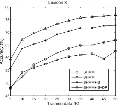
Figure 4: Accuracies of the POS tagging models using Lexicon 3

Results using Lexicon 3 are shown in Figure 4. Owing to the availability of POS-tagged sen-tences, we replace MLHMM with its supervised counterpart that is trained on the available labeled data, yielding the SHMM baseline. The accuracies of SHMM range from 48% to 67%, outperforming BHMM as the amount of labeled data increases.

5.2.2 Adding Induced Suffix Emission

Next, we augment BHMM with our first

extension, induced suffix emission, yielding BHMM+IS. For Lexicon 1, BHMM+IS achieves the same accuracy as the two baselines whend=1. The reason is simple: as all the test words are in the POS lexicon, the tagger never emits an in-duced suffix. More importantly, BHMM+IS beats BHMM and MLHMM by 4–9% and 10–14%, re-spectively. Similar trends are observed for Lex-icon 2, where BHMM+IS outperforms BHMM and MLHMM by a larger margin of 5–10% and 12–16%, respectively. For Lexicon 3, BHMM+IS outperforms SHMM, the stronger baseline, by 6– 11%. Overall, these results suggest that induced suffix emission is a strong performance-enhancing extension to G&G’s approach.

5.2.3 Adding Discriminative Prediction

Finally, we augment BHMM+IS with discrimi-native prediction, yielding BHMM+IS+DP. Since this extension requires labeled data, it can only be applied in combination with Lexicon 3. As seen in Figure 4, BHMM+IS+DP outperforms SHMM by 10–14%. Its discriminative nature proves to be

Predicted Tag Correct Tag % of Error

NN NNP 8.4

NN JJ 6.9

VM VAUX 5.9

Table 1: Most frequent POS tagging errors for BHMM+IS+DP on the 50K-word training set

strong as it even beats BHMM+IS by 3–4%.

5.2.4 Error Analysis

Table 1 lists the most common types of er-rors made by the best-performing tagging model, BHMM+IS+DP (50K-word labeled data). As we can see, common nouns and proper nouns (row 1) are difficult to distinguish, due in part to the case insensitivity of Bengali. Also, it is difficult to distinguish Bengali common nouns and adjec-tives (row 2), as they are distributionally similar to each other. The confusion between main verbs [VM] and auxiliary verbs [VAUX] (row 3) arises from the fact that certain Bengali verbs can serve as both a main verb and an auxiliary verb, depend-ing on the role the verb plays in the verb sequence.

6 Conclusions

While Goldwater and Griffiths’s fully-Bayesian approach and the traditional maximum-likelihood parameter-based approach to unsupervised POS tagging have offered promising results for English, we argued in this paper that such results were ob-tained under the unrealistic assumption that a per-fect POS lexicon is available, which renders these taggers less unsupervised than they appear. As a result, we investigated a weakly supervised fully-Bayesian approach to POS tagging, which relaxes the unrealistic assumption by automatically ac-quiring the lexicon from a small amount of POS-tagged data. Since such relaxation comes at the expense of a drop in tagging accuracy, we pro-posed two performance-enhancing extensions to the Bayesian framework, namely, induced suffix emission and discriminative prediction, which ef-fectively exploit morphology and techniques from supervised POS tagging, respectively.

Acknowledgments

References

Leonard E. Baum. 1972. An equality and associ-ated maximization technique in statistical estimation for probabilistic functions of Markov processes. In-equalities, 3:1–8.

Alexander Clark. 2000. Inducing syntactic categories by context distribution clustering. In Proceedings of CoNLL: Short Papers, pages 91–94.

Alexander Clark. 2003. Combining distributional and morphological information for part-of-speech induc-tion. In Proceedings of the EACL, pages 59–66.

Sajib Dasgupta and Vincent Ng. 2007. Unsupervised part-of-speech acquisition for resource-scarce lan-guages. In Proceedings of EMNLP-CoNLL, pages 218–227.

Arthur P. Dempster, Nan M. Laird, and Donald B. Ru-bin. 1977. Maximum likelihood from incomplete data via the EM algorithm. Journal of the Royal Sta-tistical Society. Series B (Methodological), 39:1–38.

Stuart Geman and Donald Geman. 1984. Stochas-tic relaxation, Gibbs distributions, and the Bayesian restoration of images. IEEE Transactions on Pattern Analysis and Machine Intelligence, 6:721–741.

Walter R. Gilks, Sylvia Richardson, and David J. Spiegelhalter (editors). 1996. Markov Chain Monte Carlo in Practice. Chapman & Hall, Suffolk.

Yoav Goldberg, Meni Adler, and Michael Elhadad. 2008. EM can find pretty good HMM POS-taggers (when given a good start). In Proceedings of ACL-08:HLT, pages 746–754.

John Goldsmith. 2001. Unsupervised learning of the morphology of a natural language. Computational Linguistics, 27(2):153–198.

Sharon Goldwater and Thomas L. Griffiths. 2007. A fully Bayesian approach to unsupervised part-of-speech tagging. In Proceedings of the ACL, pages 744–751.

Aria Haghighi and Dan Klein. 2006. Prototype-driven learning for sequence models. In Proceedings of HLT-NAACL, pages 320–327.

Mark Johnson. 2007. Why doesn’t EM find good HMM POS-taggers? In Proceedings of EMNLP-CoNLL, pages 296–305.

Samarth Keshava and Emily Pitler. 2006. A simpler, intuitive approach to morpheme induction. In PAS-CAL Challenge Workshop on Unsupervised Segmen-tation of Words into Morphemes.

David J. C. MacKay and Linda C. Bauman Peto. 1995. A hierarchical Dirichlet language model. Natural Language Engineering, 1:289–307.

Bernard Merialdo. 1994. Tagging English text with a probabilistic model. Computational Linguistics, 20(2):155–172.

Hinrich Sch ¨utze. 1995. Distributional part-of-speech tagging. In Proceedings of EACL, pages 141–148.

Noah A. Smith and Jason Eisner. 2005. Contrastive estimation: Training log-linear models on unlabeled data. In Proceedings of the ACL, pages 354–362.

Benjamin Snyder, Tahira Naseem, Jacob Eisenstein, and Regina Barzilay. 2008. Unsupervised multi-lingual learning for POS tagging. In Proceedings of EMNLP, pages 1041–1050.

Benjamin Snyder, Tahira Naseem, Jacob Eisenstein, and Regina Barzilay. 2009. Adding more lan-guages improves unsupervised multilingual tagging. In Proceedings of NAACL-HLT.

Yee Whye Teh, Michael Jordan, Matthew Beal, and David Blei. 2006. Hierarchical Dirichlet pro-cesses. Journal of the American Statistical Associa-tion, 101(476):1527–1554.

Kristina Toutanova and Mark Johnson. 2007. A Bayesian LDA-based model for semi-supervised part-of-speech tagging. In Proceedings of NIPS.