Modeling and Learning Semantic Co Compositionality through Prototype Projections and Neural Networks

Modeling and Learning Semantic Co-Compositionality

through Prototype Projections and Neural Networks

Masashi Tsubaki, Kevin Duh, Masashi Shimbo, Yuji Matsumoto Graduate School of Information Science

Nara Institute of Science and Technology 8916-5, Takayama, Ikoma, Nara 630-0192, Japan

{masashi-t,kevinduh,shimbo,matsu}@is.naist.jp

Abstract

We present a novel vector space model for se-mantic co-compositionality. Inspired by Gen-erative Lexicon Theory (Pustejovsky, 1995), our goal is a compositional model where both predicate and argument are allowed to modify each others’ meaning representations while generating the overall semantics. This readily addresses some major challenges with current vector space models, notably the pol-ysemy issue and the use of one represen-tation per word type. We implement co-compositionality using prototype projections

on predicates/arguments and show that this is effective in adapting their word represen-tations. We further cast the model as a neural network and propose an unsupervised algorithm to jointly train word representations with co-compositionality. The model achieves the best result to date (ρ = 0.47) on the semantic similarity task of transitive verbs (Grefenstette and Sadrzadeh, 2011).

1 Introduction

Vector space models of words have been very successful in capturing the semantic and syntactic characteristics of individual lexical items (Turney and Pantel, 2010). Much research has addressed the question of how to construct individual word representations, for example distributional models (Mitchell and Lapata, 2010) and neural models (Collobert and Weston, 2008). These word repre-sentations are used in various natural language pro-cessing (NLP) tasks such as part-of-speech tagging, chunking, named entity recognition, and semantic

V

P_company=V_kT_V k

Co-Compositionality with Prototype Projections Co-compositional vector of verb and object

start build

buy

operate =

company run

VERB run_company

Prototype Projection

company_run

OBJ

・・・ ・・・

O

firm bank

hotel

・・・ ・・・

P_run=O_kT_O k

≈

≈

× ×

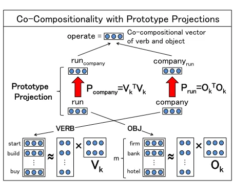
Figure 1: Here, we capture the semantics ofrunin run companyby projecting the original word representation ofrunto the prototype space ofcompany(and vice versa).

role labeling (Turian et al., 2010; Collobert et al., 2011).

Recently, modeling of semantic compositionality (Frege, 1892) in vector space has emerged as another important line of research (Mitchell and Lapata, 2008; Mitchell and Lapata, 2010; Baroni and Zam-parelli, 2010; Socher et al., 2012; Grefenstette and Sadrzadeh, 2011; Van de Cruys et al., 2013). The goal is to formulate how individual word represen-tations ought to be combined to achieve phrasal or sentential semantics.

The main questions for semantic compositionality that we are concerned with are: (1) how can poly-semy be handled by a single vector representation per word type, learned by either a distributional or neural model, and (2) how does composition resolve

these ambiguities. To this end, we are inspired by the idea of type coercion and co-compositionality

in Generative Lexicon Theory (Pustejovsky, 1995). Co-compositionality advocates that instead of a predicate-argument view of composition, both pred-icate and argument influence/coerce each other to generate the overall meaning. For example, consider a polysemous word likerun:

• (a) He runs the company.

• (b) He runs the marathon.

Run may have several senses, but the prototypical verbs that select for company differ from those that select for marathon, and thus the ambiguity at the word level is resolved at the sentence level. The same is true for the other direction, where the predicate also coerces meaning to the argument to fit expectation.

We believe that models for semantic com-position ought to incorporate elements of co-compositionality. We propose such a model here, using what we callprototype projections. For each predicate, we transform its vector representation by projecting it into a latent space that is prototypical of its argument. This projection is performed anal-ogously for each argument as well, and the final meaning is computed by composition of these trans-formed vectors (Figure 1). In addition, the model is cast as a neural network where word representations could be re-trained or fine-tuned.1

Our contributions are two-fold:

1. We propose a novel model for semantic co-compositionality. This model, based on prototype projections, is easy to implement and achieves state-of-the-art performance in the sentence similarity dataset developed by Grefenstette and Sadrzadeh (2011).

2. Our results empirically confirm that existing word representations (eg., SDS and NLM in Section 2) are sufficiently effective at capturing

1

While we are inspired by co-compositionality, it is impor-tant to note that our model does not implement qualia structure and other important components of Generative Lexicon Theory. We operate within the vector space model of distributional semantics, so these ideas are implemented with matrix algebra, which is a natural fit with neural networks.

polysemy, as long as we have the proper mech-anism to tease out the proper sense during com-position. We further propose an unsupervised neural network training algorithm that jointly fine-tunes the word representations within the co-composition model, resulting in even better performance on the sentence similarity task.

We would like to emphasize the second contribu-tion especially. Semantics research is divided in two strands, one focusing on learning word represen-tations without consideration for compositionality, and the other focusing on compositional semantics using the representations only as an input. But issues are actually related from the linguistics perspective, and even more so if we adopt a Generative Lexicon perspective. Our neural network model bridges these two strands of research by modeling co-compositionality and learning word representations simultaneously. We note that methods using context effects have been explored by Erk and Pad´o (2008; 2009) and Thater et al. (2010; 2011), but to the best of our knowledge, ours is the first model to perform co-compositionality and learning of word representations jointly.

In the following, we first provide background to the word representations employed here (Section 2). We describe the model for co-compositionality in Section 3 and the corresponding neural network in Section 4. Evaluation and experiments are presented in Sections 5 and 6. Finally, we end with related work (Section 7) and conclusions (Section 8).

2 Word Vector Representations

2.1 Simple Distributional Semantic space (SDS) word vectors

Word meaning is often represented in a high di-mensional space, where each element corresponds to some contextual element in which the word is found. Mitchell and Lapata (2010) present a co-occurrence-based semantic space called Simple Distributional Semantic space (SDS). Their SDS model uses a con-text window of five words on either side of the target word and 2,000 vector components, representing the most frequent context words (excluding a list of stop words). These components vi(t) were set to the

target word to the probability of the context word overall:

vi(t) =

p(ci|t)

p(ci)

= f reqci,t×f reqtotal

f reqt×f reqci

(1)

wheref reqci,t,f reqtotal,f reqt and f reqci are the

frequencies of the context word ci with the target

word t, the total count of all word tokens, the frequency of the target word t, and the frequency of the context wordci, respectively.

2.2 Neural Language Model (NLM) word embeddings

Another popular way to learn word representations is based on the Neural Language Model (NLM) (Bengio et al., 2003). In comparison with SDS, NLM tend to be low-dimensional (e.g. 50 dimen-sions) but employ dense features. These dense feature vectors are usually called word embeddings, and it has been shown that such vectors can cap-ture interesting linear relationships, such asking−

man+ woman ≈ queen (Mikolov et al., 2013).

In this work, we adopt the model by Collobert and Weston (2008). The idea is to construct a neural network based on word sequences, where one outputs high scores for n-grams that occur in a large unlabeled corpus and low scores fornonsense

n-grams where one word is replaced by a random word. This word representation with NLM has been used to good effect, for example in (Turian et al., 2010; Collobert et al., 2011; Huang et al., 2012) where induced word representations are used with sophisticated features to improve performance in various NLP tasks.

Specifically, we first represent the word sequence as a vectorx= [d(w1);d(w2);. . .;d(wm)], where

wi is ith word in the sequence, m is the

win-dow size, d(w) is the vector representation of word w (an n-dimensional column vector) and

[d(w1);d(w2);. . .;d(wm)]is the concatenation of

word vectors as an input of neural network. Second, we compute the score of the sequence,

score(x) =sT(tanh(Wx+b)) (2)

where W ∈ Rh×(mn) and s ∈ Rh are the first and second layer weights of the neural network, and b ∈ Rh _{is the bias unit of hidden layer. The}

superscriptT represents transposition, andtanhis applied element-wise. We also create a corrupted sequencexc = [d(w1);d(w2);. . .;d(wm′)]where

wm′ is chosen randomly from the vocabulary. We

compute the score of this implicit negative sequence

xc with the same neural network, score(xc) =

sT_(tanh(Wx

c + b)). Finally, we get the cost

function of this training algorithm as follow.

J = max(0,1−score(x) +score(xc)) (3)

In order to minimize this cost function, we optimize the parametersθ=(s,W,b,x)via backpropagation with stochastic gradient descent (SGD).

3 The Model

3.1 Prototype Projection

Generative Lexicon Theory (Pustejovsky, 1995) makes a distinction between accidental polysemy (homonyms, e.g. bank as financial institution vs. as river side) and logical polysemy (e.g. figure and ground meanings ofdoor). Our model handles both cases using the concept of projection to latent proto-typespace. The fundamental idea is that for each word w and a syntactic/semantic (binary) relation

R (such as verb-object relation), w has a set of prototype words with which it frequently occurs in relationR. For example, if w is a wordcompany, and R is the object-verb relation, prototype words should include start, build, and buy (Figure 1). For each word-relation pair, we pre-compute the latent semantic subspace spanned by these prototype words.

Later, when we encounter a phrase expressing a relationRbetween two wordsw1andw2, each word

is first projected onto a latent subspace determined by the other word and relation R. The projection operation shifts the meaning of individual words in accordance with context, and through this operation we realize coercion/co-composition. And finally, the meaning of the phrase is computed from the two projected points in the semantic space.

verb object landmark similarity(verb, landmark) similarity(projected verb, landmark)

run company operate 0.40 0.70

meet criterion satisfy 0.49 0.71

spell name write 0.04 0.50

Table 1: Examples of verb-object pairs. Original verb and landmark verb similarity, prototype projected verb and landmark verb similarity, as measure by cosine using Collobert and Weston’s word embeddings. Meethas a abstract meaning itself, but after prototype projection with matrix constructed by word vectors ofW(VerbOf,criterion),meet

is more close to meaning ofsatisfy.

company, and R = VerbOf is the object-verb

relation,

W(VerbOf,company) ={start,build, . . . ,buy}.

Now let W(R, w0) = {w1, w2,· · ·, wm} be

them prototype words we collected, and let d(w)

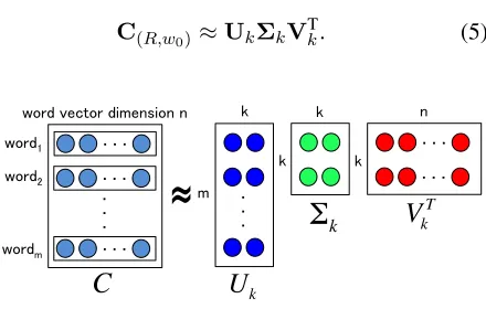
denote then-dimensional (column) vector represen-tation of wordw(either by SDS or NLM representa-tion). We make anm×nmatrixC_(R,w0)by stacking the prototype word vectors, i.e.,

C(R,w0)= [d(w1),d(w2),· · ·,d(wm)]

T ₍₄₎

and then apply Singular Value Decomposition (SVD) to extract the latent space from this matrix:

C_(R,w0)≈UkΣkVTk. (5)

word1

word vector dimension n

word2

wordm

m

・ ・ ・

・　

・　

・

k

k

n

・ ・ ・

・ ・ ・

・　

・　

・

・ ・ ・

・ ・ ・

k

k

Σ

V

U

C

≈

Figure 2: Graphical representation of SVD in our model.

Figure 2 shows the graphical representation of this matrix factorization. In NLP tasks, SVD is often applied to a term-document matrix, but in our model, we apply SVD to the matrix consisting of word vectors.

Intuitively, ΣkVT_k represents the latent

sub-space formed by prototypical words W(R, w0) = {w1, w2,· · ·, wm}. We call this matrix the

proto-type spaceof wordw0with respect to relationR.

Note that the matrix of orthogonal projection onto this prototype space is given by P(R,w0) =

(ΣkVTk)T(ΣkVTk). Hence, when we observe a

rela-tionR(w0, w), the projected representation of word

w in this context is computed by prpj_(R,w0)(w)

defined as follows:

prpj_(R,w0)(w) =P(R,w0)d(w). (6)

Table 1 shows several examples of how meanings change after prototype projection using word em-beddings of Collobert and Weston (2008).2

3.2 Co-Compositionality

In order to model co-compositionality, we apply prototype projection to both the verb and the object. In particular, suppose verb iswv and object is wo,

C(VerbOf,wo) is used to project wv and C(ObjOf,wv)

is used to project wo. The vector that represents

the overall meaning of verb-object with prototype projection is computed by:

cocomp(wv, wo) =

f(prpj_(VerbOf,w

o)(wv),prpj(ObjOf,wv)(wo)) (7)

Functionfcan be a compositional computation like simple addition or element-wise multiplication of two vectors. This is graphically shown in Figure 1.

4 Unsupervised Learning of Co-Compositionality

In this section, we propose a new neural language model that learns word representations while jointly accounting for compositional semantics. One cen-tral assumption of our work (and many other works in compositional semantics) is that a single vector

2

v o z = f(v, o) s

score = sT_z

Compositional Neural Language Model (C-NLM)

verb obj

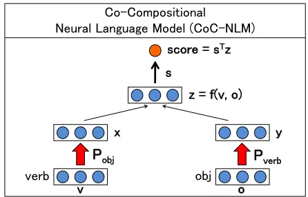
Figure 3: Compositional Neural Language Model (C-NLM).

per word type sufficiently represents the multiple meanings and usage patterns of a word.3 That means that for a polysemous word, its word vector actually represents an aggregation of the distinctly different contexts it occurs in. We will show that such an assumption is quite reasonable under our model, since the prototype projections successfully tease out the proper semantics from these aggregate representations.

However, it is natural to wonder whether one can do better if one incorporates the compositional model into the training of the word representations in the first place. To do so, we formulate a nov-el modnov-el called Compositional Neural Language

Model (Section 4.1). This model is a combination

of an unsupervised training algorithm with basic compositionality (addition/multiplications). Then, we extend this model with the projection idea in section 3.2 to formulate aCo-Compositional Neural

Language Model(Section 4.2).

4.1 Compositional Neural Language Model (C-NLM)

Compositional Neural Language Model (C-NLM)

is a combination of a word representation learning method and compositional rule. In contrast to other compositional models based on machine learning, our model has no complex parameters for model-ing composition. Composition is modeled using straightforward vector addition/multiplications; in-stead, what is learned is the word representation.

Figure 3 shows the C-NLM. The learning al-gorithm is unsupervised, and works by artificially

3_{There are works on multiple representations, e.g.,}

(Reisinger and Mooney, 2010); we focus on single represen-tation here.

z = f(v, o) s

score = sT_z

P_obj P_verb

Co-Compositional

Neural Language Model (CoC-NLM)

v o

y x

verb obj

Figure 4: Co-Compositional Neural Language Model (CoC-NLM) is C-NLM with prototype projection.

generating negative examples in a fashion analogous to the NLM learning algorithm of (Collobert and Weston, 2008) and contrastive estimation (Smith and Eisner, 2005). First, given some initial word representations and raw sentences, we compute the compositional vector with function f (in this sec-tion, we will assume that we will be using the addition operator). Second, in order to obtain the score of compositional vector, we compute the dot product with vectors ∈ Rn(nis the dimension of the word vector space): verb vectorv=d(wv)and

object vectoro=d(wo).

score(v,o) =sTf(v,o) =sT(v+o) (8)

We also create a corrupted pair by substituting a ran-dom verbwverb′. The cost functionJ = max(0,1−

score(v,o) +score(vc,o)), wherevc is the word

vector ofwverb′, encourages that the score of correct

pair is higher than the score of the corrupt pair. Let

z=v+o, our model parameters areθ= (s,z,v). The optimization is divided into two steps:

1. Optimizesandzvia SGD.

2. Letznew be the updated zvia step 1. The new

verb vector vnew trained within additive

composi-tionality is justvnew = znew −o. Note that if we

also want to optimizeo, we may want to also corrupt the object and run SGD in step 2 as well.

4.2 Co-Compositional Neural Language Model (CoC-NLM)

Language Model(CoC-NLM). We define the score function as dot product ofsand additional vector of prototype projected vectors (Figure 4). LetPobj =

P(VerbOf,wo)andPverb=P(ObjOf,wv),

score(v,o) =sT(Pobjv+Pverbo). (9)

Let x = Pobjv, y = Pverbo and z = x+ y.

Our model parameters are θ = (s,z,v). The optimization algorithm of CoC-NLM is divided into three steps like C-NLM. First, we optimize s and

z. Second, the projected verb vector is updated as xnew = znew − y. Finally we optimize v to

minimize the Euclidean distance betweenxnew and

Pobjv, whereλis a regularization hyper-parameter:

J(v) = 1

2||xnew−Pobjv||

2₊ λ

2v T_v

(10)

5 Evaluation

5.1 Dataset

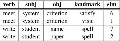
In order to evaluate the performance of our new co-compositional model with prototype projection and word representation learning algorithm, we make use of the disambiguation task of transitive sentences developed by Grefenstette and Sadrzadeh (2011). This is an extension of the two words phrase similarity task defined in Mitchell and Lapata (2008), and constructed according to similar guide-lines. The dataset consists of similarity judgments between alandmarkverb and a triple consisting of a transitive target verb, subject and object extracted from the BNC corpus. Human judges give scores between 1 to 7, with higher scores implying higher semantic similarity. For example, Table 2 shows some examples from the data: we see that the verb

meet with subject system and object criterion is judged similar to the landmark verbsatisfybut not

visit. The dataset contains a total of 2500 similarity judgements, provided by 25 participants.4 The task is to have the model produce a score for each pair of landmark verb and verb-subject-object triple. Models are evaluated by computing the Spearman’s

ρ correlation between its similarity scores and that of the human judgments.

4_{http://www.cs.ox.ac.uk/}

people/edward.grefenstette/

verb subj obj landmark sim meet system criterion satisfy 6 meet system criterion visit 1 write student name spell 7 write student paper spell 2

Table 2: Examples from the disambiguation task de-veloped by Grefenstette and Sadrzadeh (2011). Human judges give scores between 1 to 7, with higher scores implying higher semantic similarity. Verb meet with subjectsystem and object criterionis judged similar to the landmark verbsatisfybut notvisit.

5.2 Baselines

We compare our model against multiple baselines for semantic compositionality:

1. Mitchell and Lapata’s (2008) additive and element-wise multiplicative model as simplest baselines.

2. Grefenstette and Sadrzadeh’s (2011) model based on the abstract categorical framework (Coecke et al., 2010). This model computes the outer product of the subject and object vector, the outer product of the verb vector with itself, and then the element-wise product of both results.

3. Erk and Pad´o’s (2008) model, which adapts the word vectors based on context and is the most similar in terms of motivation to ours.

4. Van de Cruy et al. (2013) multi-way interaction model based on matrix factorization. This achieves the best result for this task to date.

A detailed explanation of these models will be provided in Section 7. For the underlying word rep-resentations, we experiment with sparse 2000-dim SDS and dense 50-dim NLM. These are provided by Blacoe and Lapata (2012)5 and trained on the British National Corpus (BNC). We are interested in knowing how sensitive each model is to the underlying word representation. In general, this is a challenging task: the upper-bound ofρ = 0.62is the inter-annotator agreement.

5_{http://homepages.inf.ed.ac.uk/}

5.3 Implementation details

In terms of implementation detail, our model and our re-implementation of Erk and Pado’s model make use of the ukWaC corpus (Baroni et al., 2009).6This corpus is a two billion word corpus automatically harvested from the web and parsed by the Malt-Parser (Nivre et al., 2006). We use ukWaC corpus to collect W(VerbOf, wo) and W(ObjOf, wv) for

prototype projections. We also extract about 5000 verb-object pairs that relevant for testdata from this corpus to train our neural network learning algorith-m. In our co-compositional model, the contribution ratio of SVD is set to 80% (i.e. automatically fixingk in SVD to include 80% of the top singular values). We set the number of prototype vectors to be m = 20, where W(VerbOf, wo) is filtered

with high frequency words and W(ObjOf, wv) is

filtered with both high frequency and high similarity words. In our model, we output the scores for SVO triple sentence dataset as (subject=ws, verb=wv,

object=wo,f= Addition/Multiplication):

cocomp(ws, wv, wo) =

f(d(ws),cocomp(wv, wo)) (11)

6 Results and Discussion

6.1 Main Results: The Correlation

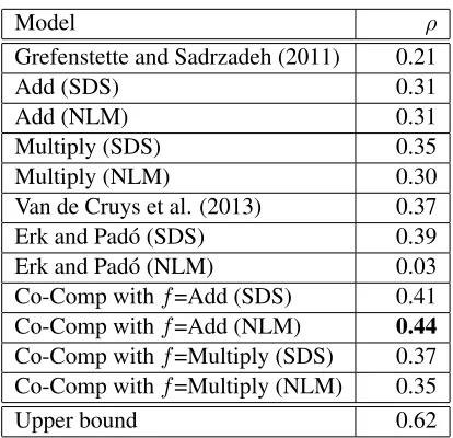
Table 3 shows the correlation scores of various models. Our observations are as follows:

1. The best reported result for this task (Van de Cruys et al., 2013) is ρ = 0.37. Our model (with NLM as word representation and

f=Addition as operator) achieves ρ = 0.44, outperforming it by a large margin. To the best of our knowledge, this is now state-of-the-art result for this task.

2. Our model is not very sensitive to the underly-ing word representation. Withf=Addition, we haveρ = 0.41for SDS vsρ = 0.44for NLM. With f=Multiply, we haveρ = 0.37for SDS vs. ρ = 0.35 for NLM. This implies that the prototype projection is robust to the underlying word representation, which is a desired charac-teristic of compositional models.

6_{http://wacky.sslmit.unibo.it/}

doku.php?id=corpora

Model ρ

Grefenstette and Sadrzadeh (2011)  0.21

Add (SDS)  0.31

Add (NLM)  0.31

Multiply (SDS)  0.35

Multiply (NLM)  0.30

Van de Cruys et al. (2013) 0.37

Erk and Pad´o (SDS) 0.39

Erk and Pad´o (NLM) 0.03

Co-Comp withf=Add (SDS) 0.41 Co-Comp withf=Add (NLM)  0.44 Co-Comp withf=Multiply (SDS) 0.37 Co-Comp withf=Multiply (NLM) 0.35

Upper bound  0.62

Table 3: Results of the different compositionality models on the similarity task. The number of prototype words

m= 20in all our models. Our model (f=Addition and NLM) achieves the new state-of-the-art performance for this task (ρ= 0.44).

3. The contextual model of Erk and Pad´o (SDS) also performed relatively well (ρ = 0.39), in fact outperforming the Van de Cruy et al. (2013) result as well. This means that the general idea of adapting word representations based on context is a very powerful one. How-ever, Erk and Pad´o’s model using the NLM rep-resentation is extremely poor (ρ = 0.03). The reason is that it uses a product operation under-the-hood to adapt the vectors, which inherently assumes a sparse representation. In this sense, our projection approach is more robust.

The state-of-the-art result for our model in Table 3 does not yet make use of the training algorithm described in Section 4. It is simply implementing the co-compositionality idea using prototype projec-tions (Section 3.2). Next in Section 6.2 we will show additional gains using unsupervised learning.

6.2 Improvements from unsupervised learning

model original representation re-trained

C-NLM 0.31 0.38

CoC-NLM 0.44  0.47

Table 4: Results of re-training the word representation for C-NLM and CoC-NLM. Learning rate α = 0.01, regularizationλ= 10−4_{and iteration = 20. One iteration} is one run through the dataset of 5000 verb-object pairs which we made from the ukWaC corpus.

NLM. Table 4 shows the gains in correlation score. This result shows that our learning model suc-cessfully captures good representation within co-compositionality of additive model. In contrast to other previous compositional models, our model does not require estimating a large number of pa-rameters for computation of compositional vectors and word representation itself is more suitable for it. Furthermore, learning is very fast, taking about 10 minutes for C-NLM on a standard machine with Intel Core i7 2.93Ghz CPU and 8GB of RAM.

6.3 The number of prototype words

The number of prototype words (min Figure 1) we use to generate the prototype space is one hyper-parameter that our model has. Here, we analyze the effect of the choice ofm. Figure 5 shows the rela-tion ofmand the performance of co-compositional model with prototype projections using either SDS or NLM representations. In general, both NLM and SDS show relatively smooth and flat curves across m, indicating the relative robustness of the approach. Nevertheless, results do degrade for large

m, due to increase in noise from non-prototype words. Further, it does appear that NLM has a slow-er drop in correlation with increasing mcompared with SDS. This suggests that NLM is more robust, which is possibly attributable to the dense and low-dimensional distributed features.

6.4 Variations in model configuration

We have presented a compositional model of the

form d(ws) + cocomp(wv, wo), where prototype

projections are performed on both wv and wo and

wsis composed as is without projection. In general,

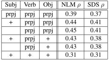
we have the freedom to choose what to project and what not to project under this co-compositional framework. Here in Table 5 we show the results of

Figure 5: The relation between the number of prototype words and correlation of SDS or NLM. In general, NLM has higher correlation than SDS and is more robust across them.

Subj Verb Obj NLMρ SDSρ

prpj prpj prpj 0.39 0.37 + prpj prpj 0.44 0.41 prpj prpj 0.45 0.41

+ prpj + 0.43 0.38

prpj + 0.43 0.38

+ + + 0.31 0.31

Table 5: Variants of the full co-compositional model, based on how subject, verb, and object vector repre-sentations are included. prpj indicates that prototype projection is used. + indicates that the vector is added without projection first. Blank indicates that the vector is not used in the final compositional score.

these variants, using f =Addition and SDS/NLM representations without re-training. We note that our positive results mainly come from the verb projections. Subject information actually does not help. We believe this best configuration is task-dependent; in this test collection, the subjects appear to have little contribution to the landmark verb.

7 Related work

One of the first approaches is the vector ad-dition/multiplication idea of Mitchell and Lapata (2008). The appeal of this kind of simple approach is its intuitive geometric interpretation and its ro-bustness to various datasets. However, it may not be sufficiently expressive to represent the various factors involved in compositional semantics, such as syntax and context. To this end, Baroni and Zamparelli (2010) present a compositional model for adjectives and nouns. In their model, an adjective is a matrix operator that modifies the noun vector into an adjective-noun vector. Zanzotto et al. (2010) and Guevara (2010) also proposed linear transfor-mation models for composition and address the issue of estimating large matrices with least squares or regression techniques. Socher et al. (2012) extend this linear transformation approach with the more powerful model of Matrix-Vector Recursive Neural Networks (MV-RNN). Each node in a parse tree is assigned both a vector and a matrix. The vector captures the actual meaning of the word itself, while the matrix is modeled as a operator that modify the meaning of neighboring words and phrases. This model captures semantic change phenomenon like

not bad is similar to good due to a composition

of thebad vector with a meaning-flippingnot ma-trix. But this MV-RNN also need to optimize all matrices of words from initial value (identity plus a small amount of Gaussian noise) with supervised dataset like movie reviews. Our prototype projection model is similar to these models as a matrix-vector operation, except that the matrix is not learned and computed from prototype words. In future work, we can imagine integrating the two models, using these prototype projection matrices as initial values for MV-RNN training (Socher et al., 2012).

Another approach is exemplified by Coecke et al. (2010). In their mathematical framework u-nifying categorical logic and vector space models, the sentence vector is modeled as a function of the Kronecker product of its word vectors. Grefenstette and Sadrzadeh (2011) implement this based on un-supervised learning of matrices for relational words and apply them to the vectors of their arguments. Their idea is that words with relational types, such as verbs, adjectives, and adverbs are matrices that act as a filter on their arguments. They also developed a new semantic similarity task based on transitive

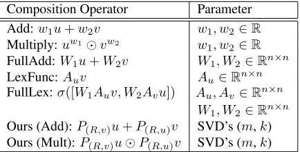
Composition Operator Parameter Add:w1u+w2v w1, w2∈R Multiply:uw1⊙_vw2 _w

1, w2∈R FullAdd:W1u+W2v W1, W2∈Rn×n LexFunc:Auv Au∈Rn×n

FullLex:σ([W1Auv, W2Avu])

Au, Av∈Rn×n

W1, W2∈Rn×n Ours (Add):P(R,v)u+P(R,u)v SVD’s (m,k) Ours (Mult):P(R,v)u⊙P(R,u)v SVD’s (m,k)

Table 6: Comparison of composition operators that com-bine two word vector representations, u, v ∈ Rn _and

their learning parameters. Our model only needs two hyper-parameters: the number of prototype wordsmand dimensional reductionkin SVD

verbs, which is the dataset we used here. The pre-vious state-of-the-art result for this task comes from the model of Van de Cruys et al. (2013). They model compositionality as a multi-way interaction between latent factors, which are automatically constructed from corpus data via matrix factorization.

Comprehensive evaluation of various existing models are reported in (Blacoe and Lapata, 2012; D-inu et al., 2013). Blacoe and Lapata (2012) highlight the importance of jointly examining word represen-tations and compositionality operators. However, two out of three composition methods they evaluate are parameter-free, so that they can side-step the issue of parameter estimation. Dinu et al. (2013) de-scribe the relation between word vector and compo-sitionality in more detail with free parameters. Table 6 summarizes some ways to compose the meaning of two word vectors (u, v), following (Dinu et al., 2013). These range from simple operators (e.g. Add and Multiply) to expressive models with many free parameters (e.g. LexFunc, FullLex). Many of these models need to optimizen×n parameters, which may be large. On the other hand, our model only needs two hyper-parameters: the number of proto-type wordsmand dimensional reductionk in SVD (Table 6). Furthermore, our model performance with neural language model word embeddings is robust to variations inm.

prefer-ence information for subjects, verbs, and objects in context; our prototype word vectors are essentially equivalent to this idea. The main difference is in how we modify the target word representation v

using this information: whereas we projectv onto a latent subspace formed by collection of prototype vectors, Erk and Pad´o (2008; 2009) and Thater et al. (2010; 2011) use the prototype vectors to directly modify the elements ofv, i.e. by element-wise product with the centroid prototype vector. Intuitively, both our method and theirs essentially delete part of a word vector representation to adapt the meaning in context. We believe the projection is more robust to the underlying word representation (and this is shown in the results for SDS vs. NLM representations), but we note that we may be able to borrow some of more sophisticated ways to find prototype vectors from Erk and Pad´o (2008; 2009) and Thater et al. (2010; 2011).

8 Conclusion and Future Work

We began this work by asking how it is possible to handle polysemy issues in compositional semantics, especially when adopting distributional semantics methods that construct only one representation per word type. After all, the different senses of the same word are all conflated into a single vector representation. We found our inspiration in Gen-erative Lexicon Theory (Pustejovsky, 1995), where ambiguity is resolved due toco-compositionalityof the words in the sentence, i.e., the meaning of an ambiguous verb is generated by the properties the object it takes, and vice versa. We implement this idea in a novel neural network model using proto-type projections. The advantages of this model is that it is robust to the underlying word representation used and that it enables an effective joint learning of word representations. The model achieves the current state-of-the-art performance (ρ = 0.47) on the semantic similarity task of transitive verbs (Grefenstette and Sadrzadeh, 2011).

Directions for future research include:

• Experiments on other semantics tasks, such as paraphrase detection, word sense induction, and word meaning in context.

• Extension to more holistic sentence-level

com-position using a matrix-vector recursive frame-work like (Socher et al., 2012).

• Explore further the potential synergy between Distributional Semantics and the Generative Lexicon.

Acknowledgments

This work was partially supported by JSPS KAK-ENHI Grant Number 24800041, JSPS KAKKAK-ENHI 2430057 and Microsoft Research CORE Project. We would like to thank Hiroyuki Shindo and anony-mous reviewers for their helpful comments.

References

Marco Baroni and Roberto Zamparelli. 2010. Nouns are vectors, adjectives are matrices: Representing adjective-noun constructions in semantic space. In

Proceedings of the Conference on Empirical Methods in Natural Language Processing (EMNLP).

Marco Baroni, Silvia Bernardini, Adriano Ferraresi, and Eros Zanchetta. 2009. The wacky wide web: A collection of very large linguistically processed web-crawled corpora. Language resources and evaluation, 43(3):209–226.

Marco Baroni, Raffaella Bernardi, and Roberto Zampar-elli. 2013. Frege in space: A program for compo-sitional distributional semantics. Linguistic Issues in Language Technologies.

Yoshua Bengio, R´ejean Ducharme, Pascal Vincent, and Christian Janvin. 2003. A neural probabilistic lan-guage model.Journal of Machine Learning Research, 3:1137–1155.

William Blacoe and Mirella Lapata. 2012. A comparison of vector-based representations for semantic composi-tion. InProceedings of the Joint Conference on Em-pirical Methods in Natural Language Processing and Computational Natural Language Learning (EMNLP-CoNLL).

Bob Coecke, Mehrnoosh Sadrzadeh, and Stephen Clark. 2010. Mathematical foundations for a composi-tional distribucomposi-tional model of meaning. CoRR, ab-s/1003.4394.

Ronan Collobert and Jason Weston. 2008. A unified architecture for natural language processing: Deep neural networks with multitask learning. In Pro-ceedings of the International Conference on Machine Learning (ICML).

Journal of Machine Learning Research, 12:2493– 2537.

Georgiana Dinu, Nghia The Pham, and Marco Barori. 2013. General estimation and evaluation of composi-tional distribucomposi-tional semantic models. InProceedings of the Workshop on Continuous Vector Space Models and their Compositionality.

Katrin Erk and Sebastian Pad´o. 2008. A structured vector space model for word meaning in context. In

Proceedings of the Conference on Empirical Methods in Natural Language Processing (EMNLP).

Katrin Erk and Sebastian Pad´o. 2009. Paraphrase assess-ment in structured vector space: Exploring parameters and datasets. In Proceedings of the Workshop on Geometrical Models of Natural Language Semantics. Katrin Erk. 2012. Vector space models of word meaning

and phrase meaning: A survey. Language and Lin-guistics Compass, 6(10):635–653.

G Frege. 1892. ¨Uber sinn und bedeutung. InZeitschfrift f¨ur Philosophie und philosophische Kritik, 100. Edward Grefenstette and Mehrnoosh Sadrzadeh. 2011.

Experimental support for a categorical compositional distributional model of meaning. In Proceedings of the Conference on Empirical Methods in Natural Language Processing (EMNLP).

Emiliano Guevara. 2010. A regression model of adjective-noun compositionality in distributional se-mantics. InProceedings of the Workshop on GEomet-rical Models of Natural Language Semantics. Eric Huang, Richard Socher, Christopher Manning, and

Andrew Ng. 2012. Improving word representations via global context and multiple word prototypes. In

Proceedings of the Annual Meeting of the Association for Computational Linguistics (ACL).

Tomas Mikolov, Wen-tau Yih, and Geoffrey Zweig. 2013. Linguistic regularities in continuous space word representations. In Human Language Technologies: The Conference of the North American Chapter of the Association for Computational Linguistics (NAACL-HLT).

Jeff Mitchell and Mirella Lapata. 2008. Vector-based models of semantic composition. In Proceedings of the Annual Meeting of the Association for Computa-tional Linguistics (ACL).

Jeff Mitchell and Mirella Lapata. 2010. Composition in distributional models of semantics.Cognitive Science, 34(8):1388–1439.

Joakim Nivre, Johan Hall, and Jens Nilsson. 2006. Maltparser: A data-driven parser-generator for depen-dency parsing. In Proceedings of the International Conference on Language Resources and Evaluation (LREC).

James Pustejovsky. 1995. The Generative Lexicon. MIT Press, Cambridge, MA.

Joseph Reisinger and Raymond J Mooney. 2010. Multi-prototype vector-space models of word meaning. In

Human Language Technologies: The Conference of the North American Chapter of the Association for Computational Linguistics (NAACL-HLT).

Noah A. Smith and Jason Eisner. 2005. Contrastive estimation: Training log-linear models on unlabeled data. In Proceedings of the Annual Meeting of the Association for Computational Linguistics (ACL). Richard Socher, Brody Huval, Christopher D. Manning,

and Andrew Y. Ng. 2012. Semantic compositionality through recursive matrix-vector spaces. In Proceed-ings of the Joint Conference on Empirical Methods in Natural Language Processing and Computational Natural Language Learning (EMNLP-CoNLL). Stefan Thater, Hagen F¨urstenau, and Manfred Pinkal.

2010. Contextualizing semantic representations using syntactically enriched vector models. InProceedings of the Annual Meeting of the Association for Compu-tational Linguistics (ACL).

Stefan Thater, Hagen F¨urstenau, and Manfred Pinkal. 2011. Word meaning in context: A simple and effective vector model. InAsian Federation of Natural Language Processing (IJCNLP).

Joseph Turian, Lev-Arie Ratinov, and Yoshua Bengio. 2010. Word representations: A simple and general method for semi-supervised learning. InProceedings of the Annual Meeting of the Association for Compu-tational Linguistics (ACL).

Peter D Turney and Patrick Pantel. 2010. From fre-quency to meaning: Vector space models of semantics.

Journal of artificial intelligence research, 37(1):141– 188.

Tim Van de Cruys, Thierry Poibeau, and Anna Korhonen. 2013. A tensor-based factorization model of semantic compositionality. InHuman Language Technologies: The Conference of the North American Chapter of the Association for Computational Linguistics (NAACL-HLT).