Contextual Bidirectional Long Short Term Memory Recurrent Neural Network Language Models: A Generative Approach to Sentiment Analysis

Contextual Bidirectional Long Short-Term Memory Recurrent Neural

Network Language Models:

A Generative Approach to Sentiment Analysis

1_{Chair of Complex & Intelligent Systems, University of Passau, Passau, Germany} 2_{Department of Computing, Imperial College London, London, UK}

amr.mousa@uni-passau.de schuller@ieee.org

Abstract

Traditional learning-based approaches to sentiment analysis of written text use the concept of bag-of-words or bag-of-n -grams, where a document is viewed as a set of terms or short combinations of terms disregarding grammar rules or word order. Novel approaches de-emphasize this concept and view the problem as a sequence classification problem. In this context, recurrent neural networks (RNNs) have achieved significant success. The idea is to use RNNs as discriminative bi-nary classifiers to predict a positive or neg-ative sentiment label at every word posi-tion then perform a type of pooling to get a sentence-level polarity. Here, we investi-gate a novel generative approach in which a separate probability distribution is esti-mated for every sentiment using language models (LMs) based on long short-term memory (LSTM) RNNs. We introduce a novel type of LM using a modified version of bidirectional LSTM (BLSTM) called contextual BLSTM (cBLSTM), where the probability of a word is estimated based on its full left and right contexts. Our ap-proach is compared with a BLSTM binary classifier. Significant improvements are observed in classifying the IMDB movie review dataset. Further improvements are achieved via model combination.

1 Introduction

Sentiment analysis of text (also known as opinion mining) is the process of computationally identify-ing and categorizidentify-ing opinions expressed in a piece of text in order to determine the writer’s attitude towards a particular topic. Due to the tremendous

increase in web content, many organizations be-came increasingly interested in analyzing this big data in order to monitor the public opinion and as-sist decision making. Therefore, sentiment analy-sis attracted the interest of many researchers.

The task of sentiment analysis can be seen as a text classification problem. Depending on the tar-get of the analysis, the classes can be described by continuous primitives such as valence, a polarity state (positive or negative attitude), or a subjectiv-ity state (objective or subjective). In this work, we are interested in the binary classification of doc-uments into a positive or negative attitude. Such detection of polarity is a non-trivial problem due to the existence of noise, comparisons, vocabulary changes, and the use of idioms, irony, and domain specific terminology (Schuller et al., 2015).

Traditional approaches to sentiment analysis rely on the concept of bag-of-words or bag-of-n -grams, where a document is viewed as a set of terms or short combinations of terms disregarding grammar rules or word order. In this case, usually, the analysis involves: tokenization and parsing of text documents, careful selection of important fea-tures (terms), dimensionality reduction, and clas-sification of the documents into categories. For ex-ample, Pang et al. (2002) have considered different classifiers, such as Naive Bayes (NB), maximum entropy (MaxEnt), and support vector machines (SVM) to detect the polarity of movie reviews. Pang and Lee (2004) have combined polarity and subjectivity analysis and proposed a technique to filter out objective sentences of movie reviews based on finding minimum cuts in graphs. In (Taboada et al., 2011; Ding et al., 2008), lexicon-based techniques are examined, where word-level sentimental orientation scores are used to evaluate the polarity of product reviews. More advanced approaches utilize word orn-gram vectors, like in (Maas et al., 2011; Dahl et al., 2012).

Novel approaches are mainly based on artifi-cial neural networks (ANNs). These approaches de-emphasize the concept of of-words or bag-of-n-grams. A document is viewed as a set of sentences, each sentence is a sequence of words. The sentiment problem is rather considered as a sequence classification problem. For example, in (Dong et al., 2014; Dong et al., 2016), RNN clas-sifiers are used with an adaptive method to select relevant semantic composition functions for ob-taining vector representations of sentences. This is found to improve sentiment classification on the Stanford Sentiment Treebank (SST). Rong et al. (2014) have used a RNN model to learn word rep-resentation simultaneously with the sentiment dis-tribution. Santos and Gatti (2014) have proposed a convolutional neural network (CNN) that exploits from character- to sentence-level information to perform sentiment analysis on the Stanford Twit-ter Sentiment (STS) corpus. Kalchbrenner et al. (2014) have used a dynamic convolutional neu-ral network (DCNN) with a dynamick-max pool-ing to perform sentiment analysis on the SST and Twitter sentiment datasets. Lai et al. (2015) have utilized a combination of RNNs and CNNs called recurrent convolutional neural network (RCNN) to perform text classification on multiple datasets in-cluding sentiment analysis on the SST dataset.

Other novel approaches use tree structured neu-ral models instead of sequential models (like RNNs) in order to capture complex semantic re-lationships that relate words to phrases. Despite their good performance, these models rely on existing parse trees of the underlying sentences which are, in most cases, not readily available or not trivial to generate. For example, Socher et al. (2013) have introduced a recursive neural ten-sor network (RNTN) to predict the compositional semantic effects in the SST dataset. In (Tai et al., 2015; Le and Zuidema, 2015), tree-structured LSTMs are used to improve the earlier models.

Another perspective to the sentiment problem is to assume that each sentence with a positive or negative class is drawn from a particular proba-bility distribution related to that class. Then, in-stead of estimating a discriminative model that learns how to separate sentiment classes in sen-tence space, we estimate a generative model that tells us how these sentences are generated. This generative approach can be better or complemen-tary in some sense to the discriminative approach.

The probability distributions over word se-quences are well known as language models (LMs). They have also been used for sentiment analysis. However, no trial is made to go beyond simple bigram models. For example, Hu et al. (2007b) have estimated two separate positive and negative LMs from training collections. Tests are performed by computing the Kullback-Leibler di-vergence between the LM estimated from the test document and the sentiment LMs. Therein, uni-and bigram models are shown to outperform SVM models in classifying a movie review dataset. In (Hu et al., 2007a), a batch of terms in a domain are identified. Then, two different unigram LMs representing classifying knowledge for every term are built up from subjective sentences. A classi-fying function based on the generation of a test document is defined for the sentiment classifica-tion. This approach has outperformed SVM on a Chinese digital product review dataset. Liu et al. (2012) have employed an emoticon smoothed un-igram LM to perform sentiment classification.

In this paper, we compare the generative LM approach with the discriminative binary classifi-cation approach. We estimate a separate proba-bility distribution for each sentiment using long-span LMs based on unidirectional LSTMs (Sun-dermeyer et al., 2012) trained to predict a word depending on its full left context. The probability scores from positive and negative LMs are used to classify unseen sentences. In addition, we intro-duce a novel type of LM using a modified version of the standard bidirectional LSTM called contex-tual bidirectional LSTM (cBLSTM). In contrast to the unidirectional model, this model is trained to predict a word depending on its full left and right contexts. Moreover, we combine the LM approach with the binary classification approach using lin-ear interpolation of probabilities. We observe that the cBLSTM LM outperforms both the LSTM LM and the BLSTM binary classifier. Combining approaches together yields further improvements. Models are evaluated on the IMDB large movie review dataset1_{(Maas et al., 2011).}

2 Language Models

A statistical LM is a probability distribution over word sequences that assigns a probabilityp(wM

1 )

to any word sequencewM

1 of lengthM. Thus, it

provides a way to estimate the relative likelihood

of different phrases. It is a widely used model in many natural language processing tasks, like au-tomatic speech recognition, machine translation, and information retrieval. Usually, to estimate a LM, the assumption of the(n−1)th_{order Markov}

process is used (Bahl et al., 1983), in which a cur-rent wordwmis assumed conditionally dependent

on the preceding(n−1)history words, such that:

p(wM₁ )≈ YM

m=1

p(wm|wmm−−n1+1). (1)

This is called ann-gram LM. A conventional ap-proach to estimate these probabilities is the back-off LM which is based on count statistics col-lected from the training text. In addition to the initial n-gram approximation, a major drawback of this model is that it backs-off to a shorter his-tory whenever insufficient statistics are observed for a givenn-gram. Novel state-of-the-art LMs are based on ANNs like RNNs that provide long-span probabilities conditioned on all predecessor words (Mikolov et al., 2010; Kombrink et al., 2011).

3 Unidirectional RNN Models

3.1 Standard RNN

A RNN maps from a sequence of input observa-tions to a sequence of output labels. The mapping is defined by a set of activation weights and a non-linear activation function. Recurrent connections allow to access activations from past time steps. For an input sequence xT

1, a RNN computes the

hidden sequence hT

1 and the output sequence yT1

by performing the following operations for time stepst= 1toT (Graves et al., 2013):

ht = H(Wxhxt+Whhht−1+bh) (2)

yt = Whyht+by, (3)

where H is the hidden layer activation function, Wxh is the weight matrix between the input and

hidden layer, Whh is the recurrent weight

ma-trix between the hidden layer and itself, Why is

the weight matrix between the hidden and output layer, bh and by are the hidden and output layer

bias vectors respectively.His usually an element-wise application of the sigmoid function.

3.2 LSTM RNN

In (Hochreiter and Schmidhuber, 1997), an al-ternative RNN called Long Short-Term Memory (LSTM) is introduced where the conventional neu-ron is replaced with a so-calledmemory cell con-trolled by input, output and forget gates in order to

overcome the vanishing gradient problem of tradi-tional RNNs. In this case,Hcan be described by the following composite function:

it=σ(Wxixt+Whiht−1+Wcict−1+bi) (4)

ft=σ(Wxfxt+Whfht−1+Wcfct−1+bf)(5)

ct=ftct−1+ittanh(Wxcxt+Whcht−1+bc)(6)

ot=σ(Wxoxt+Whoht−1+Wcoct+bo) (7)

ht=ottanh(ct), (8)

whereσ is the sigmoid function, i,f,o, and care respectively the input, forget, output gates, and cell activation vectors (Graves et al., 2013).

3.3 LSTM LM

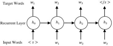
In a LSTM LM, the time steps correspond to the word positions in a training sentence. At every time step, the network takes as input the word at the current position encoded as a 1-hot binary vec-tor. The input vector is then passed to one or more recurrent hidden layers with self connections that implicitly take into account all the previous his-tory words presented to the network. The output of the final hidden layer is passed to an output layer with a softmax activation function to produce a correctly normalized probability distribution. The target output at each word position is the next word in the sentence. A cross-entropy loss function is used which is equivalent to maximizing the likeli-hood of the training data. At the end, the network can predict the long-span conditional probability p(wm|w₁m−1)for any wordwm ∈ V and a given

historywm₁ −1, whereV is the vocabulary. Fig. 1 shows an unfolded example of a LSTM LM over a sentence<s> w1 w2w3 </s>, where<s>and

</s>are the sentence start and end symbols.

</𝑠 > 𝑤2 𝑤3

𝑤3 ℎ1 ℎ2 ℎ3

𝑤1 𝑤2

Target Words

Recurrent Layer

Input Words

𝑤1

ℎ0

< 𝑠 >

Figure 1: Architecture of a LSTM LM predicting a word given its full previous history.

4 Bidirectional RNN Models

4.1 BLSTM RNN

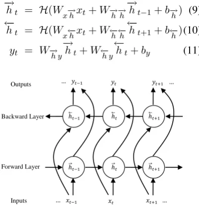
compute forward and backward hidden sequences

− →

h, ←−h respectively, which are then combined to compute the output sequencey(see Fig. 2), thus:

−

→_h

t = H(W_x−→_hxt+W−→_h−→_h−→ht−1+b−→_h) (9)

←−

ht = H(W_x←−_hxt+W←_h−←−_h←−ht+1+b←−_h)(10)

yt = W−→_{h y}−→ht+W←−_{h y}←−ht+by (11)

𝑦𝑡+1 … … 𝑦𝑡−1 𝑦𝑡

𝑥𝑡+1 … ℎ 𝑡−1

ℎ 𝑡−1

ℎ 𝑡 ℎ 𝑡

ℎ 𝑡+1 ℎ 𝑡+1

… 𝑥𝑡−1 𝑥𝑡

Outputs

Backward Layer

Forward Layer

Inputs

Figure 2: Architecture of a BLSTM, every output depends on the whole input sequence.

4.2 Contextual BLSTM LM

The standard BLSTM described in Section 4.1 is not suitable for estimating LMs. This is because it predicts every output symbol depending on the whole input sequence. Since a LM indeed uses the same word sequence in both input and target sides of the network, it would be incorrect to predict a word given the whole input sentence. Rather, it is required to predict a word given the full left and right context while excluding the predicted word itself from the conditional dependence. To allow for this, we modify the architecture of the standard BLSTM such that it accounts for a contextual de-pendence rather than a full sequence dede-pendence. The new model is called a contextual BLSTM or cBLSTM in short. The architecture of this model is illustrated in Fig. 3.

𝑤2

ℎ 0

ℎ 0

ℎ 1

ℎ 1

ℎ 2

ℎ 2

< 𝑠 > 𝑤1

Target Words

Backward Layer

Forward Layer

Inputs Words

𝑤2

< 𝑠 >

𝑤1

𝑤3

ℎ 3

ℎ 3

𝑤3

</𝑠 > </𝑠 >

Figure 3: Architecture of a cBLSTM LM predict-ing a word given its full left and right contexts.

The model consists of a forward and a backward sub-layer. The forward sub-layer receives the en-coded input words staring from the sentence start symbol up to the last word before the sentence end symbol (sequence < s > w1w2 w3 in Fig.

3). The forward hidden states are used to predict words starting from the first word after the sen-tence start symbol up to the sensen-tence end symbol (sequencew1w2w3 </s>in Fig. 3). The

back-ward sub-layer does exactly the reverse operation. The two sub-layers are interleaved together in or-der to adjust the conditional dependence such that the prediction of any target word depends on the full left and right contexts. Note that the hidden state at the first as well as the last time step needs to be padded by zeros so that the size of the hid-den vector is consistent across all time steps. At the end, the model can effectively predict the con-ditional probability p(wm|w1m−1, wmM+1) for any

wordwm ∈ V, left contextwm1 −1 and right

con-text wM

m+1, whereV is the vocabulary and M is

the length of the sentence. Table 1 shows the pre-dicted probability at each time step of Fig. 3. Note that one direction dependence is maintained at the start and end of sentence (time steps 1 and 5).

time step predicted conditional prob.

1 p(<s> |w1w2w3 </s>)

2 p(w1 |<s> , w2 w3 </s>)

3 p(w2 |<s> w1 , w3 </s>)

4 p(w3 |<s> w1 w2 , </s>)

5 p(</s> |<s> w1w2 w3)

Table 1: Predicted conditional probabilities at ev-ery time step of the cBLSTM shown in Fig. 3.

Our implementation of the novel cBLSTM RNN model is integrated into our publicly avail-able CURRENNT2 _{toolkit initially introduced by} Weninger et al. (2014). A new version of the toolkit with the novel implementations is planned to be available by the date of publication.

Here, it is worth noting that deep cBLSTM models can not be easily constructed by stacking multiple hidden bidirectional layers together. The reason is that the hidden states obtained after the first bidirectional layer are dependent on the full left and right contexts. If these states are utilized as inputs to a second bidirectional layer that identi-cally repeats the same operation again, then the de-sired conditional dependence will not be correctly

maintained. One method to solve this problem is to create deeper models by stacking multiple for-ward and backfor-ward sub-layers independently. The fusion of both sub-layers takes place and the end of the deep stack. The implementation of such a deep cBLSTM model is not yet available.

5 Dataset

Our experiments on sentiment analysis are per-formed on the IMDB large movie review dataset (v1.0) introduced by Maas et al. (2011). The la-beled partition of the dataset consists of 50k bal-anced full-length movie reviews with 25k positive and 25k negative reviews extracted from the Inter-net Movie Database (IMDB)3_.

Since the reviews are in a form of long para-graphs which are difficult to handle directly with RNNs, we break down these paragraphs into rela-tively short sentences based on punctuation clues. After breaking down the paragraphs, the average number of sentences per review is around 13 sen-tences. We randomly selected 1000 positive and 1000 negative reviews as our test set. A similar number of random reviews are selected as a devel-opment set. The remaining reviews are used as a training set. Note that this is not the official dataset division provided by Maas et al. (2011), where 25k balanced reviews are dedicated for training and the other 25k balanced reviews are dedicated for test-ing. The reasons not to follow the official divi-sion are firstly that, it does not provide a devel-opment set; secondly, our proposed models need much data to train well as revealed by initial exper-iments; thirdly, it would be very time consuming to use the whole data as one partition and perform multi-fold cross validation as usually adopted with large sentiment datasets (Schuller et al., 2015). A preprocessed version of the IMDB dataset with the modified partitioning is planned to be available for download by the date of publication.

A word list of the 10k most frequent words is se-lected as our vocabulary. This covers around 95% of the words in our development and test sets. Any out-of-vocabulary word is mapped to a specialunk

symbol. We use the classification accuracy as our evaluation measure. The unweighted average F1 scores over positive and negative classes are also calculated. However, their values are found almost similar to the classification accuracies. Therefore, only classification accuracies are reported.

3_{http://www.imdb.com}

6 Related Work

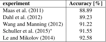
The work of this paper is closely related to several previous publications that report sentiment classi-fication accuracy on the same dataset. For exam-ple, in (Maas et al., 2011), the IMDB dataset is introduced and a semi-supervised word vector in-duction framework is used, where an unsupervised probabilistic model similar to latent Dirichlet allo-cation (LDA) is proposed to learn word vectors. Another supervised model is utilized to constrain words expressing similar sentiment to have sim-ilar representations in vector space. In (Dahl et al., 2012), documents are treated as bags of n -grams. Restricted Boltzmann machines (RBMs) are used to extract vector representations for n -grams. Then, a linear SVM model is utilized to classify documents based on the resulting feature vectors. Wang and Manning (2012) have used a variant of SVM with Naive Bayes log-count ratios as well as word bigrams as features. This modi-fied SVM model is referred to as NBSVM. In our previous publication (Schuller et al., 2015), LSTM LMs trained on 40% of the whole IMDB dataset are used for performing sentiment analysis. How-ever, a carefully tuned MaxEnt classifier is found to perform better. Le and Mikolov (2014) have used a paragraph vector methodology with an un-supervised algorithm based on feed-forward neu-ral networks that learns fixed-length vector rep-resentations from variable-length texts. All these publications use the official IMDB dataset division except for (Schuller et al., 2015), where a similar division as in this paper is used. To give a compre-hensive idea about the aforementioned techniques, we show in Table 2 the classification results as re-ported in the related publications. Note that only the results of (Schuller et al., 2015) are directly comparable to our results.

experiment Accuracy [%]

Maas et al. (2011) 88.89 Dahl et al. (2012) 89.23 Wang and Manning (2012) 91.22 Schuller et al. (2015)∗ _91.55 Le and Mikolov (2014) 92.58 Table 2: Sentiment classification accuracies from previous publications on the IMDB dataset.

LMs. For example, in (Frinken et al., 2012), dis-tinct forward and backward LMs are estimated for handwriting recognition. However, no trial is made to go beyond 4-gram models. In (Xiong et al., 2016), standard forward and backward RNN LMs are separately estimated for a conversational speech recognition task. The log probabilities from both models are added. In (Arisoy et al., 2015), bidirectional RNNs and LSTMs are used to estimate LMs for an English speech recogni-tion task. Therein, the standard bidirecrecogni-tional ar-chitecture (as in Fig. 2) is used without modifica-tions. This causes circular dependencies to arise when combining probabilities from multiple time steps. Therefore, pseudo-likelihoods are utilized rather than true likelihoods which is not perfect from the mathematical point of view. Not sur-prisingly, the BLSTM LMs do not yield any gain over the LSTM LMs. In addition, the perplexity of such a model becomes invalid. More impor-tantly, in (Peris and Casacuberta, 2015), bidirec-tional RNN LMs are used for a statistical machine translation task. However, only standard RNNs but not LSTMs are utilized. Furthermore, no de-tails are provided about how the model is exactly modified and how the left and right dependencies are maintained over time steps.

7 Sentiment Classification

7.1 Generative LM-based classifier

Our first approach to sentiment classification is the generative approach based on LMs. We either use LSTM LMs described in Section 3.3 or cBLSTM LMs described Section 4.2. Two separate LMs are estimated from positive and negative training data. We use networks with a single hidden layer that consists of 300 memory cells followed by a softmax layer with a dimension of10k+ 3. This is equal to the full vocabulary size in addition to

<s>, </s>, and unk symbols representing

sen-tence start, sensen-tence end, and unknown word sym-bols respectively. In case of using cBLSTM net-works, a single hidden layer of 600 memory cells is used (300 cells for each forward and backward sub-layer). A cross-entropy loss function is used with a momentum of 0.9. We use sentence-level mini-batches of size 100 sentences computed in parallel. The learning rate is set initially to10−3

and then decreased gradually to10−6_{. The}

train-ing process is controlled by monitortrain-ing the cross-entropy error over the development set.

In addition, we use a data sub-sampling methodology during training. For this purpose, a traditional 5-gram backoff LM is created out of the development data, we call this aranking LM. Then, all training sentences are ranked according to their perplexities with the ranking LM. Using these ranks, we divide our training sentences into three partitions that reflect the relative importance of the data, such that the first partition contains the 100k sentences with the lowest perplexities, the second partition contains the 100k sentences with next lowest perplexities. The third partition contains all the other sentences. Instead of using the whole training data in each epoch, we use a random sample with more sentences from the first two partitions than the third one. After a suffi-cient number of epochs, the whole training data is covered. The sub-sampling approach speeds up the training and makes it feasible with any size of training data. At the same time, the training is fo-cused on the relatively more important examples. In addition, it adds a useful regularization to the training process. Yet, it leads to a less smoother convergence. To show the efficiency of our sen-tence ranking methodology, Table 3 shows exam-ples of the highest and lowest ranked sentences from positive and negative training data.

most +ve this is one of the best films

ever made.

least +ve cheap laughs but great value.

most -ve this is one of the worst movies

i have ever seen.

least -ve life’s too short.

Table 3: Examples of the highest/lowest ranked sentences from positive/negative training data.

After training the neural networks, each of the positive and negative sentiment LM estimates a probability distribution for the corresponding sen-timent, we call these probability distributionsp+

and p−. To evaluate the sentiment of some test review, we calculate the perplexity of each model p+andp−with respect to the whole review. Thus, given a probability distributionp, and a review text Scomposed ofK sentencesS =s1, ..., sK, each

sentence sk : 1 ≤ k ≤ K is composed of a

se-quence of Mk words sk = w1k, w2k, ..., wMkk; we

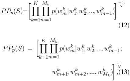
calculate the perplexityP Pp(S)of a modelpwith

measure-ment of how well a probability distribution pre-dicts a sample. A low perplexity indicates that the probability distribution is good at predicting the sample. Perplexity is defined as the exponentiated negative average log-likelihood, or in other words, the inverse of the geometric average probability assigned by the model to each word in the sam-ple. We calculate the Perplexity using Equation 12 if the model p is based on LSTM, and using Equation 13 if the model is based on cBLSTM:

P Pp(S)=

_YK

k=1 Mk Y

m=1

p(wk_m|w₁k, wk₂, ..., w_mk₋₁)

−1

N

(12)

P Pp(S) =

_YK

k=1 Mk Y

m=1

p(wk

m|wk1, wk2, ..., wkm−1;

w_mk₊₁, wk_m+2, ..., wk_Mk)

−1

N

,(13)

where N = PK_k=1Mk is the total number of

words in text S. Then, a sentiment polarityP ∈ {−1,+1}is assigned toSaccording to the follow-ing decision rule:

P(S) =

+1 if P Pp+(S)< P Pp−(S)

−1 otherwise .

(14)

7.2 Discriminative BLSTM-based Binary Classifier

Our second approach to sentiment classification is the discriminative approach based on BLSTM RNNs described in Section 4.1. We use BLSTM networks with a single hidden layer that consists of 600 memory cells (300 cells for each forward and backward sub-layer). Since the BLSTM performs a binary classification task, only a single output neuron is used with a sigmoid activation function. A cross-entropy loss function is used with a mo-mentum of 0.9. The same training settings like the case of LSTM/cBLSTM LMs are used includ-ing sub-samplinclud-ing with the same partitioninclud-ing of the training data. However, a single training dataset with all positive and negative reviews is used. For a sentence with a positive sentiment, the target out-puts are set toonesat all time steps. For a sentence with a negative sentiment, the target outputs are set tozerosat all time steps. Since the sigmoid func-tion provides output values in the interval [0,1],

the network is trained to produce the probability of the positive class at every time step. Although the output of the BLSTM network at a given time step is dependent on the whole input sequence, it is widely known that every output is more affected by the inputs at closer time steps in both direc-tions. Therefore, a sentence-level sentiment can be deduced by comparing the average probability mass assigned to the positive class over all time steps with the average probability mass assigned to the negative class. Thus, similar to Section 7.1, given a review text S composed of K sentences, each sentence is a sequence ofMkwords, we

cal-culate two probabilitiesp+(S)andp−(S)that the reviewS has a positive or negative sentiment us-ing Equations 15 and 16 respectively:

p+(S) = _N1 K

X

k=1 Mk X

m=1

p+(wkm) (15)

p−(S) = _N1

K

X

k=1 Mk X

m=1

(1−p+(wkm)), (16)

where N is the total number of words in text S, andp+(wmk)is the probability that a positive class

is assigned to the word at position m of the kth

sentence of the review S. Then, a sentiment po-larityP ∈ {−1,+1}is assigned toSaccording to the following decision rule:

P(S) =

+1 if p+(S)> p−(S)

−1 otherwise . (17)

7.3 Model Combination

The probability scores of the generative LM-based classifier and the discriminative BLSTM-based bi-nary classifier discussed in Sections 7.1 and 7.2 can be combined together via linear interpolation. This is achieved by first normalizing the probabil-ities from the LMs such that the probabilprobabil-ities of positive and negative classes for a given review are summed up to 1.0. Note that this normalization property holds by default for the BLSTM-based binary classifier. Then, the probabilities of both models are linearly interpolated to obtain a single probability score. The interpolation weights are optimized on the development data.

8 Experimental Results

and optimized using our own CURRENNT toolkit (Weninger et al., 2014). Both the LSTM and cBLSTM LMs are linearly interpolated with two additional LMs, namely a 5-gram backoff LM smoothed with modified Kneser-Ney smoothing (Kneser and Ney, 1995), and another 5-gram Max-Ent LM (Alum¨ae and Kurimo, 2010). These two models are estimated using the SRILM language modeling toolkit (Stolcke, 2002).

classification model Acc._[%]

LSTM LM 89.58

+ 5-grm backoff LM 91.05

+ 5-grm MaxEnt LM 91.23

cBLSTM LM 89.88

+ 5-grm backoff LM 91.38

+ 5-grm MaxEnt LM 91.48

BLSTM binary classifier 90.15 LSTM LM + BLSTM binary classifier 92.35 cBLSTM LM + BLSTM binary classifier 92.83

Schuller et al. (2015) LSTM + 5-grm LM 90.50 Schuller et al. (2015) MaxEnt classifier 91.55

Table 4: Sentiment classification accuracies mea-sured on the IMDB dataset.

We observe that the use of cBLSTM LM as a generative sentiment classifier significantly outperforms the use of both LSTM LM and BLSTM discriminative binary classifiers. The statistical significance is verified using a boot-strap method of significance analysis described by Bisani and Ney (2004). The probability of im-provement (P OIboot) is around 95%. Combining

LM-based classifiers with BLSTM-based binary classifiers via linear interpolation of probabilities achieves further improvements. Our best accuracy (92.83%) is obtained by combining the cBLSTM LM classifier with the BLSTM binary classifier. These results reveal that both the generative and discriminative approaches are complementary in solving the sentiment classification problem.

Finally, our best result is better than the best previously published result in (Schuller et al., 2015) on the same IMDB dataset with the same dataset partitioning. Even though they are not di-rectly comparable, our results are better than other previously published results reported in Table 2 where a different dataset partitioning is used.

For illustration, Table 5 shows two examples of positive and negative reviews that could not be

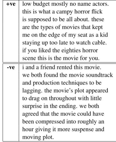
correctly classified by the discriminative BLSTM binary classifier, however they are correctly clas-sified by the cBLSTM LM classifier. We can ob-serve the implicit indication of the writer’s attitude towards the movie which can not be easily cap-tured by simple approaches. In this case, learning a separate long-span bidirectional probability dis-tribution for each sentiment seems to help.

+ve low budget mostly no name actors. this is what a campy horror flick is supposed to be all about. these are the types of movies that kept me on the edge of my seat as a kid staying up too late to watch cable. if you liked the eighties horror scene this is the movie for you.

-ve i and a friend rented this movie. we both found the movie soundtrack and production techniques to be lagging. the movie’s plot appeared to drag on throughout with little surprise in the ending. we both agreed that the movie could have been compressed into roughly an hour giving it more suspense and moving plot.

Table 5: Examples of reviews correctly classified by the cBLSTM LM classifier.

9 Conclusions

combi-nation, we could achieve further performance im-provement indicating that both the generative and discriminative approaches are complementary in solving the sentiment analysis problem. More-over, we have introduced an efficient methodol-ogy based on perplexity calculation to partition the training data according to relative importance to the learning task. This partitioning methodol-ogy has been combined with a sub-sampling tech-nique to efficiently train the neural networks on large data. As a future work, we plan to investi-gate deeper cBLSTM as well as hybrid recurrent and convolutional models. Another direction is to experiment with pre-trained word vectors.

Acknowledgments

The research leading to these results has received funding from the European Unions Horizon 2020 Programme through the Research and Innovation Action #645378 (ARIA-VALUSPA), the Innova-tion AcInnova-tion #644632 (MixedEmoInnova-tions), as well as the German Federal Ministry of Education, Sci-ence, Research and Technology (BMBF) under grant agreement #16SV7213 (EmotAsS). We fur-ther thank the NVIDIA Corporation for their sup-port of this research by Tesla K40 GPU donation.

References

Tanel Alum¨ae and Mikko Kurimo. 2010. Efficient estimation of maximum entropy language models with N-gram features: an SRILM extension. In Proc. Interspeech Conference of the International Speech Communication Association, pages 1820– 1823, Makuhari, Chiba, Japan, September.

Ebru Arisoy, Abhinav Sethy, Bhuvana Ramabhad-ran, and Stanely Chen. 2015. Bidirectional re-current neural network language models for

auto-matic speech recognition. In Proc. IEEE

Interna-tional Conference on Acoustics, Speech, and Signal Processing, pages 5421–5425, Brisbane, Australia, April.

Lalit R. Bahl, Frederick Jelinek, and Robert L. Mer-cer. 1983. A maximum likelihood approach to

con-tinuous speech recognition. IEEE Transactions on

Pattern Analysis and Machine Intelligence, 5:179 – 190, March.

Maximilian Bisani and Hermann Ney. 2004. Bootstrap estimates for confidence intervals in ASR

perfor-mance evaluation. InProc. IEEE International

Con-ference on Acoustics, Speech, and Signal

Process-ing, volume 1, pages 409 – 412, Montreal, Canada,

May.

George E. Dahl, Ryan Prescott Adams, and Hugo Larochelle. 2012. Training restricted boltzmann

machines on word observations. In Proc.

Interna-tional Conference on Machine Learning, pages 679– 686, Edinburgh, Scotland, UK, June.

Xiaowen Ding, Bing Liu, and Philip S. Yu. 2008. A holistic lexicon-based approach to opinion mining. In Proc. International Conference on Web Search and Data Mining, pages 231–240, Palo Alto, Cali-fornia, USA, February.

Li Dong, Furu Wei, Ming Zhou, and Ke Xu. 2014. Adaptive multi-compositionality for recursive neu-ral models with applications to sentiment analysis. InProc. AAAI Conference on Artificial Intelligence, pages 1537–1543, Qu´ebec, Qu´ebec, Canada, July.

Li Dong, Furu Wei, Ke Xu, Shixia Liu, and Ming Zhou. 2016. Adaptive multi-compositionality for recursive

neural network models.IEEE/ACM Transactions on

Audio, Speech & Language Processing, 24(3):422– 431.

Volkmar Frinken, Alicia Forn´es, Josep Llad´os, and

Jean-Marc Ogier, 2012. Bidirectional Language

Model for Handwriting Recognition, pages 611– 619. Springer Berlin Heidelberg, Berlin, Heidel-berg.

Alex Graves, Abdel rahman Mohamed, and Geoffrey Hinton. 2013. Speech recognition with deep

re-current neural networks. In Proc. IEEE

Interna-tional Conference on Acoustics, Speech, and Sig-nal Processing, pages 6645 – 6649, Vancouver, BC, Canada, May.

Sepp Hochreiter and J¨urgen Schmidhuber. 1997.

Long short-term memory. Neural Computation,

9(8):1735 – 1780, November.

Yi Hu, Ruzhan Lu, Yuquan Chen, and Jianyong Duan. 2007a. Using a generative model for

senti-ment analysis. International Journal of

Computa-tional Linguistics & Chinese Language Processing, 12(2):107–126, June.

Yi Hu, Ruzhan Lu, Xuening Li, Yuquan Chen, and Jianyong Duan. 2007b. A language modeling

ap-proach to sentiment analysis. InProc. International

Conference on Computational Science, pages 1186– 1193, Beijing, China, May.

Nal Kalchbrenner, Edward Grefenstette, and Phil Blun-som. 2014. A convolutional neural network for

modelling sentences. In Proc. Annual Meeting of

the Association for Computational Linguistics, vol-ume 1, pages 655–665, Baltimore, MD, USA, June.

Stefan Kombrink, Tom´aˇs Mikolov, Martin Karafi´at, and Luk´aˇs Burget. 2011. Recurrent neural network based language modeling in meeting recognition. In Proc. Interspeech Conference of the International Speech Communication Association, pages 2877 – 2880, Florence, Italy, August.

Siwei Lai, Liheng Xu, Kang Liu, and Jun Zhao. 2015. Recurrent convolutional neural networks for text

classification. InProc. AAAI Conference on

Artifi-cial Intelligence, pages 2267–2273, Austin, Texas, USA, January.

Quoc V. Le and Tom´aˇs Mikolov. 2014. Distributed representations of sentences and documents. In Proc. International Conference on Machine

Learn-ing, pages 1188–1196, Beijing, China, June.

Phong Le and Willem Zuidema. 2015. Compositional distributional semantics with long short term

mem-ory. InProc. Joint Conference on Lexical and

Com-putational Semantics, pages 10–19, Denver, CO, USA, June.

Kun-Lin Liu, Wu-Jun Li, and Minyi Guo. 2012. Emoticon smoothed language models for twitter

sentiment analysis. In Proc. AAAI Conference on

Artificial Intelligence, pages 1678–1684, Toronto, Ontario, Canada, July.

Andrew L. Maas, Raymond E. Daly, Peter T. Pham, Dan Huang, Andrew Y. Ng, and Christopher Potts. 2011. Learning word vectors for sentiment

anal-ysis. In Proc. Annual Meeting of the Association

for Computational Linguistics, pages 142–150, Port-land, Oregon, USA, June.

Tom´aˇs Mikolov, Martin Karafi´at, Luk´aˇs Burget, Jan H. ˇCernock´y, and Sanjeev Khudanpur. 2010.

Recur-rent neural network based language model. InProc.

Interspeech Conference of the International Speech Communication Association, pages 1045 – 1048, Makuhari, Chiba, Japan, September.

Bo Pang and Lillian Lee. 2004. A sentimental educa-tion: Sentiment analysis using subjectivity

summa-rization based on minimum cuts. In Proc. Annual

Meeting of the Association for Computational Lin-guistics, pages 271 – 278, Barcelona, Spain, July. Bo Pang, Lillian Lee, and Shivakumar Vaithyanathan.

2002. Thumbs up?: Sentiment classification using

machine learning techniques. In Proc. Conference

on Empirical Methods in NLP, volume 10, pages 79–86, Philadelphia, PA, USA, July.

´Alvaro Peris and Francisco Casacuberta. 2015. A bidi-rectional recurrent neural language model for

ma-chine translation. Procesamiento del Lenguaje

Nat-ural, 55:109–116, September.

Wenge Rong, Baolin Peng, Yuanxin Ouyang, Chao Li, and Zhang Xiong. 2014. Structural information aware deep semi-supervised recurrent neural

net-work for sentiment analysis. Frontiers of Computer

Science, 9(2):171–184.

C´ıcero Nogueira dos Santos and Maira Gatti. 2014. Deep convolutional neural networks for sentiment

analysis of short texts. InProc. International

Con-ference on Computational Linguistics, pages 69–78, Dublin, Ireland, August.

Bj¨orn Schuller, Amr E. Mousa, and Vryniotis Vasileios. 2015. Sentiment analysis and opin-ion mining: On optimal parameters and

perfor-mances. WIREs Data Mining and Knowledge

Dis-covery, 5:255–263, September/October.

Richard Socher, Alex Perelygin, Jean Y. Wu, Jason Chuang, Christopher D. Manning, Andrew Y. Ng, and Christopher Potts. 2013. Recursive deep mod-els for semantic compositionality over a sentiment

treebank. InProc. Conference on Empirical

Meth-ods in NLP, pages 1631–1642, Seattle, WA, USA, October.

Andreas Stolcke. 2002. SRILM - an extensible

lan-guage modeling toolkit. InProc. International

Con-ference on Spoken Language Processing, volume 2, pages 901 – 904, Denver, Colorado, USA, Septem-ber.

Martin Sundermeyer, Ralf Schl¨uter, and Hermann Ney. 2012. LSTM neural networks for language

model-ing. InProc. Interspeech Conference of the

Inter-national Speech Communication Association, Port-land, OR, USA, September.

Maite Taboada, Julian Brooke, Milan Tofiloski, Kim-berly Voll, and Manfred Stede. 2011.

Lexicon-based methods for sentiment analysis.

Computa-tional linguistics, 37(2):267–307, June.

Kai Sheng Tai, Richard Socher, and Christopher D. Manning. 2015. Improved semantic representa-tions from tree-structured long short-term memory

networks. In Proc. Annual Meeting of the

Associ-ation for ComputAssoci-ational Linguistics, pages 1556– 1566, Beijing, China, July.

Sida I. Wang and Christopher D. Manning. 2012. Baselines and bigrams: Simple, good sentiment and

topic classification. InProc. Annual Meeting of the

Association for Computational Linguistics, pages 90 – 94, Jeju Island, Korea, July.

Felix Weninger, Johannes Bergmann, and Bj¨orn Schuller. 2014. Introducing CURRENNT – the Munich open-source CUDA RecurREnt Neural

Net-work Toolkit. Journal of Machine Learning

Re-search, 15(99), October.