Bayesian Estimation of Defect Inspection Cycle Time in TFT-LCD Module Assembly Process

Bayesian Estimation of Defect Inspection Cycle

Time in TFT-LCD Module Assembly Process

Chien-wen Shen

Abstract—The defect inspection station is one of the major

processes in module assembly stage of TFT-LCD panel manufacturing. Because this process is usually examined manually through human vision, its cycle time estimation is more uncontrollable and therefore could easily affect the customer response time. Hence, this study would like to apply Bayesian networks approach to establish a reliable cycle time prediction model for this key procedure. Our initial model includes work-in-process, throughput, yield, and number of product mixes as the possible explanatory drivers of defect inspection cycle time. To validate the applicability of proposed model, structural and parameter learning is further performed through the data of a TFT-LCD manufacturing plant. Our findings not only demonstrate the feasibility of Bayesian approach in cycle time estimation but also prove its prediction quality by comparing to the results from discriminant analysis.

Index Terms—Cycle time, Bayesian networks, Discriminant

analysis.

I. INTRODUCTION

Due to the growing demand of light, thin, and power-saving electronic products, the development of TFT-LCD (Thin Film Transistor - Liquid Crystal Display) industry is prosperous in today’s digital broadcasting age. According to the study of DisplaySearch, global LCD television shipments exceed 54 million sets in 2006. As more countries switch off analog broadcasting services in the near future, the explosive needs of TFT-LCD panels can be expected. Generally speaking, TFT–LCD panel is primarily used as a display instrument for computers or consumer electronics. Meanwhile, its flat panel displays (FPD) could also be applied in other technology solutions [2]. Comparing to the traditional cathode ray tube (CRT) technology, TFT-LCD panel is light and small in size. In addition, it flickers less, consumes less power, and does not produce electromagnetic radiation. Principal TFT-LCD components include polarizing filter, glass substrate, transparent electrodes, alignment layer, liquid crystal, spacer, color filter, backlighting, etc [11]. Its manufacturing requires sophisticated upstream industries including glass substrate, backlight module, color filter, polarizer, flexible print circuit, driver IC, printed circuit board, and chemical to support the whole TFT-LCD supply chain [8].

The manufacturing of TFT-LCD is basically composed of three key processes: array, cell, and module. In the module

assembly process, panels go through crucial procedures such as chip on glass, printed circuit board (PCB), PCB inspection, silicon dispenser, assembly, and defect inspection to complete the final products. Among the above mentioned processes in module assembly, defect inspection is likely becoming the bottleneck for customer response time due to its characteristics of manual operations. Operators in defect inspection station commonly have to visually examine the electrical specifications, appearance specifications, and outside dimension of panels. For example, there should be less than 8 bright dots and 8 dark dots under the panel inspection of electrical specifications. Besides, the total dots defects should be less than 12 dots [3]. Operators have to use naked eyes through the assistance of neutral density filter to discriminate display mura from the samples based on the agreement between the manufacturer and customer [10]. Moreover, operators have to examine active area, bezel, label, solder, screw, white sheet, connector, and flexible print circuit board for appearance specification and dimension, weight, display tolerance, and panel gap for outside dimension check. Although there have been developed machine-operated methods for specific types of panel defects [10][12][15][20], most manufacturers still ask the operators to use the images produced from pattern generator, video board, or luminance colorimeter to visually detect panel flaws. As a result, cycle time estimation of defect inspection is unlikely to be provided by manufacturing execution system and is generally determined by experienced practitioners. However, their cycle time estimates on defect inspection are generally unreliable and could cause delay on delivery response time. Hence, this study would like to investigate how to develop a dependable prediction model for this particular manual- operated procedure to avoid the drawbacks of human assessment.

The approach of Bayesian networks (BNs) was applied to construct the cycle time estimation model because of its modeling advantages in graphical representation and learning capability. Because Bayesian network model requires the specifications of dependent variables for defect inspection cycle time, related variables are explored in section 2. Details of model construction from BNs methodology is then described in section 3. To validate the applicability of our proposed model, a TFT-LCD panel factory was selected as our case study. Based on the data collected from this sample factory, results of structural learning, parameter learning and statistical inference are later investigated in section 4. Prediction quality of BNs is also compared with the findings from discriminant analysis. In the final section, conclusions about BNs approach for defect inspection cycle time in TFT-LCD industry are addressed.

II. PREDICTORS OF CYCLE TIME ESTIMATION

Although studies regarding the estimation of defect inspection cycle time are limited, we tried to understand the potential predictor variables of our research interest through the literature review of cycle time prediction in the electronic industry. For example, Srivarsan and Kempf [18] described an effective approach to throughput time modeling in a semiconductor wafer fabrication facility. They found out that process time, transport time, variable availability of resource, machine and operator dedications, non-product lots, batching and setups, work-in-process (WIP) management policies, lots on hold and rework lots are significant contributors to factory throughput time. Zargar [21] developed an equation that is composed of machine setup time, number of wafers in a lot, process time, rework time, and probability that a wafer fails to compute the expected lot cycle time. Raddon and Grigsby [16] constructed an estimation model for throughput time. They considered utilization over availability, theoretical throughput time, number of tools, and number of steps in line as the potential factors of throughput time. Besides, they also approximated step cycle time by the variability of arrival and processing time, average step cycle time, utilization, and number of machines. Lee et al. [14] introduced a linear programming model for wafer production planning in semiconductor wafer fabrication. The objective of this model is to optimize the behaviors of cycle time and the level of WIP in order to satisfy the due dates of demand under the capacity constraints of capacitated loading procedure. Through the understanding of their planning model, factors like capacity, WIP, and cycle time are critical in the consideration of wafer production planning. Study from Sivakumar and Chong [17] applied a data driven discrete event simulation model to discuss the relationship between input variables and output variables in semiconductor backend manufacturing system. Features like preventative maintenance schedules, yield information, rework, units per hour, batch process time, down time, shift pattern, set-up time matrix and product mix variety are taken into account in their model. Findings of this study can help to control input variables for cycle time reduction.

Additionally, Haberle and Graves [5] investigated the cycle time estimation models for design stage, resource planning stage, and manufacturing stage of printed circuit board. Variables of redesign, in-circuit test, and board type are used for the prediction of design phase cycle time. Meanwhile, they considered board type, number of signal layers, and part lead form as the potential drivers of cycle time in resource planning phase. In the stage of manufacturing, board function and number of layers are correlated to cycle time assessment. Their mathematical model of total cycle time includes board function, component, redesign, and in-circuit test as the predictor variables. Hung and Chang [7] experimented exponential smoothing method and iterative empirical curve approach to predict flow time in dispatch rules. Findings indicate that the hours of a small time period, number of machine in work station, the total workload arrival to work station, the queue amount of work station, the capacity of work station, and the loading rate of work station are highly related to the flow time prediction under the iterative empirical curve approach. Chung and

Huang [4] analyzed the characteristics of material flow for a wafer fab and then developed its corresponding algorithms for cycle time estimation. Findings show that their algorithm is able to provide reliable cycle time estimations with or without existing engineering lots. Haller, Peikert, and Thoma [6] discussed how to manage cycle time through WIP control and monitoring. Findings implied that yield, product qualification, and equipment qualification could be directly influenced by cycle time. Finally, Beeg [1] also describes how to predict future wafer fab cycle time. Related data such as equipment uptime, equipment utilization, number of process steps running in the work center, process speed, theoretical fastest cycle time per step, current cycle time per step, number of tools, and number of processed wafers are used for cycle time estimation. According to the above literature review, various factors of cycle time predictions are examined in different situations of manufacturing processes. Although there are little studies addressed the issue of defect inspection cycle time, the above mentioned variables could be the potential drivers of our research interest. Hence, next section will describe how to select the suitable explanatory variables for the cycle time estimation model of defect inspection.

III. CONSTRUCTION OF BAYESIAN MODEL

Instead of using the techniques such as data-driven (activity-based), simulation, queuing theory, regression analysis, or hybrid approach mentioned in section 2, we applied Bayesian networks methodology to construct an estimation model for defect inspection cycle time. BN is a reasoning approach that has many advantages that other techniques do not have. For example, we can use observed knowledge to validate the graphical representation of BN model even if we were unsure about the relationships among variables. Conditional probabilities can be also updated through the collection of new data even if the prior beliefs are unreliable. Besides, BN is able to handle incomplete data or different data types without further assumptions or adjustments. As some of the cycle time estimation methods mentioned above may need detailed information on corresponding procedures and parameters, Bayesian networks on the other hand can handle those problems through parameter learning or structural learning from accumulating data. Because we do not have strong prior knowledge regarding model structure or conditional probabilities, BN approach is suitable for our research situations.

Formally, BN is composed of qualitative and quantitative configurations. A directed acyclic graph with nodes and directed arcs has to be specified at qualitative stage of BN construction. Nodes in BN models denote variables of interests. Arcs between nodes imply conditional dependences among variables. At quantitative level, beliefs are represented by conditional probability distributions. Here in this section, we start with the discussion of qualitative construction of BN model. Then the development of quantitative specification and statistical inference based on the data collected from a TFT-LCD panel factory is discussed later in section 4.

factors that might affect the defect inspection cycle time have to be identified first. Due to the manual operation nature of defect inspection in TFT-LCD manufacturing, cycle times of individual inspection procedures are generally short and operator-dependent. Data for corresponding activities within defect inspection station is therefore hard to collect. To resolve this situation, data of preceding stations that can be retrieved from manufacturing execution systems becomes the candidates of cycle time predictors. Under the assumptions that the outputs of operators have no significant differences, the volume and complexity of products before entering the defect inspection station may affect the performance of inspection. Hence, according to the literature review in section 2, estimation model of this study only includes WIP in previous period, throughput in previous period, yield in previous period, and number of product mixes in current period as the predictor variables of defect inspection cycle time. Weekly data is considered in order to be consistent with the interval of scheduling and planning in TFT-LCD plants. Consequently, direct arcs are drawn from these predictor nodes to the node of cycle time in our graphical model. These arcs illustrates that cycle time is dependent on predictor variables WIP, throughput, yield and product mixes. Figure 1 demonstrates the initial relationships among variables based on our model assumptions. This conceptual model is used to estimate the defect inspection cycle time from the perspectives of Bayesian theories. Although there is no prior knowledge regarding these relationships, structural learning of BNs can be adopted for further removal or addition of corresponding arcs. Algorithm of necessary path condition (NPC) was applied for structural learning in this study [19]. Because probabilities are used to encode beliefs or uncertain events in BNs at quantitative level, we also applied expectation-maximization (EM) algorithm [13] to use collected data to estimate the conditional probability distributions of our estimation model. To make inference through BN model, this study utilized the probability updating algorithm from Jensen, Lauritzen, and Olesen [9] to compute the conditional probabilities of variables given the evidence on other variables. Because conditional probabilities are used to make inference from Bayesian perspectives, the conditional probabilities of explanatory variables given the evidences of cycle time and the conditional mean of cycle time given the evidences of explanatory variables are computed in this study to analyze the behavior of defect inspection cycle time.

Figure 1: Bayesian Model for Cycle Time Estimation

IV. PRACTICAL APPLICATION

Based on the proposed model described in section 3, model applicability was tested against a TFT-LCD manufacturing plant. A total of 91 weekly data regarding cycle time, work-in-process, throughput, yield, and number of product mixes was retrieved from manufacturing execution systems of the plant. Each variable is categorized into 4 conditions for practical explanation. For example, cycle time is classified into (1) less than 6 hours, (2) between 6 hours and 12 hours, (3) between 12 hours and 18 hours, and (4) more than 18 hours. The other predictor variables are categorized into (1) low, (2) medium-low, (3) medium-high, and (4) high. These definitions of classifications are specified by plant engineers to accord with on-site requirements. In the following discussion, findings of structural learning and parameter learning of our BN model based on the data of six seasons are described first in subsection A. After completing the qualitative and quantitative specifications of BN model through data learning, results of inference and estimation are discussed in subsection B. We applied one season of data to analyze the prediction quality of BN approach. Estimation results of BN model were also compared with the ones from discriminant analysis.

A. Structural and Parameter Learning

In order to construct a reliable model for estimation, learning mechanism was applied upon the original conceptual model. According to NPC algorithm, result of structural learning is depicted in Figure 2, where original arcs are still remained in the new model. It indicates that our initial dependent assumptions regarding cycle time and predictor variables are consistent with actual observations. Besides, an additional arc drawing from “Product Mix” to “Yield” after structural learning represents the conditional dependent of “Yield” on “Product Mix” from accumulating data. This minor adjusted model is later used for parameter learning and cycle time prediction.

Figure 2: Bayesian Model after Structural Learning After constructing the qualitative level of BN model, EM algorithm was applied to perform parameter learning for updating probabilities. Because joint probabilities are difficult to represent in tabular format, marginal probabilities after parameter learning are shown in Table 1. In terms of mathematical expression, cells in Table 1 demonstrate the results of probabilities P(Variable = i | Data of 6 seasons),

where i = 1,2,3,4. For example, the marginal probabilities of

cycle time = i given the data of 6 seasons are 0.3396, 0.3717,

0.1626 and 0.1259 for i = 1, 2, 3, and 4 respectively. It means

that around 70% of defect inspection cycle time is less than Throughput

WIP

Yield

Cycle Time

Throughput WIP

Cycle Time

Yield Product Mix

12 hours. Meanwhile, the posterior marginal probability of WIP = “Medium-Low” is 0.5385, which is significantly higher than the other conditions of WIP. For the predictor variables of throughput and yield, around 70% of the conditions occur in “Medium-Low” or “Medium-High”. On the other hand, the probabilities of product mix are almost evenly distributed for each condition. These posterior marginal probabilities can help us understand the likely distributions of variables. In addition, the following inference discussion is based on the joint probabilities after EM learning algorithm for the corresponding variables in our proposed estimation model.

Table 1: Marginal Probabilities after Parameter Learning 1 2 3 4 Cycle Time 33.96 37.19 16.26 12.59

WIP 21.79 53.85 15.38 8.97

Throughput 19.23 37.18 32.05 11.54

Yield 14.10 33.33 39.74 12.84

Product Mix 20.51 34.62 23.08 21.79 Unit: %

B. Statistical Inference

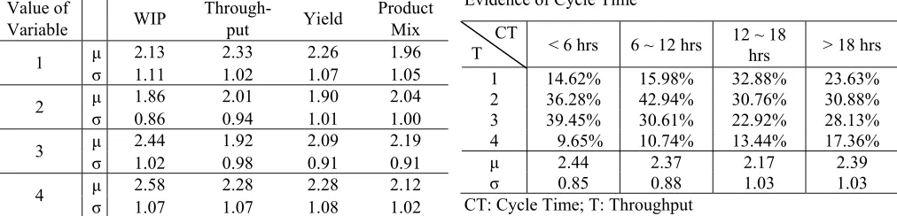
From the view point of Bayesian approach, the conditional probabilities given evidence can be used to make statistical inference. Thus in this study, the estimation of cycle time is analyzed through different angles of probability distributions. We start with the discussion of expected cycle time given the conditions of respective variables. Findings of expected cycle time are summarized in Table 1, where the mean (μ) and standard deviation (σ) of cycle time given the evidence of predictor variables are calculated by updating algorithm from Jensen, Lauritzen, and Olesen [9]. According to the results of column WIP in Table 1, expected cycle time has highest value of 2.58 when WIP is observed as “High” and lowest value of 1.86 when WIP is observed as “Medium-Low”. But the mean differences between various conditions of predictor variables are smaller than 0.5 for throughput, yield, and product mix. It implies that the expected difference of defect inspection cycle time is less than 3 hours given any evidence from these three predictor variables. In addition, findings from Table 1 also suggest that expected cycle time is around “2", which indicates the expected cycle time is more likely less than 12 hours but higher than 6 hours given any evidence from individual predictor variable. Staff of defect inspection station could refer this value for customer response time under the situation of limited available information.

Table 1: Expected Cycle Time Given the Value of Predictor Value of

Variable WIP

Through-put Yield

Product Mix

1 μ 2.13 2.33 2.26 1.96

σ 1.11 1.02 1.07 1.05

2 μ 1.86 2.01 1.90 2.04

σ 0.86 0.94 1.01 1.00

3 μ 2.44 1.92 2.09 2.19

σ 1.02 0.98 0.91 0.91

4 μ 2.58 2.28 2.28 2.12

σ 1.07 1.07 1.08 1.02

To analyze cycle time behavior from Bayesian perspective, we can also compute the posterior probability of predictor variable given the evidence of cycle time. Let’s consider the situation of WIP first. Suppose the observed evidence of cycle time is less than 6 hours, posterior probabilities of WIP = “Low”, “Medium-Low”, “Medium-High”, and “High” are 0.2475, 0.6038, 0.9130, and 0.5740 respectively according to Table 2. It implies that the volume of WIP is likely in “Medium-Low” level when observed cycle time is less than 6 hours. Similar situation happens when the evidence of cycle time is between 6 hours and 12 hours. Although WIP = “Medium-Low” still has the highest probability when observed cycle time is between 12 and 18 hours, the probability distribution is spread over the other values of WIP. Table 2 also indicates that the probabilities of WIP are more evenly distributed and the standard deviation (σ) of WIP is higher as the observed cycle time is getting higher. However, we are unable to have a better understanding of cycle time performance from the expected values (μ) of WIP given the evidence of cycle time because their differences are not significant.

Table 2: Posterior Probability of WIP Given the Evidence of Cycle Time

CT

W < 6 hrs 6 ~ 12 hrs 12 ~ 18 hrs > 18 hrs 1 24.75% 15.73% 23.19% 29.94% 2 60.38% 64.42% 35.33% 28.89% 3 9.13% 14.61% 23.05% 24.64% 4 5.74% 5.24% 18.43% 16.53% μ 1.96 2.09 2.37 2.28

σ 0.75 0.71 1.03 1.06

CT: Cycle Time; W: WIP

Next, let’s discuss the situation of throughput. Table 3 summarizes the posterior probabilities of throughput given the evidence of cycle time. When the observed evidence of cycle time is less 12 hours, the total posterior probability of

P(Throughput = “Medium-Low” | Cycle Time = 6 hours or

6~12 hours) and P(Throughput = “Medium-High” | Cycle

Time = 6 hours or 6~12 hours) is close to 75%. Similarly like the situation of WIP, the standard deviation (σ) of throughput is getting higher and the probability distribution of throughput is more dispersed over the possible values of cycle time as the observed cycle time increases. Meanwhile, the differences among the expected values of throughput given the evidence of cycle time are still small.

Table 3: Posterior Probability of Throughput Given the Evidence of Cycle Time

CT

T < 6 hrs 6 ~ 12 hrs 12 ~ 18 hrs > 18 hrs 1 14.62% 15.98% 32.88% 23.63% 2 36.28% 42.94% 30.76% 30.88% 3 39.45% 30.61% 22.92% 28.13% 4 9.65% 10.74% 13.44% 17.36% μ 2.44 2.37 2.17 2.39

σ 0.85 0.88 1.03 1.03

The probability distribution of yield given the evidence of defect inspection cycle time is a little different than the distributions of previous discussion. According to the results of Table 4, the posterior probability distribution of throughput given the evidence of cycle time = ‘3’ or ‘4’ is slightly more centralized than the ones from WIP and throughput. In the meantime, the standard deviation of yield is smallest and the posterior probability of yield = ‘Medium-High” is as high as 50% when the observed cycle time is between 6 to 12 hours.

Table 4: Posterior Probability of Yield Given the Evidence of Cycle Time

CT

Y < 6 hrs 6 ~ 12 hrs 12 ~ 18 hrs > 18 hrs 1 12.76% 11.46% 18.97% 19.27% 2 44.39% 27.53% 25.79% 30.39% 3 31.42% 50.88% 37.85% 31.73% 4 11.43% 10.13% 17.39% 18.61% μ 2.42 2.60 2.54 2.50

σ 0.85 0.82 0.99 1.00

CT: Cycle Time; Y: Yield

For the situation of product mix, Table 5 illustrates the posterior probabilities of product mix given the evidence of cycle time. Because all of the standard deviations of product mix given evidence are larger than 1, we can expect the probability distributions of product mix given the evidences of cycle time are more evenly spread over the possible values of product mix comparing to the results from WIP, throughput, and yield. The findings from Table 2 to Table 5 can help us to understand the posterior probability distributions of predictor variables given the evidence of defect inspection cycle time.

Table 5: Posterior Probability of Product Mix Given the Evidence of Cycle Time

CT

P < 6 hrs 6 ~ 12 hrs 12 ~ 18 hrs > 18 hrs 1 26.31% 16.40% 17.08% 21.45% 2 37.45% 32.70% 33.84% 33.63% 3 15.36% 29.16% 27.29% 20.48% 4 20.88% 21.74% 21.79% 24.44% μ 2.31 2.56 2.54 2.48

σ 1.08 1.00 1.01 1.08

CT: Cycle Time; P: Product Mix

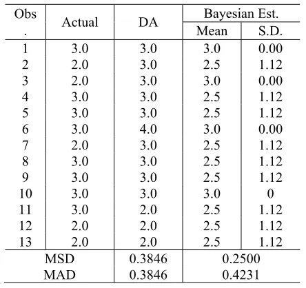
Finally, data of one season is used to evaluate the prediction quality of our proposed Bayesian model. Table 6 demonstrates the expected values and standard deviations of defect inspection cycle time based on the model and probability distributions after structural learning and parameter learning. Due to the characteristic of Bayesian approach, expected cycle time is computed and therefore their corresponding estimations do not commonly match the exact values of classification codes. But the staff is still able to provide an estimation of cycle time based on the observations of predictor variables. For example, the actual cycle time of observation 2 is “2”, which denote the cycle

time ranging from 6 hours to 12 hours. The estimation from our BN model is 2.5, which suggests the expected cycle time could be “between 6 to 12 hours” or “between 12 to 18 hours”. Comparing the estimation results of BN model with the ones from discriminant analysis, Table 6 shows that the mean square deviation of BN model is less than the one of discriminant analysis. Alternatively, the mean absolute deviation has opposite outcome for discriminant analysis and BN model. Hence, we can conclude that the estimation quality of BN approach is at least as good as the result of discriminant analysis according to the observations of sample TFT-LCD plant.

Table 6: Comparisons of Cycle Time Estimations between Discriminant Analysis and Bayesian Model

Obs

. Actual DA

Bayesian Est. Mean S.D. 1 3.0 3.0 3.0 0.00 2 2.0 3.0 2.5 1.12 3 2.0 3.0 3.0 0.00 4 3.0 3.0 2.5 1.12 5 3.0 3.0 2.5 1.12 6 3.0 4.0 3.0 0.00 7 2.0 3.0 2.5 1.12 8 3.0 3.0 2.5 1.12 9 3.0 3.0 2.5 1.12 10 3.0 3.0 3.0 0 11 3.0 2.0 2.5 1.12 12 2.0 2.0 2.5 1.12 13 2.0 2.0 2.5 1.12 MSD 0.3846 0.2500 MAD 0.3846 0.4231 DA: Discriminant Analysis; S.D.: Standard Deviation;

Obs.: Observation; MSD: Mean Square Deviation; MAD: Mean Absolute Deviation

V. CONCLUSIONS

BN model. In addition to discriminant analysis, we may further compare BN approach with the other methodologies in order to understand the advantages or disadvantages of respective methods in the issues of cycle time estimation for manually operated processes in TFT-LCD panel manufacturing.

REFERENCES

[1] T. Beeg, “Wafer fab cycle forecast under changing loading situations,”

Proceedings of IEEE 2004 Advanced Semiconductor Manufacturing,

pp. 339-343, 2004.

[2] S. C. Chang, “The TFT-LCD industry in Taiwan: competitive advantages and future developments,” Technology in Society, vol. 27, pp. 199-215, 2005.

[3] T. Chen, Incoming Inspection Specification for 23” TFT-LCD

Modules, AU Optronics Corp., 2006.

[4] S. H. Chung, and H. W. Huang, “Cycle time estimation for wafer fab with engineering lots,” IIE Transactions, vol. 34, no. 2, pp. 105-118, 2002.

[5] K. R. Haberle, and R. J. Graves, “Cycle time estimation for printed circuit board assemblies,” IEEE Components, Packaging and

Manufacturing Technology, vol. 24, no. 3, pp. 188-194, 2001.

[6] M. Haller, A. Peikert, and J. Thoma, “Cycle time management during production ramp-up,” Robotics and Computer Integrated

Manufacturing, vol. 19, pp. 183-188, 2003.

[7] Y. F. Hung, and C. B. Chang, “Dispatching rules using flow time predictions for semiconductor wafer fabrications,” Journal of the Chinese Institute of Industrial Engineers, vol. 19, no. 1, pp. 67-74, 2002.

[8] Industrial Technology Research Institute (ITRI), 2002 Annual Report

of Flat Panel Display Industry, ITRI, Hsinchu, Taiwan, 2002.

[9] F. V. Jensen, S. L. Lauritzen, and K. G. Olesen, “Bayesian updating in causal probabilistic networks by local computations,” Computational Statistics Quarterly, vol. 4, pp. 269-282, 1990.

[10] B. C. Jiang, C. C. Wang, and H. C. Liu, “LCD surface uniformity defect inspection using ANOVA and EWMA techniques,’ International

Journal of Production Research, vol. 43, no. 1, pp. 67-80, 2005.

[11] M. Katayama, “TFT-LCD technology,” Thin Solid Films, vol. 341, pp. 140-147, 1999.

[12] J. H. Kim, S. Ahn, J. W. Jeon, and J. E. Byun, “A high-speed high-resolution vision system for the inspection of TFT LCD,”

Proceedings of the ISIE 2001 IEEE International Symposium, vol. 1,

pp. 101 –105, 2001.

[13] S. L. Lauritzen, “The EM algorithm for graphical association models with missing data,” Computational Statistics & Data Analysis, vol. 19, pp. 191-201, 1995.

[14] Y. Lee, S. Kim, S.Yea, and B. Kim, “Production planning in semiconductor wafer fab considering variable cycle times,” Computers & Industrial Engineering, vol. 33, no. 12, pp. 713-716, 1997. [15] C. J. Lu, D. M. Tsai, and H. N. Yen, “Automatic defect inspection for

LCDs using singular value decomposition,” Proceedings of the Fourth Asia-Pacific Conference on Industrial Engineering and Management

Systems, 2002. (CD-ROM)

[16] A. Raddon, and B. Grigsby, “Throughput time forecasting model,” Proceedings of the 1997 IEEE/SEMI Advanced Semiconductor

Manufacturing Conference and Workshop, pp. 430- 433, 1997.

[17] A. I. Sivakumar, and C. S. Chong, “A simulation based analysis of cycle time distribution, and throughput in semiconductor backend manufacturing,” Computers in Industry, vol. 45, no. 1, pp. 59-78, 2001.

[18] N. Srivatsan, and K. Kempf, “Effective modeling of factory throughput times,” IEEE/CPMT. International Electronics Manufacturing

Technology Symposium, pp. 377–383, 1995.

[19] H. Steck, Constrained-Based Structural Learning in Bayesian

Networks Using Finite Data Sets, PhD Thesis, Institut für der

Informatik der Technischen, 2001.

[20] M. H. Wu, C. S. Fuh, and H. Y. Chen, “Defect inspection and analysis of color filter panel,” Image and Recognition, vol. 6, no. 2, pp. 74-90, 2000.

[21] A. Zarger, “Effect of rework strategies on cycle time,” Computers and