Online Full Text

Abstract—This paper investigates the application of

multi-sensor data fusion (MSDF) technique to enhance the process fault detection and diagnosis. The Extended Kalman Filter (EKF) is used to fuse the process measurement sensor data. The usual approach in the classical EKF implementation, however, is based on the constant diagonal matrices for the process and measurement covariance. This inflexible constant covariance set-up which employs the ideal white noise model assumption for describing the process and measurement noises causes the EKF algorithm to diverge or at best converge to a large bound even it the EKF model is perfectly tuned. This paper presents an adaptive modified extended kalman filter (AMEKF) algorithm based on the fuzzy logic idea to prevent the filter divergence leading to an improved EKF estimation. The performances of the resulting fault detection and diagnosis system are demonstrated an a simulated continuous stirred tank reactor( CSTR) benchmark case study for single, double, triple and quadruple faults.

Index Terms— Faults Detection and Diagnosis, Multi-sensor

data fusion, Adaptive Modified Extended Kalman Filter, Fuzzy Logic

I. INTRODUCTION

Associated with an increasing demand for high performance as well as for more safety and reliability of dynamic systems, and a natural trend toward system automation, fault detection and diagnosis has received more and more attention. The existing techniques for fault detection and diagnosis can be broadly divided into process history based and process model-based methods. Each of these can further be classified into qualitative and quantitative approaches. The qualitative approaches involve fault trees [1], signed directed graph [2], fuzzy logic [3], neural networks [4], and expert systems [5], The quantitative approaches are basically modeling, filtering

Manuscript received July 22, 2007.

M. Mosallaei is with the Automation and Instrumentation Department Petroleum University of Technology (PUT), Tehran, Iran (e-mail: mohsenmosallaei@ gmail.com).

K. Salahsoor is with the Automation and Instrumentation Department, Petroleum University of Technology (e-mail: [email protected]).

M. R. Bayat is with the Automation and Instrumentation Department, Petroleum University of Technology (e-mail: [email protected]).

K. Amanian is with the Automation and Instrumentation Department, Petroleum University of Technology (e-mail: amaniankarim@ gmail.com).

and estimation methods, where a wide variety of them have already been reviewed by [6]-[7]-[8]. Among the existing quantitative model-based methods, the Kalman filter variants have found widespread applications.

In this paper, multi-sensor data fusion (MSDF) technique is used to improve the accuracy of the process fault detection and diagnosis. The field of multi-sensor data fusion is fairly young which has mainly been considered and developed in military target tracking and autonomous robotics. This technique seeks to combine data from multiple sensors and related information to achieve improved accuracies and more specific inferences than could be achieved by using a single and independent sensor. Thus, the main problem is focused on the methodology by which the multi-sensor measurements can be combined and processed to obtain a joint state-vector estimation which is better than the individual sensor-based estimates. There are various multi-sensor data fusion approaches to resolve this problem, of which the Kalman filtering is the most significant one. Methods for Kalman-filter-based data fusion, including state-vector fusion and measurement fusion, have been widely studied over the last decade. Also, we are using of extended kalman filter technique for fault detection and diagnosis. In the actual implementation of the kalman filter, the measurement noise covariance is usually measured prior to operation of the filter. Measuring the measurement error covariance is generally practical (possible) because we need to be able to measure the process anyway (while operating the filter) so we should generally be able to take some off-line sample measurements in order to determine the variance of the measurement noise. The determination of the process noise covariance Q is generally more difficult as we typically do not have the ability to directly observe the process we are estimating. Sometimes a relatively simple (poor) process model can produce acceptable results if one “injects” enough uncertainty into the process via the selection of Q. Certainly, in this case one would hope that the process measurements are reliable. In either case, whether or not we have a rational basis for choosing the parameters, often superior filter performance (statistically speaking) can be obtained by tuning the filter parameters Q and R. The tuning is usually performed off-line, frequently with the help of another (distinct) Kalman filter in a process generally referred to as system identification. Under conditions where Q and R are in fact constant, both the estimation error covariance Pk and the

Process Faults Diagnosis with Multi-sensor Data

Fusion Architecture Based on Adaptive

Extended Kalman Filters and Fuzzy Logic

Kalman gain Kkwill stabilize quickly and then remain constant.

If this is the case, these parameters can be pre-computed by either running the filter off-line, or for example by determining the steady-state value of Pkas described in [9]. It is frequently

the case however that the measurement error (in particular) does not remain constant. Also, the process noise is sometimes changed dynamically during filter operation (becoming Qk) in

order to adjust to different dynamics. In such cases time-varying covariance might be chosen to account for both uncertainties about the user’s intentions and uncertainty in the model.

Therefore, in real application, the exact values of Qk and Rk

are not known. If the actual process and measurement noises are not zero-mean white noises, the residual in the extended Kalman filter will also not be a white noise. If this is happened, the Kalman filter would diverge or at best converge to a large bound. This paper investigates the usefulness of the fuzzy logic method to improve the accuracy of the state estimation procedure done by the MEKF algorithm for the process fault detection and diagnosis purposes.

The remainder of this paper is organized as follows. In section II, the proposed methodology is presented. Section III describes the CSTR case study plant. The effectiveness of the proposed approach is demonstrated in section IV. Finally, the conclusions are given in section V.

II. PROPOSED METHODOLOGY

A. Extended kalman filtering algorithm

The Kalman filter [10] provides an efficient recursive procedure to estimate the hidden states x∈Rnxof a discrete-time process that is governed by the linear stochastic process and measurement model equations:

1

1 −

−

+

+

=

_{k k k}

k

Ax

Bu

w

x

(1)

k k

k

Hx

v

z

=

+

(2) where xk denotes the hidden states, uk∈Rnu is the vector of

external manipulated input variables, and zk∈Rnzrepresents the

vector of noisy measured output variables at the kth discrete time. The random variables wk-1 and vk represent the process

and measurement noises, respectively. A is the state transition matrix, B is the control matrix and H is the output observation matrix. However, in most practical applications of interest, the process dynamics and the measurement equations obey the following non-linear relationships:

1

1

,

,

)

(

−

+

−

=

_{k k k}

k

f

x

u

k

w

x

(3)

k k

k

h

x

k

v

z

=

(

,

)

+

(4) where f and h are known nonlinear functions. As a result, nonlinearity can come in either through process model and/or through the measurement model. Applying the standard Kalman filter on the linearized process and measurement equations about the nominal state values can introduce large errors leading to sub-optimal filter performance.

EKF gives a simple and effective remedy to overcome such

problem. Its basic idea is to locally linearize the non-linear system described by (3) and (4) at each time instant around the most recent state estimate and then the Kalman filter is applied to the resulting time-varying linearized model. This can provide a more accurate implementation of the optimal recursive estimation procedure.

B. Discrete-time modified extended Kalman filter

In practice, the process model in (3) is of continuous-time nature. While, the measurements in (4) are available through the common digital data-acquisition systems at discrete measurement time instants. Moreover, the EKF algorithm is implemented digitally to process all available measurements regardless of their precision in order to provide a quick and accurate estimate of the variables of interest. Therefore, an efficient formulation of the algorithm needs to be made for a real-time practical application to minimize the filter cycle time, while obtaining a reasonable accuracy in the filter implementation. The method used in this paper for numerical integration of the process model from one sample time to the next is the first-order Euler integration technique. The time propagation equation for the state covariance matrix P can be solved using the transition matrix technique [11]. This method preserves both the symmetry and the positive definiteness of P, and yields adequate performance:

d T k

k

P

Q

P

−

=

Φ

₋

Φ

+

1 (5)

Where Ts is the sampling period and

∫

−

Φ

Φ

=

s s kT

T

k s

T s

d

kT

Q

kT

d

Q

) 1

(

(

,

τ

)

(

τ

)

(

,

τ

)

τ

(6)

whereΦdenotes the state transition matrix associated with Ak

for all the time duration τ∈[(k-1)Ts, kTs] which can be

evaluated by:

k s

A

T

I

+

=

Φ

(7) As a result, Qd can be obtained using the following

trapezoidal integration scheme:

2

)

(

T s

d

T

Q

Q

Q

=

Φ

Φ

+

(8) In below Summarizes the different steps needed for the efficient implementation of the discrete-time EKF filter.

Initial estimates for 1 ˆk−

x and

1

− k P

Time Update (“Predict”) (I) Project the state ahead

)

ˆ

(

ˆ

ˆ

_k−

=

x

_k−1

+

T

_s

f

x

_k−1

x

(9) (II) create the Jacobean matrix

x

f

A

_k

∂

∂

=

(10)

(III) Update the process covariance matrix

k s

A

T

I

+

=

Φ

(11)

2

)

(

T s

d

T

Q

Q

d T k

k

P

Q

P

−

=

Φ

₋

Φ

+

1 (13)

Measurement Update (“Correct”) (I) Compute the Kalman gain

1

)

(

− −

−

₊

=

P

H

HP

H

R

K

T

k T k

k (14)

(II) Update estimate with measurement Yk

)

ˆ

(

ˆ

ˆ

_k

=

x

_k−

+

K

_k

Y

_k

−

H

x

_k−

x

(15) (III) Update the error covariance

− −

₋

=

_{k k k}

k

P

K

HP

P

(16) The covariance matrix can be initialized with a large value. This option, however, causes rapid fluctuations in the initial EKF parameters estimates and hence endangers the estimator convergence. Besides, choosing small initial covariance matrix will make the estimator adaption very slow. On the other hand, when the process dynamic changes, some of the previous estimation information will lose its accuracy as far as the new process dynamic is concerned. Thus, there should be a means of draining off old information at a controlled rate. One useful way of rationalizing the desired approach is to modify the covariance matrix update relationship (16) as follows:

λ

/

)

(

−

−

−

=

_{k k k}

k

P

K

HP

P

(17) where

0

<

λ

≤

1

behaves as the forgetting factor concept in the usual recursive least squares (RLS) algorithm.

C. AEKF based on fuzzy logic for measurement noise covariance

The extended Kalman filter formulation assumes complete a priori knowledge of the profess and measurement noise covariance matrices Qk and Rk. However, in most practical

applications these matrices are initially estimated or, in fact, are unknown. The problem here is that the optimality of the estimation algorithm in the extended Kalman filter setting is closely connected to the quality of the a priori noise statistics [12]. It has been shown how poor estimates of the input noise statistics may seriously degrade the Kalman filter performance, and even provokes the divergence of the filter [13]-[14]. From this paint of view it can be expected that an adaptive formulation of the extended Kalman filter will result in a better performance or will prevent filter divergence.

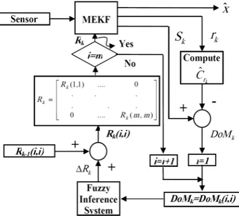
In this case, an on-line fuzzy logic-based adaptive Kalman filter (FL-AKF) is presented [15]-[16] that we proposed and using the fuzzy logic-based adaptive modified extended Kalman filter (FL-AMEKF). The adaptation is in the sense of using a Fuzzy Inference System (FIS) to dynamically adjust the measurement noise covariance matrix Rk from data as they are

obtained. This relaxes the a priori measurement noise statistical assumptions and significantly benefits the extended Kalman filter states estimates if the measurement noise under it operates change or evolves with time. The main advantages derived from the use of a fuzzy technique, with respect to traditional adaptation schemes, are the simplicity of the approach and the possibility of including heuristic knowledge about the phenomenon under consideration. The measurement noise

covariance matrix Rk represents the accuracy of the

measurement instrument, meaning a larger Rk for measured

data implies that we trust this data less and take more account of the prediction. Assuming that the noise covariance matrix Qk is

known, here a FIS based on the technique known as covariance matching [17] has been derived to dynamically adjust the covariance matrix Rk. The basic idea behind the

covariance-matching technique is to make the residuals consistent with their theoretical covariance [12]-[18]. In the FL-AMEKF this is done in three steps: first, having available the innovation sequence or residual rk its theoretical covariance

is calculated as,

k T k k k

k

H

P

H

R

S

=

−

+

(18) in the Kalman filter algorithm. Second, the actual covariance

k r

Cˆ of rk is approximated through averaging inside a moving

estimation window [18] of size M,

∑

=

=

k

i i

T i i

r

r

r

M

C

k

0

1

ˆ

₍₁₉₎

where io = k - M + 1 is the first sample inside the estimation

window. This means that only the last M samples of rk are used

to estimate its covariance. The window size is chosen empirically to give some statistical smoothing. Third, if it is found that the actual value of the covariance of rk has a

discrepancy with its theoretical value, then a FIS derives adjustments for Rkbased on the knowledge of the size of this

discrepancy. The objective of these adjustments is to correct this mismatch as well as possible. In order to detect the size of the discrepancy between Skand

k r

Cˆ a new variable called the Degree of Matching (DoM) is defined as,

k r k

k

S

C

DoM

₌

₋

ˆ

₍₂₀₎ The main idea of adaptation used by a FIS to dynamically tuning Rk is as follows. It can be noted from (18) that an

increment in Rkwill increment Sk and vice versa. This means

that Rk can be used to vary Skin accordance with the value of

DoMk in order to reduce the discrepancies between Sk and k r

Cˆ . From here three general rules of adaptation are defined as:

1. If DoMk ≅0 (this means Sk, and Cˆr_k match almost

perfectly) then maintain Rk unchanged.

2. If DoMk > 0 (this means Sk, is greater than its actual

value

k r

Cˆ ) then decrease Rk.

3. If DoMk < 0 (this means Skis smaller than its actual

value

k r

Cˆ ) then increase Rk.

Note that the matrices

k r

Cˆ , Sk, Rk and DOMkare all of the

same size, thus the adaptation of the (i,i) element of Rkcan be

made in accordance with the (i,i) element of DoMk; i=1,2, ...,

m; m=size of zk. Thus, a single-input-single- output (SISO) FIS

is used to sequentially generate the tuning or correction factors for the elements in the main diagonal of Rk and this correction is

k k

k

i

i

R

i

i

R

R

(

,

)

=

₋1

(

,

)

+

Δ

(21) where

Δ

R

_kis the tuning factor that is added or subtracted from the element (i,i) of Rk at each instant of time,

Δ

R

_k is the

FIS output and DoMk(i,i) is the FIS input. A graphical

[image:4.595.305.545.86.239.2]

representation of this adjusting process is shown in Fig. 1.

Fig. 1. Graphical Representation of the adjusting process of Rk

Following the general rules of adaptation, the FIS can be implemented considering three fuzzy sets for DoMk: N =

Negative, ZE = Zero, and P = Positive; and three fuzzy sets forΔR_k: I = Increase, & M = Maintain, and D = Decrease. These membership functions are shown in Fig. 2. There, the parameters that define the fuzzy sets can be changed in accordance with the system under consideration. Hence, only three fuzzy rules are included in the FIS rule base:

1. If DoMk = N, then

Δ

R

_k = I

2. If DoMk = ZE, then

Δ

R

_k = M

3. If DoMk = P, then

Δ

R

_k = D.

Thus, using the compositional rule of inference sum-prod and the center of area (COA) defuzzification method, Rk is

adjusted in each FL-AMEKF as given in (21). From experimentation it was found that a good size for the moving window in (19) is M =30.

-10 -8 -6 -4 -2 0 2 4 6 8 10 0

0.5

N

Z E

P

(a)

-0.5 -0.4 -0.3 -0.2 -0.1 0 0.1 0.2 0.3 0.4 0.5 0

0.5 1

L

M

I

(b)

Fig. 2. Membership function for a) DoMk b)ΔR_k

III. CSTRPLANT DESCRIPTION

[image:4.595.49.283.166.377.2]

An irreversible and exothermic reaction

A

→

B

takes place inside the jacket CSTR that is shown in Fig. 3 [19]. The reaction is operated by two PI controllers that are used to regulate the outlet temperature and the tank level. A cooling jacket surrounds the reactor and the coolant is water in this case. Negligible heat losses, constant densities, perfect mixing inside the tank and uniform temperature in the jacket are assumed.

Fig. 3. Continuous stirred tank reactor

The equations describing the system are [20]:

o i

F

F

dt

dV

−

=

(22)

Ca RT E k

V Ca F Ca F dt VCa

d a

o i

i ⎟⎟

⎠ ⎞ ⎜⎜

⎝ ⎛

⎟ ⎠ ⎞ ⎜ ⎝ ⎛ −

−

= exp

) (

0 (23)

) (

)

( _{c FT FT}

dt VT d

c_p =

ρ

_{p i i}− _o

ρ

)

(

exp

a 0 j

o

Ca

Ua

T

T

RT

E

k

HV

_⎟⎟

−

−

⎠

⎞

⎜⎜

⎝

⎛

⎟

⎠

⎞

⎜

⎝

⎛

Δ

−

(24)

)

(

)

(

c j 0 j

j j j j j j

j

c

F

T

T

Ua

T

T

dt

dT

c

V

=

ρ

−

+

−

ρ

(25)

[image:4.595.317.525.420.535.2]

research study.

Table I: List of Fault Studied Fault

Fault Name

#1p High inlet feed of reactant Fi+ΔFi

#1n Low inlet feed of reactant Fi−ΔFi

#2p High inlet concentration of reactant Cai+ΔCai

#2n Low inlet concentration of reactant Cai−ΔCai

#3p High inlet temperature of reactant Ti+ΔTi

#3n Low inlet temperature of reactant Ti−ΔTi

#4p High inlet temperature of coolant Tc+ΔTc

#4n Low inlet temperature of coolant Tc−ΔTc

IV. SIMULATION STUDY

In classical control, non-manipulated variables dk are treated

as known inputs with distinct entry in the system state-space model. This distinction between state and non-manipulated variables, however, is not justified from the monitoring perspective using the Kalman filter estimation procedure. Therefore, a new augmented state variable vector

] , [

*

k k k d x

x = is developed by considering the

non-manipulated variables as state variables. To implement this view, the non-manipulated inputs are assumed to be states without dynamics but governed by the following stochastic auto-regressive model equation [21]:

1

1 −

−

+

≈

_{k k}

k

d

w

d

(26) This assumption changes the linearized model formulation, described by Ak, Bk and Hk matrices, to the following

augmented state-space model:

* 1 1 * *

1 * *

− − −

+

=

_{k k k}

k

A

x

B

u

w

x

(27)

* 1 * * *

−

+

=

_{k k}

k

H

x

v

y

(28) Where matrix Bk has been dropped and the new transition

state matrix is defined as follows:

⎥

⎦

⎤

⎢

⎣

⎡

=

×_× ×_×

x x u x

x u u u

n n n n

n n n n

A

B

I

A

*

0

(29) Where nxand nudenote the dimensions of the state (xk) and

[image:5.595.307.549.230.641.2]

manipulated variables (uk), respectively.

Fig. 4 shows the schematic block diagram of the proposed fault detection system used in this simulation study.

Fig. 4. Block diagram for detection and diagnosis with using Fig. 1 and MSDF

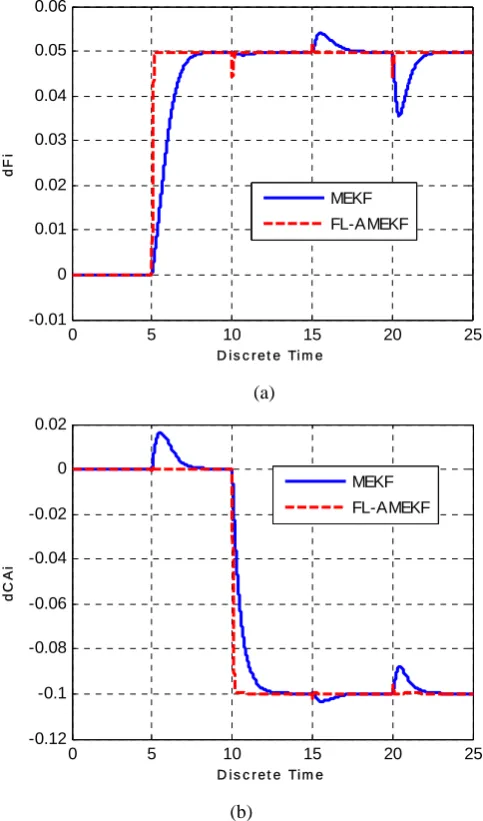
Fig. 5 (a,b,c,d) illustrate the performance results of the process fault detection system for both the MEKF and the

FL-AMEKF algorithms. These figures show the overall result for simultaneous occurrences of fault #1p (ΔFi=5%) at t=5, fault #2n (ΔCai=10%) at t=10, fault #3n (ΔTi=10%) at t=15, fault #4p (ΔTc=5%) at t=20, in the CSTR plant.

We for see performance this methods to process faults diagnosis, selection of faults occurring at different times with different magnitudes. In the other hand, we selected faults in way of that at t=5 we have one fault (fault #1p) and t=10 two faults including fault #1p and fault #2n and t=15 there faults including fault #1p , fault #2n and fault #3n and t=20 each four faults.

0 5 10 15 20 25

-0.01 0 0.01 0.02 0.03 0.04 0.05 0.06

D i s c r e t e Ti m e

dF

i

MEKF FL-AMEKF

(a)

0 5 10 15 20 25

-0.12 -0.1 -0.08 -0.06 -0.04 -0.02 0 0.02

D i s c r e t e Ti m e

dC

Ai

MEKF FL-AMEKF

(b)

Fig. 5(a) shows estimation of fault#1p (high inlet feed of reactant) using MEKF and FL-AMEKF methods. It can be seen from the figure that the estimation using FL-AMEKF method has better performance as the other faults have much less effect on the estimation of fault#1p. The MEKF method has some drawbacks such as:

[image:5.595.47.287.630.689.2]

steady state value.

• The convergence of the estimation is with a greater time constant leading to transient errors.

Fig. 5(b,c,d) showing the same results for faults #2n, #3n, #4p.

0 5 10 15 20 25

-0.1 -0.08 -0.06 -0.04 -0.02 0 0.02

D i s c r e t e Ti m e

dT

i

MEKF FL-AMEKF

(c)

0 5 10 15 20 25

-0.01 0 0.01 0.02 0.03 0.04 0.05 0.06

D i s c r e t e Ti m e

dT

c

MEKF FL-AMEKF

[image:6.595.47.293.140.560.2]

(d)

Fig. 5. Estimation of faults occurring at different times with different magnitudes. (a) dFi fault estimation (b) dCAi fault estimation (c) dTi fault estimation (d) dTc fault estimation.

V. CONCLUSIONS

This research work investigates the usefulness of the MSDF technique to enhance the process fault detection and diagnosis based on the EKF estimation approach. Also, investigates the usefulness of the fuzzy logic to enhance the process fault detection based on the MEKF estimation approach. In real application, however, the exact values of estimation covariances Q and R are not known a priori and hence their time evolutions are usually neglected. This leads to unaccuracy in estimation which can diverge the Kalman filter operation.

An efficient discrete-time MEKF implementation has been presented in this paper to enhance the robustness of the algorithm by preserving both the symmetry and positive definiteness of the state covariance matrix p.

The proposed approach has been tested on a simulation CSTR plant for multiple possible faults occurring at different times. The simulation results demonstrate the superiority of the proposed FL-AMEKF technique in abrupt detection of the occurred faults compared with the classical MEKF approach.

REFERENCES

[1] W. S. Lee, D. 1. Grosh, F. A. Tillman, C. H. Lie, “ Fault Tree analysis, methods and applications: A review”, IEEE Trans. Reliability, Vol.R-34, 1985, pp.194-302.

[2] M. A. Kramer, Jr. B. L. Palowitch, “A Rule Based Approach to Fault Diagnosis Using the Signed Directed Graph”, AIChE Journal,Vol.33, NO.7, 1987, pp.1067-1078.

[3] P. Vaija, I. Turunen, M. Jarvelainen, M. Dohnal, “Fuzzy strategy for failure detection and safety control of complex processes”,

Microelectronics Reliability, Vol. 25,No. 2, 1985, pp. 369-81.

[4] V. Venkatasubramanian, K. Chan, “A Neural Network Methodology for Process Fault Diagnosis”, AIChE Journal, Vol. 35, NO. 12, 1989, pp. 1993-2002.

[5] R. Fickelsherer, D. E. Lamb, P. Dhujati, D. L. Chester, “ Role of Dynamic Simulation in Developing an Expert System for Chemical Process Fault Detection”, Proc. Computer Simulation conf. Society for Computer Simulation, 1986.

[6] R. Isermann, “ Process fault detection based on modeling and estimation methods, A Survey”, Automatica, 1984, pp. 387-404.

[7] D. M. Himmelblau, “Fault Detection and Diagnosis in Chemical and Petrochemical Processes”, Amsterdam- Elsevier, 1978.

[8] A. S. Willsky, “A survey of design methods for failure detection systems”, Automatica, 1976, pp. 601-611.

[9] M., S. Grewal & A. P. Andrews, “Kalman Filtering Theory and Practice Using MATLAB (Second ed.)”. New York, NY USA: John Wiley & Sons, Inc, 2001.

[10] G. Welch, G. Bishop, An Introduction to the Kalman Filter, University of North Carolina at Chapel Hill, Department of Computer Science, Chapel Hill, 2001.

[11] P. S . Maybeck, “Stochastic Models, Estimation and Control”, New York

Academic, Vols. I and II, 1982.

[12] R. K. Mehra, “On the identification of variances and adoptive Kalman filtering”, IEEE Trans. Automatic Control. Vol. AC-15, No. 2, 1970, pp. 175- 184.

[13] R. J. Fitzgerald, “Divergence of the Kalman filter”, IEEE Trans.

Automatic Control, Vol. AC-16. No. 6, 1971, pp. 736- 747.

[14] S. Sangsuk-lam. and T. Bullock, “Analysis of discrete-time Kalman filtering under incorrect noise covariances”, IEEE Trans, On Automatic Control, Vol. 35, No. 12, Dec. 1990, pp. 1304-1308.

[15] P. J. Escamilla-Amhrosio and N. Mort, “Development of a fuzzy logic-based adoptive Kalman filter”, proceeding of the 2001 European

Control Conference. Porto. Portugal, Sep. 2001, pp. 1768-1773. [16] P. J. Escamilla-Ambrosio and N. Mort, “Multi-sensor Data Fusion

Architecture Based on Adaptive Kalman Filters and Fuzzy Logic Performance Assessment”, Department of Automatic Control and

Systems Engineering, University of Sheffield, Sheffield, UK, ISIF 2002, pp. 1542-1549.

[17] R. K, Mehra, “Approaches to adaptive fi1ltering”, IEEE Trans.

Automatic Control. Vol. AC-17, Oct. 1972, pp. 693- 698,.

[18] A. H. Mahamed, and K. P. Shwm, “Adoptive kalman filtering for INS/GPS”, Journal of Geodesy. Vol. 73, No. 4, 1999, pp. 193-203. [19] N. Sawattanakit, V. Jaovisidha, “Process Fault Detection and Diagnosis in

CSTR System Using On-line Approximator”, IEEE, 1998, pp. 747-750. [20] W. L. Luyben, “Process Modeling Simulation and Control for Chemical

Engineers”, McGraw-Hill, 2nd edition, 1989.

[21] E. Musulin, C. Benqlilou, M. J. Bagajewicz, L. Puigjaner, “Instrumentation design based on optimal Kalman filtering”, Journal of

[image:6.595.290.549.213.758.2]