Munich Personal RePEc Archive
Maximum likelihood estimation and
inference for high dimensional nonlinear
factor models with application to
factor-augmented regressions
Wang, Fa
Cass Business School, City, University of London
18 May 2017
Online at
https://mpra.ub.uni-muenchen.de/93484/
Maximum Likelihood Estimation and Inference for
High Dimensional Nonlinear Factor Models with
Application to Factor-augmented Regressions
Fa Wang
yMay 19, 2019
Abstract
This paper reestablishes the main results in Bai (2003) and Bai and Ng (2006) for nonlinear factor models, with slightly stronger conditions on the relative magnitude of N(number of subjects) and T(number of time periods). Convergence rates of the estimated factor space and loading space and asymp-totic normality of the estimated factors and loadings are established under mild conditions that allow for linear models, Logit, Probit, Tobit, Poisson and some other nonlinear models. The probability density/mass function is allowed to vary across subjects and time, thus mixed models are also allowed for. For factor-augmented regressions, this paper establishes the limit distributions of the parameter estimates, the conditional mean, and the forecast when factors estimated from nonlinear/mixed data are used as proxies for the true factors.
Keywords: Factor model, Mixed measurement, Maximum likelihood, High dimension, Factor-augmented regression, Forecasting
JEL Classi…cation: C13, C35
We would like to thank the editor Jianqing Fan, the associate editor and two referees for their valuable comments and suggestions. We would also like to thank Jushan Bai, Mingli Chen, Xiaohong Chen, Ivan Fernandez-Val, Kunpeng Li, Giovanni Urga, Martin Weidner and seminar participants at Chinese University of Hong Kong, Cass Business School, University of Connecticut and 2017 Asian Meeting of Econometric Society for helpful comments and suggestions.
1
Introduction
High dimensional factor models where a large number of time series are simultaneously driven by a small number of latent factors provide a powerful framework to analyze high dimensional data. Accompanied by an ever-increasing data size, the literature for this model recently experienced a wave of development. For example, Bai and Ng (2002) and Bai (2003) respectively show that utilizing the high dimensionality, we are able to consistently determine the number of factors and establish the asymptotic normality of the estimated factors and loadings. High dimensional factor models have also been successfully used in macroeconomic monitoring and forecasting, business cycle analysis, asset pricing, risk measurement, see for example Stock and Watson (2002, 2016), Bernanke, Boivin and Eliasz (2005), Ross (1976) and Campbell, Lo and Mackinlay (1997), to name a few.
So far the literature only considers linear factor models. However, in many macro-economic or …nancial applications and in most micromacro-economic applications, the rela-tionship between the dependent variable and the factors could be nonlinear. Repre-sentative examples include but not limited to the case where the dependent variable is categorical. Direct extension of existing theory, e.g., Bai (2003) and Bai and Li (2012, 2016), to categorical data is not feasible because essentially both methods are based on the covariance matrix of the continuously distributed dependent variable. This paper seeks to establish a new estimation and inferential theory for high dimen-sional nonlinear factor models. More speci…cally, this paper considers the following single-index factor model: For i= 1; :::; N and t= 1; :::; T,
xit git( 0it): (1)
xitis the observed data for thei-th subject at timet. git( j )is some known probability
(density or mass) function of xit allowed to vary across i and t. Note that git( j ) is
the conditional probability function. Weak cross-sectional and serial dependence of
xit is allowed. 0it = ft00 i0, and ft0 and 0i is an r dimensional vector of factors and
studied in a separate paper.
For engineering, this model has been successfully used in data compression, visu-alization, pattern recognition and machine learning. For social sciences, this model also plays important role in psychology and education. For economics and …nance, possible applications are partially listed below:
(1) Macroeconomic forecasting, factor-augmented vector autoregression and busi-ness cycle analysis: In these areas, common factors are predominantly estimated by principal components using continuous data, see Stock and Watson (2002), Bernanke, Boivin and Eliasz (2005) and Bai and Ng (2006). Little attention has been paid to the treatment of categorical or mixed measurement data even though many data sets are of this type. For example, letx1t be the GDP, x2t be the consumer con…dence index
(categorical), x3t be the interest rate announcement of FOMC, etc, at time t. Let
f0
t denote some macroeconomic factors, then xit is nonlinearly linked to 0it = ft00 0i
through some known link function. While mixed measurement data are quite infor-mative, they cannot be directly handled by principal components estimation. This paper provides a rigorous solution to this issue.
(2) Credit risk analysis: Default correlation modelling has direct implications for CDO (collateralized debt obligations) pricing, bond portfolio management and commercial bank risk management. Intuitively, default correlation originates from common exposures to business cycle, monetary policy, market sentiment and other …nancial or sector factors. Factor models provide a parsimonious way for analyzing default correlation and underlies many risk models used in practice. In a representa-tive case, 0
it+eit is the value of company i at time t, eit is the idiosyncratic error
term,f0
t is the common factors andxit is nonlinearly linked to 0it. xitcould be rating
category companyibelongs to, or the binary variable describing the default event, or the credit spread of its bond, or its stock return, or its stock volatility at timet. For more details on default correlation modelling and estimation, see Schonbucher (2000), McNeil and Wendin (2007), Koopman and Lucas (2008), Koopman, Lucas and Mon-teiro (2008), Koopman, Lucas and Schwaab (2011), Creal, Schwaab, Koopman and Lucas (2014) and the references therein.
eco-nomics, welfare economics and economics of education, researchers frequently en-counter the problem of measuring the socio-economic status (more speci…cally the wealth or consumption) of a household or an individual. A good measure, serving as either the explanatory or the dependent variable, is crucial for these studies. Direct accurate measures of household wealth or consumption usually are not available or not reliable. Instead, the survey data contains many reliable yet categorically distrib-uted proxies, such as living conditions and ownership of durables or assets. Treating these proxies as the dependent variables and household wealth as the latent explana-tory factor, household wealth could be estimated from the data of these proxies. For example, let xit be the i-th proxy of householdt and let ft0 be the wealth of
house-holdt, thenxit is nonlinearly linked to 0it=ft00 0i through some known link function
implied by economic theory. Filmer and Pritchett (2001) follows this approach to construct wealth index for estimating the e¤ect of wealth on educational enrollments in India. The Filmer-Pritchett procedure simply extracts the factor from the binary proxies directly by principal component. Rigorously speaking, this procedure is lack of theoretical support and may lead to misleading results.
For all the above and future applications, it is in urgent need to develop a theoret-ically justi…ed method for estimating the factors and loadings from high dimensional nonlinear/mixed data. It is also necessary to establish the asymptotic properties of the proposed estimator under the high dimensional setup. Such asymptotic prop-erties are needed to characterize the conditions under which the estimation error is negligible when estimated factors are used as regressors and to construct con…dence intervals when estimated factors represent economic indices.
Bai (2003) is a special case of this paper. The probability function is also allowed to vary across i and t, thus a mixture of these models is allowed for. This paper also establishes the limit distributions of the parameter estimates, the conditional mean as well as the forecast for factor-augmented regression models when the estimated factors are used as proxies for the true factors. This result generalizes Bai and Ng (2006) to allow us using factors extracted from nonlinear/mixed data.
In the statistics literature, classic factor analysis has been successfully extended to categorical data and mixed data, see for example, Bartholomew (1980), Moustaki (1996), Bartholomew and Knott (1999), Moustaki (2000), Moustaki and Knott (2000) and Joreskog and Moustaki (2001), to name a few. All these papers assume N
is …xed and much smaller than T. While factors are typically of primary interest in economic applications, factors can not be consistently estimated under the …xed
N large T setup. This limitation and the urgent need to handle high dimensional mixed data recently has motivated researchers to explore possible solution. Ng (2015) reviews alternative methods of constructing factors that can potentially be extended to categorical data and explores their numerical properties.
This paper provides a general theory for factor analysis of high dimensional non-linear data. Since factors and loadings are treated as parameters to be estimated, the number of parameters tend to in…nity as N and T tends to in…nity jointly. This paper solves this problem by utilizing the fact that for factor model, the Hessian is as-ymptotically block diagonal and the tensor of third order derivatives is sparse. More speci…cally, elements in the diagonal blocks of the Hessian are Op(N)or Op(T)while elements in the o¤-diagonal blocks are Op(1). This paper shows that under relevant regularity conditions, the presence of these nonzero o¤-diagonal blocks has no e¤ect on the asymptotic properties of the estimated factors and loadings. Asymptotic block diagonality of the Hessian also provides explanation for Bai (2003)’s results from the perspective of extremum estimation.
diag-onality comes from arti…cial reparametrization. More recently, Fernandez-Val and Weidner (2016) and Chen, Fernandez-Val and Weidner (2014, 2018) utilize asymp-totic diagonality of the incidental parameter Hessian to derive the limit distributions of the regression coe¢cients and the average partial e¤ects in nonlinear panel mod-els. For the estimated factors and loadings, Chen et al. (2014, 2018) establishes the average consistency, while this paper also establishes the convergence rates, the limit distributions and the e¤ect of using estimated factors in factor-augmented regression. The rest of the paper is organized as follows. Section 2 introduces notations and preliminaries. Section 3 discusses the assumptions. Section 4 presents the limit theory. Section 5 presents results for factor-augmented regressions. Section 6 introduces computation algorithms. Section 7 presents simulation results. Section 8 concludes. All proofs are relegated to the appendix.
2
Notations and Preliminaries
The log-likelihood1 function is
L(Xjf; ) =XN i=1
XT t=1lit(f
0
t i); (2)
where lit( it) = loggit(xitj it) and it = ft i0 , X is the T N matrix of observed
data and xit is the element on the t-th row and the i-th column, f = (f10; :::; fT0)0 a
T r dimensional vector and = ( 01; :::; 0N)0 is a N r dimensional vector. git( j ) is
allowed to vary across i and t, thus data following di¤erent models (e.g., discretely and continuously distributed time series) can be merged directly to extract common factors. We consider the following representative examples.
Example 1 (Linear): lit(f0
t i) = 12(xit ft i0 )2.
Example 2 (Probit): lit(f0
t i) = xitlog (ft i0 ) + (1 xit) log(1 (ft i0 )), where ( ) is the CDF of the standard normal distribution.
1Whenx
Example 3 (Logit): lit(ft i0 ) =xitlog (ft i0 ) + (1 xit) log(1 (ft i0 )), where ( )
is the CDF of the logistic distribution.
Example 4 (Tobit): Suppose xit = xit if xit > 0 and xit = 0 if xit 0, where
xit = f0
t i+eit and eit is N(0;1). The likelihood function is lit(ft i0 ) = 12(xit
f0
t i)21(xit >0) + log(1 (ft i0 ))1(xit= 0), where 1( ) is the indicator function.
Example 5 (Poisson): lit(ft i0 ) = ef
0
t i + kf0
t i logk!, because P(xit = k) =
p(k; ) = e k=k! and =ef0
t i.
Let = ( 0; f0)0,F = (f
1; :::; fT)0, = ( 1; :::; N)0. Similarly, for the true values of
the factors and the loadings, letf0 = (f00
1 ; :::; fT00)0, 0 = ( 001; :::; 00N)0, 0 = ( 00; f00)0,
F0 = (f0
1; :::; fT0)0 and 0 = ( 01; :::; 0N)0. Also, let @ lit( it), @ 2lit( it) and @ 3lit( it)
be the …rst, second and third order derivative of lit( ) evaluated at it, respectively.
When these derivatives are evaluated at 0
it, we suppress the argument and simply
write @ lit, @ 2lit and @ 3lit.
Both factors and loadings are treated as parameters. Note that for anyF, and anyr r invertible matrix G,F G and (G0) 1 has the same likelihood asF and .
To uniquely …xF and , we impose the normalization such that (1)F0F is diagonal,
(2) 0 is diagonal, (3) 1
TF
0F = 1
N
0 , i.e., the estimated factors and loadings are the
solution of maximizingL(Xjf; )under constraints (1)-(3). As explained in Remark 1 below, the solution of this constraint maximization problem is always the same as the solution of maximizing Q(f; ) = L(Xjf; )+P(f; ), where
P(f; ) = c 8N T
Xr p=1(
1
N XN
i=1 2
ip 1
T XT
t=1f 2
tp)2
c
2
T N
Xr p=1
Xr q=p+1(
XN
i=1 ip iq) 2
c
2
N T
Xr p=1
Xr q=p+1(
XT
t=1ftpftq)
2; (3)
is a penalty function,0< c < bLand bL is lower bound ofj@ 2lit( it)j as presented in
normalization (1)-(3) is slightly di¤erent from the classical normalization 1
TF
0F =I
r
and 0 being diagonal. We choose this normalization because with penalty (3), the
Hessian matrix of Q(f; )has some convenient structure for analyzing its asymptotic behavior. If we choose another normalization, all results of this paper still hold, except for a di¤erent rotation matrix2.
Let B(D) denote the neighborhood kfk1 D and k k1 D for some large
D > 0, and let f^= ( ^f0
1; :::;f^T0)0 and ^ = (^
0 1; :::;^
0
N)0 be the solution of maximizing
Q(f; ) within B(D). We will explain why taking f^and ^ within B(D) in Remark 2 below. Let ^it = ^f0
t^i, ^ = (^
0
;f^0)0, F^ = ( ^f
1; :::;f^T)0 and ^ = (^1; :::;^N)0. The r
columns ofF^ are ordered according to their Euclidean norm, from the largest to the smallest. Ther columns of ^ are ordered in the same way.
Throughout the paper, let (N; T)! 1 denote N and T going to in…nity jointly,
N T = minfN
1 2; T
1 2g,D
N T =
"
N IN r 0 0 T IT r
#
, DT N =
"
T IN r 0 0 N IT r
#
.
d
!denotes convergence in distribution. "w.p.a.1" denotes "with probability approach-ing 1". For matrixA, let min(A)denote its smallest eigenvalue andkAk,kAkF,kAk1,
kAk1 and kAkmax denote its spectral norm, Frobenius norm, 1-norm, in…nity norm
and max norm respectively. When A has N r rows, divide A into N blocks with each block containing r rows and let [A]iq denote the q-th row in the i-th block and [A]i = ([A]0
i1; :::;[A]0ir)0 denote the i-th block.
Remark 1 First note that for anyF and , there exists a unique matrixG such that
P(F G; (G0) 1) = 0, and P(F G; (G0) 1) < 0 for other G. If F and maximizes
Q(F; ), then P(F; ) = 0 because otherwiseP(F; )<0 and we can …nd the appro-priateG such thatL(XjF; ) = L(XjF G; (G0) 1)and P(F G; (G0) 1) = 0, which
implies Q(F; ) < Q(F G; (G0) 1), a contradiction. Thus the solution of
maximiz-ing Q(F; ) is the same as the solution of maximizing Q(F; ) under the constraints
P(F; ) = 0. The latter is the same as the solution of maximizing L(XjF; ) un-der the constraints P(F; ) = 0, which is the same as the solution of maximizing
L(XjF; ) under the constraints (1)-(3).
2To show this, we …rst prove the results for this normalization, and then prove the results still
3
Assumptions
Assumption 1 (i) T 1F00F0 !p
F for some positive de…nite F. There exists
M >0 such thatkf0
tk M for all t.
(ii) N 1 00 0 !p for some positive de…nite . There exists M > 0 such that 0
i M for all i.
Assumption 2 (i) lit( )is three times di¤erentiable.
(ii) There exists bU > bL > 0 such that bL @ 2lit( it) bU within a compact space of it.
(iii) j@ 3lit( it)j bU within a compact space of it.
Assumption 3 There exists M > 0 such that for allN and T: (i) E(j@ litj ) M for some >14 and all i and t.
(ii) T 1PT s=1
PT
t=1( N(s; t))2 M, where N(s; t) = N 1
PN
i=1E(@ lis@ lit).
(iii) For every (t; s), E(N 12 PN
i=1[@ lis@ lit E(@ lis@ lit)])2 M.
Assumption 4 There exists M > 0 such that for some >2 and for all N and T,
E(N 1PN i=1 T
1 2 PT
t=1@ litft0 ) M,
E(T 1PT t=1 N
1 2 PN
i=1@ lit 0
i ) M.
Assumption 5 (i) E N 12T 1 2 PN
i=1
PT t=1(T 1
PT
t=1@ 2litft0ft00) 1ft0@ lit@ lis
2
M for any s and
E N 12T 1 2 PN
i=1
PT
t=1(N 1
PN
i=1@ 2lit 0
i 00i ) 1 0i@ lit@ ljt
2
M for any j.
(ii) E N 12T 1 2 PN
i=1
PT t=1(T 1
PT
t=1@ 2litft0ft00) 1@ litft0 00i
2
M and
E N 12T 1 2 PN
i=1
PT
t=1(N 1
PN
i=1@ 2lit 0
i 00i ) 1@ lit 0ift00
2
M.
E N 12T 1 2 PN
i=1
PT t=1(T 1
PT
t=1@ 2litft0ft00) 1@ litft0 00i @ 2lis
2
M for any s
and
E N 12T 1 2 PN
i=1
PT
t=1(N 1
PN
i=1@ 2lit 0
i 00i ) 1@ lit 0ift00@ 2ljt
2
M for any j.
(iii) for any i, T 1PT
t=1@ 2litf0
tft00 p
! iF and T
1 2 PT
t=1@ litft0 d
! N(0; iF)
(iv) for any t, N 1PN
i=1@ 2lit 0
i 00i ! t and N
1 2 PN
i=1@ lit 0
i d
! N(0; t )
for some positive de…nite t and t .
Assumption 6 The eigenvalues of the r r matrix ( F ) are di¤erent.
Assumption 7 N
3
T
3
(N+T)
1
N T !0 as (N; T)! 1.
Assumption 1(i) corresponds to Assumption A in Bai (2003). Factors are allowed to be dynamic with arbitrary dynamics. Assumption 1(ii) is exactly the same as As-sumption B in Bai (2003), and ensures each factor has a nontrivial contribution. Note that here kf0
tk and 0i are assumed to be uniformly bounded. This assumption is
the same as Bai and Li (2016), but stronger than Bai (2003), which only assumes uniform boundedness of Ekf0
tk
4
and E 0i
4
. In general, compactness of parameter space is quite common for nonlinear models, e.g., Newey and McFadden (1994), Jen-nrich (1969) and Wu (1981). Under the current setup, this assumption is necessary because the convergence rate (and hence limit distribution) of f^t is not uniform over
the parameter space off0
t if @ 2lit(f00
t 0i) !0askft0k ! 1. In other words, in such
cases the convergence rates off^t will not be the same3 for all t.
Assumption 2(i) imposes smoothness condition on the log-likelihood function. As-sumption 2(ii) and (iii) assumes that the log-likelihood function is concave, the second order derivatives are bounded below and above, and the third order derivatives are bounded above. The boundedness of the second and third order derivatives is needed to control the remainder term in the expansion of the …rst order condition4. The
boundedness from below of the second order derivatives together with boundedness of it are used to show consistency of the estimated factors and loadings. We
ver-ify in Appendix D that Logit, Probit, Poisson and Tobit all satisfy Assumption 2.
3For example, consider the case f0
t is one dimensional and @ 2lit(ft00
0
i) converges to zero
monotonically as f0
t ! 1. Let t = arg maxft and t = arg minft. Then convergence rate of
^
ft would be slower thanf^t as(N; T)! 1.
4Newey and McFadden (1994) only requires two times continuously di¤erentiable because it
These are most frequently used nonlinear models. For other models, readers can check accordingly.
Assumptions 3-5 are generalization of Assumptions C, D and F in Bai (2003) in the nonlinear setup. When the model is linear,@ lit is the error term "eit" and@ 2lit
is a constant, and Assumptions 3-5 reduce to Assumptions C, D and F in Bai (2003) respectively (with slight modi…cation on the value of and and the statement of Assumption F1). As Bai (2003), distribution of xit is allowed to be heterogeneous
over i and t, and limited cross-sectional and serial dependence of xit is also allowed.
Ifxit is independent overi andt conditional on the factors and loadings, Assumption
3(ii) and (iii), Assumption 4 and Assumption 5 can be easily veri…ed. If there is no conditional independence, these assumptions still can be veri…ed provided certain weak dependence conditions are imposed on. We follow Bai (2003)’s treatment in presenting Assumptions 3-5.
Assumption 6 is a crucial identi…cation condition and is the same as Assumption G in Bai (2003). It guarantees that there exists uniqueF and such thatF 0 =F0 00,
F0F and 0 are diagonl and F0F=T = 0 =N. Assumption 7 is quite weak if and
are large. Note that except for some well-designed mathematical counterexamples, Assumptions 3(i) and 5 indeed hold with very large and .
4
Limit Theory for Estimated Factors and
Load-ings
For anyF0and 0, let 2
1 > ::: > 2rbe the eigenvalues ofN 1T 1( 00 0)
1
2F00F0( 00 0) 1 2
and be the matrix of corresponding eigenvectors, and let V =diag( 2
1; :::; 2r).
As-sumption 1 implies that V converges in probability to the diagonal matrix of eigen-values of
1 2
F
1
2 and converges in probability to the matrix of eigenvectors of 1
2
F
1
2. Let G = ( 00 0
N )
1
2 V
1
4, G converges in probability to a constant matrix.
Assumption 6 guarantees G is unique for N and T large enough. Relationship of
FG=F0G and G = 0(G 1)0. It can be easily veri…ed that FG G0 =F0 00 and
1
TF
G0FG = 1
N
G0 G =V1
2: (4)
Similar to the notation in Section 2, let FG = (fG
1 ; :::; fTG)0, G = ( G1; :::; GN)0,
fG = (fG0
1 ; :::; fTG0)0, G
= ( G10; :::; GN0)0 and G
= ( G0; fG0)0. By de…nition of FG, it
is easy to see that fG
t = G0ft0 and iG = G 1 0i. We consider G because G is the
unique rotation such that P( G; fG) = 0.
Let S( ) = @ Q( ), S ( ) = @ Q( ) and Sf( ) = @fQ( ) denote the score, it
follows that S( ) = (S0( ); S0
f( ))0. Let H( ) = @ 0Q( ) be the Hessian matrix.
Decomposition ofH( )and the expression of each component is presented in Appen-dix A. We suppress the argument whenS( )andH( )are evaluated at G, i.e.,S=
S( G)and H= H( G).
Remark 2 B(D) is designed such that (1) f^0
t^i is uniformly bounded over i and t,
(2) G lies in5 B(D
2) w.p.a.1. Fact (1) is crucial for proving average consistency of
^, see Proposition 1 below. Fact (2) guarantees that G lies in the interior of B(
D).
4.1
Consistency
There are two di¢culties in establishing consistency. First, the number of parameters tends to in…nity jointly with N and T. Thus the classical procedure for extremum estimators, e.g., Newey and McFadden (1994), is no longer applicable. Second, the parameters are present in both dimensions and the likelihood function is nonconcave with respect to the parameters. Thus it is not feasible to extend the proof strategy of large dimensional nonlinear panels to the current setup, because they either require there is only individual e¤ects or time e¤ects (see for example, Hahn and Newey (2004) and Hahn and Kuersteiner (2011)), or require global concavity of the likelihood function (Fernandez-Val and Weidner (2016)). Inspired by Lemma 1 of Chen et al. (2014), this paper solves the di¢culties by utilizing the boundedness from below of
@ 2lit( it) over the compact parameter space.
5Note that fG
1 and
G
1 are bounded w.p.a.1, becausef
0
t and
0
i are uniformly bounded
andkGk is bounded w.p.a.1. Thus G lies inB(D
Proposition 1 (Average Consistency) Under Assumptions 1-3 and 6, as(N; T)!
1, f^ fG =O p(
q
T
N T) and
^ G =O p(
q
N
N T).
A remaining issue is that S(^)is not necessarily zero, because the criterion func-tion is not globally concave. If S(^) 6= 0, then we can not utilize the …rst order conditions to move forward. We next show that S(^) = 0 w.p.a.1. First, Propo-sition 1 implies that ^ lies in the neighborhood D
1 2
N T(
G) m w.p.a.1. By
de…nition, ^ maximizes the likelihood withinB(D). Thus ^ maximizes the likelihood within B(D)\ D
1 2
N T( G) m w.p.a.1. Second, we show in the Appendix that
within the regionB(D)\ D
1 2
N T( G) m, w.p.a.1, the criterion function is
con-cave (see Lemma 3) and there exists a zero point of S( ). This implies that the zero point should maximize the likelihood within B(D)\ D
1 2
N T(
G
) m w.p.a.1. Thus ^ must be the zero point w.p.a.1.
Proposition 2 Under Assumptions 1-4, 6 and 7, S(^) = 0 w.p.a.1.
All subsequent results do not rely on Assumption 7 directly. They rely on As-sumption 7 purely because they rely on Proposition 2. Bai and Ng (2002) and Bai (2003) do not need any condition on the relative magnitude of N and T because in the linear setup the principal component estimator is just the global maximum, i.e., Bai and Ng (2002) and Bai (2003) do not have the di¢culty6 we encounter here.
An intermediate step for Proposition 2 is the following uniform rates.
Proposition 3 (Uniform Consistency) Under Assumptions 1-4 and 6,
(i) ^ G
1 =Op(
N
2
T
2
(N+T)
1
T12 ), (ii)
^
f fG
1 =Op(
N
3
T
3
(N+T)
1
N12 ).
Note that normally and could be large, and in such case ^ G
1 and
^
f fG
1 is approximately Op(T
1
2) and Op(N 1
2), respectively. Thus these rates
are more accurate than Bai (2003)’s Proposition 2 when and are large.
4.2
Convergence Rates
Now we can utilize the …rst order conditions S(^) = 0 to move forward. Using the integral form of the mean value theorem for vector-valued functions7 to expand
the …rst order conditions, we have 0 = @ Q(^) = S + ~H (^ G), where H~ =
R1 0 H(
G
+s(^ G))ds R01H(s)ds. It follows that ^ G = H~ 1S and
N 12(^ G)
T 12( ^f fG)
!
=D
1 2
N T(^ G) =N
1 2T
1 2( D
1 2
T NHD~
1 2
T N) 1D
1 2
T NS; (5)
whereDN T andDT N are normalization matrices de…ned in Section 2. Given
Assump-tion 4, it is easy to see that D
1 2
T NS =Op((N+T)
1
2). Utilizing the structure ofH( )
and eigenvalue perturbation technique, we show in the Appendix (Lemma 3) that the largest eigenvalue of( D
1 2
T NH( )D
1 2
T N) 1 isOp(1)uniformly within the neighborhood
B(D)\ D
1 2
N T( G) mfor somem >0. Since^lies inB(D)\ D
1 2
N T( G)
mw.p.a.1, this implies that ( D
1 2
T NHD~
1 2
T N) 1 isOp(1). Thus we have the following
result:
Theorem 1 (Average Rate) Under Assumptions 1-4, 6 and 7, f^ fG =Op(T12 N T)
and ^ G =Op(N12
N T).
Theorem 1 establishes the convergence rate of the estimated factor space and the estimated loading space. In applications where estimated factors are used as proxies for the true factors, e.g., forecasting, portfolio construction, Theorem 1 provides the foundation for characterizing the e¤ect of using estimated factors. In this paper, we shall use Theorem 1 to show the limit distributions of ^i Gi and f^t ftG, and limit
distribution of the parameter estimates in factor-augmented regressions.
Remark 3 The key step for Theorem 1 is to show that ( D
1 2
T NH( )D
1 2
T N) 1 is
Op(1)uniformly within B(D)\ D
1 2
N T(
G
) m. Lemma 5 of Chen et al. (2014)
proves similar result for the case of one factor. To generalize from one factor to
multiple factors, there are some purely mathematical di¢culties. This paper solves
7Note that the standard mean value theorem does not hold for vector-valued functions. For more
the di¢culties in step (2) of Lemma 2 and Lemma 3. Step (1) of Lemma 2 is similar
to (and inspired by) Lemma 5 of Chen et al. (2014).
4.3
Limit Distributions
Now we proceed to to establish the limit distributions of the estimated factors and loadings. First, it is not feasible to extend Bai (2003)’s method of deriving the limit distribution off^t ftG to the nonlinear setup, because Bai (2003)’s method relies on
expression A.1 in Appendix A of Bai (2003), a crucial decomposition identity that does not hold in nonlinear setup. Second, noting that ^i can be regarded as the
maximum likelihood estimator when f^is used for fG and vice versa, another choice
is to expand the …rst order conditions PTt=1@ lit( ^f0
t^i) ^ft= 0 at Gi and use Theorem
1 to study the e¤ect of using f^for fG and ^ for G
. When the model is linear, Bai (2003) uses this method to establish the limit distributions of ^i Gi . However,
as explained in Remark 4 below, this method is not promising when the model is nonlinear.
Remark 4 Using the integral form of the mean value theorem, the expansion of the
…rst order conditions is
0 =XT
t=1@ lit( ^f 0
t Gi ) ^ft+
XT t=1[
Z 1
0
@ 2lit( ^f0
t( Gi +s(^i Gi )))ds] ^ftf^t0(^i Gi ): (6)
The …rst term on the right hand side equals
XT
t=1(@ lit)f
G t +
XT
t=1[@ lit( ^f 0
t Gi ) @ lit]ftG +XT
t=1(@ lit)( ^ft f
G t ) +
XT
t=1[@ lit( ^f 0
t Gi ) @ lit]( ^ft ftG). (7)
When the model is linear, without loss of generality, suppose lit( it) = 1 2(xit
it)2. Then @ 2lit( ) always equals 1 and fG
t , Gi , f^t, ^i, @ lit and @ lit( ^ft0 Gi ) can
be replaced by "H0F0
t", "H 1 0i", "F~t", "~i", "eit" and " ( ~Ft H0Ft0)0H 1 0i +
eit" in Bai (2003) respectively. It follows that the four terms in expression (7)
be-comes "PTt=1H0F0
teit", "
PT
t=1H0Ft0( ~Ft H0Ft0)0H 1 0i", "
PT
t=1( ~Ft H0Ft0)eit" and
term on the right hand side of equation (6) becomes " PTt=1F~tF~t0(~i H 1 0i)" in
Bai (2003). "T 12 PT
t=1H0Ft0eit" is normally distributed in the limit. Lemma B.2,
Lemma B.1 and Lemma A.1 in Bai (2003) shows respectively that the last three terms
of expression (7) are Op( T
2
N T), which is dominated by the …rst term if T 1
2=N ! 0. Lemma B.2 and Lemma A.1 in Bai (2003) also shows that "T 1PT
t=1F~tF~t0" converges
in probability to some constant matrix. These together shows that "T12(~i H 1 0
i)"
is normally distributed in the limit.
When the model is nonlinear, we have already reestablished Lemma A.1 of Bai
(2003) in Theorem 1. It is also feasible to reestablish Lemma B.1 and Lemma B.2 of Bai (2003), as shown in Lemma 11 in the Appendix. The di¢culty is that we can not
get the accurate rate of the magnitude of PTt=1[@ lit( ^ft0 Gi ) @ lit]ftG, because we do
not have an analytical expression for @ lit( ^f0
t Gi ) @ lit.
To solve this problem, we expand the …rst order conditions S(^) = 0 at G.
0 =S(^) =S+H (^ G) + 1 2R;
where R = (R0; R0
f)0. R and Rf is N r and T r dimensional with element R ;iq = (^ G)0@ 0
iqQ( iq)(^
G)andR
f;tq = (^ G)0@ 0f
tqQ( tq)(^
G)respectively. iq and tq are linear combinations of ^ and
G
. Thus
^ G = H 1S 1
2H
1R; (8)
and ^i Gi = [^ G]i = [H 1S]i 1 2[H
1R]i: (9)
Utilizing the structure of H, we show in Appendix C.5 that
[H 1S]i = (XT t=1@
2litfG
t ftG0) 1
XT
t=1@ litf
G
t +Op(N
1 2T
1
2): (10)
does not matter. In current context,H is not block diagonal, but the elements in its diagonal blocks are much larger than the elements in its o¤-diagonal blocks (Op(N
1 2)
or Op(T
1
2) versus Op(1)). Based on this observation and the structure of H, we
show that in the expansion of [H 1S]i, the extra terms resulting from those nonzero
o¤-diagonal blocks together have order Op(N 12T 1 2).
Based on the structure of H, Theorem 1 and Proposition 4 presented below, we show in Appendix C.5 that
[H 1R]i =Op(N
3
T3
2
N T
): (11)
Thus if T
1 2 2 N TN
3
T3 ! 0, k[H 1R]ik would be o
p(T
1
2) and hence dominated by the
…rst term on the right hand side of equation (10).
Proposition 4 (Individual Rate) Under Assumptions 1-4, 6 and 7, ^i Gi =
Op( N T1 ) for each i and f^t ftG =Op( N T1 ) for each t.
Remark 5 The proof of Proposition 4 is based on expression (7) and utilizes
Cauchy-Schwarz inequality and Theorem 1. The rate Op( 1
N T) is not sharp, but enough for calculating the order of [H 1R]i.
Remark 6 The reason that the remainder term [H 1R]i is asymptotically negligible
is because the tensor of third order derivatives is sparse. For example, it’s easy to see
that PNi=1PTt=1@ k jfslit( ) = 0 if k 6=j, and
PN i=1
PT
t=1@ kflfslit( ) = 0 if l6=s.
From equations (10) and (11), and the symmetry between ^i and f^t, we have the
the following theorem.
Theorem 2 (Individual Limit Distribution) Under Assumptions 1-7,
T12(^i G
i ) d
! N(0; G 1 iF1 iF iF1G0 1) if
T12
2
N T
N3T3 ! 0;
N12( ^f
t ftG) d
! N(0; G0 t1 t t1G) if
N12
2
N T
where G=plimG, and iF, iF, t and t are de…ned in Assumption 5.
Asymp-totic variance of ^i and f^t can be estimated by
var = T(XT t=1@
2lit( ^ft0^i) ^ftf^t0) 1(
XT
t=1(@ lit( ^f 0
t^i))2f^tf^t0)(
XT t=1@
2lit( ^ft0^i) ^ftf^t0) 1;
varf = N(
XN i=1@
2lit( ^f0
t^i)^i^
0
i) 1(
XN
i=1(@ lit( ^f 0
t^i))2^i^
0
i)(
XN i=1@
2lit( ^f0
t^i)^i^
0
i) 1:
Theorem 2 not only allows discrete dependent variables but also allows the prob-ability function to di¤er across individuals and time. The huge amount of discrete data in macroeconomic and …nancial studies thus can be utilized, either by them-selves or merged with continuous data, to extract information on common shocks or the state of the economy or other relevant variables. In real applications, we may simply choose normal density for continuous xit. For discretexit, speci…c parametric
model is needed.
Theorem 2 allows us to construct con…dence intervals for the true factor process. This is useful since in various applications factors represent economic indices. The-orem 2 also has implication for factor-augmented forecasting. Since the estimated factors will be used as proxies for true factors, the estimation error f^t ftG will be
re‡ected in the forecasting error. We shall study this in Section 5.
Remark 7 To have limit normal distribution, Bai (2003) assumes T12=N ! 0 for estimated loadings andN12=T !0 for estimated factors. It is not di¢cult to see that when is large, our condition is approximately the same as Bai (2003)’s condition.
Remark 8 "N3T3"appears because we choose to calculatekRk1 rather thankRk. If we choose to calculatekRk, then due to the presence of the term"L1i"in Lemma 9 in the Appendix, we need to calculate the exact rate of ^ G
4, which seems infeasible
(Note that unlike the linear case, we do not have accurate analytical expression of
^i G
i ). If the model is linear, then @ 3lit( ) = 0 and "L1i" would disappear, then there is no need to calculate kRk1 and "N
3
T3" in all results of this paper except for Proposition 3 would also disappear.
Remark 9 Let V =plimV. If the model is linear, G0
iFG=V
1
2 and G 1
t G0 1 =
V12, and the limit variance of ^
i Gi and f^t ftG become V
1 2G0
iFGV
V 12G 1
t G0 1V
1
2 respectively. If
iF = iF and t = t , the limit variance
of ^i Gi and f^t ftG becomes G 1 iF1G0 1 and G0
1
t G respectively.
4.4
Relationship of
G
and Bai (2003)’s Rotation Matrix
Bai (2003)’s rotation matrix is HBai
00 0
N F00~
F T V
1
N T, where F~ = ^FV
1 4
N T, VN T =
diag(^21; :::;^2r) and ^1 > ::: > ^r are the singular values of N 12T 1
2F^^0. G depends
only onf0and 0, whileH
Baidepends not only onf0and 0but also on the dependent
variable. Moreover, we show in Appendix C.6 that
Proposition 5 Under Assumptions 1-4, 6 and 7,
kVN T Vk = Op(
N3T3
2
N T
) (12)
GV
1 4
N T HBai = Op(
N3T3
2
N T
): (13)
Theorem 1 in Bai and Ng (2002) and Lemma A.1 in Bai (2003) shows F~ F0H
Bai
is Op(T
1 2
N T), while Theorem 1 shows
^
F F0G is Op(T12
N T). Given expressions
(12)-(13) and F~ = ^FV
1 4
N T, it’s easy to see that F~ F0HBai F^ F0G V
1 4
N T +
T12Op(N 3
T
3
2
N T ). Under Assumption 7, Op(
N
3
T
3
N T ) = op(1), thus the result of Bai and
Ng is a corollary (and thus special case) of Theorem 1.
Corollary 1 Under Assumptions 1-4, 6 and 7, F~ F0H
Bai =Op(T
1 2
N T).
Theorem 1 and Theorem 2 in Bai (2003) shows thatN12( ~ft H0
Baift0)andT
1 2(~i
HBai1 0i) has limit normal distribution, while Theorem 2 shows that N12( ^ft G0f0
t)
and T12(^i G 1 0
i) has limit normal distribution. Since f~t HBai0 ft0 = V
1 4
N T( ^ft
G0f0
t) + (GV
1 4
N T HBai)0ft0, expressions (12)-(13) and the condition N
1 2 2 N TN
3
T3 ! 0
Corollary 2 Under Assumptions 1-7,
T12(~i H 1
Bai 0i) d
! N(0;V14G 1 1
iF iF iF1G0 1V
1 4) if T
1 2
2
N T
N3T3 ! 0;
N12( ~f
t HBai0 ft0) d
! N(0;V 14G0 1
t t t1GV
1
4) if N 1 2
2
N T
N3T3 ! 0:
5
Inference and Forecasting for Factor-augmented
Regressions
In this section we shall use the results and techniques developed in Section 4 to study the e¤ect of using estimated factors on factor-augmented regressions. Consider the following factor-augmented regression model:
yt+h = 0ft0 +
0
Wt+ t+h; (14)
where f0
t is a r dimensional vector of factors, Wt is a q dimensional vector of other
variables and h is the lead time between the dependent variable and information available. Wt and yt+h are both observable. ft0 is unobservable, but a large number
of predictors xit(i= 1; :::; N;t= 1; :::; T)are observable and can be used to estimate
f0
t. The probability function of xit is git( ft00 0i), as introduced in Section 1. git( j )
satis…es the regularity conditions listed in Assumption 2.
Whenyt+h is a scalar andxit =ft00 0i +eit, this is the "di¤usion index forecasting
model" of Stock and Watson (2002). When h = 1 and yt+1 = (ft00+1; Wt0+1)0, this is
the FAVAR of Bernanke et al. (2005). Whenh = 0,ytis a scalar andxit is discretely
distributed, this is the model considered in Filmer and Pritchett (2001). When yt+h
is a scalar andxitis discretely distributed for someiand continuously distributed for
the other i, this model can be used to analyze and forecast credit risk.
We shall useF^ as proxy forF0. The objective is to characterize the e¤ect of using
^
F for F0 on the limit distributions of the parameter estimates, the conditional mean
generalize Bai and Ng (2006)’s results to allowxitto have nonlinear relationship with
the factors for all or some i.
Assumption 8 Let zt = (ft00; Wt0)0. EkWtk M and E( t) M for some >14
and all t. E( t+hjyt; zt; yt 1; zt 1; :::) = 0 for all h >0. t is independent withxis for
all i and s. Furthermore, (i) T 1PT
t=1ztzt0 p
! zz,
(ii) T 12 PT
t=1zt t+h d
! N(0; zz ), where zz =plimT 1
PT
t=1 2t+hztzt0.
(iii) E N 12T 1 2 PN
i=1
PT
t=1(N 1
PN
i=1@ 2lit 0
i 00i ) 1@ lit 0iWt0
2
M,
E N 12T 1 2 PN
i=1
PT
t=1(N 1
PN
i=1@ 2lit 0
i 00i ) 1@ lit 0i t+h
2
M.
Assumption 8 corresponds to Assumption E in Bai and Ng (2006). Part (i) and part (ii) are exactly the same as part (1) and (2) of Assumption E in Bai and Ng (2006). Bai and Ng (2006) also assumes that Wt and t are independent with "eis"
for all i and s, where "eis" is the error term. The independence between t and xis
here corresponds to their independence between tand "eis". The second condition of
Assumption 8(iii) is not di¢cult to verify using the independence between t andxis.
The …rst condition of Assumption 8(iii) corresponds to the independence betweenWt
and "eis" in Bai and Ng (2006).
We shall only consider the case whereytis a scalar. Whenytis a vector, the results
are conceptually the same. Let z^t= ( ^ft0; Wt0)0 and = ((G 1 )0; 0)0. Let^ = (^0;^
0
)0
be the least squares estimator of regressingyt+h onz^t, i.e., ^ is an estimates of G 1 .
Theorem 3 (Inference) Under Assumptions 1-4, 6-8, and assume T 1 2 2 N TN
3
T4 !0
as (N; T) ! 1,
T12(^ )!d N(0; );
where = 1 1
zz zz zz1 0 1 and = diag(G; Iq). A consistent estimator of
is ^ = (T 1PT h
t=1 z^tz^t0) 1(T 1
PT h t=1 ^
2
t+hz^tz^t0)(T 1
PT h
t=1 z^tz^t0) 1.
Ng (2006) to allow factors to be extracted from discrete or some other nonlinear data. This generalization should be valuable as in many factor-augmented regressions the information about the common factors are contained in discrete or mixed data. The-orem 3 provides theoretical support and guidance for exploiting these information.
For factor-augmented vector autoregression (FAVAR), the result and proof is con-ceptually the same. We do not repeat here. Thus Theorem 2 of Bai and Ng (2006) is also a special case of this paper.
Remark 10 Theorem 1 of Bai and Ng (2006) requires T12=N !0. When is large, the condition T
1 2 2 N TN
3
T4 !0 are close to T12=N !0.
Now consider forecasting for factor-augmented regression models. By Assumption 8, E( t+hjyt; zt; yt 1; zt 1; :::) = 0. Thus the conditional mean yT+hjT equals 0fT0 +
0W
T. Let y^T+hjT = ^
0
^
zT be the forecast of yT+hjT.
Theorem 4 (Forecasting) Under Assumptions 1-8 and assume T12 2 N TN
3
T4 !0and
N12 2 N TN
3
T3 !0 as (N; T) ! 1,
(^yT+hjT yT+hjT)=BT d
! N(0;1);
where B2
T =T 1zT0 zz1 zz zz1zT+N 1 0 t1 t t1 . A consistent estimator of BT2
is B^2
T =T 1z^0T^ ^zT +N 1^0varf1^.
Theorem 4 generalizes Theorem 3 of Bai and Ng (2006) to allow factors to be extracted from discrete or some other nonlinear data. The variance of the estimated conditional mean has two components, one from the estimated parameters ^ and the other one from the estimated factors f^T. Compared to cases where factors are
observable, the presence of the latter component is the e¤ect of using estimated factors on the estimated conditional mean.
Since yT+h =yT+hjT + T+h, the forecasting error is
Given Theorem 4 and assume tisi:i:d:N(0; 2), we have^T+h sN(0; 2+var(^yT+hjT)).
2 can be consistency estimated by T 1PT t=1^
2
t and var(^yT+hjT)can be consistently
estimated byB^2
T. Prediction intervals can be constructed correspondingly.
Remark 11 Theorem 3 of Bai and Ng (2006) requires T12=N ! 0 and N 1
2=T ! 0. When is large, the conditions T12
2 N TN
3
T4 ! 0 and N12 2 N TN
3
T3 ! 0 are close to
T12=N !0 and N 1
2=T !0.
6
Algorithms
We shall introduce two algorithms, alternating maximization and minorization max-imization, to numerically calculate the maximum likelihood estimator. The latter is computationally simpler, but so far we can only show it applies to Probit, Logit and Tobit. Whether it applies to more general models is unknown.
6.1
Alternating Maximization (AM)
Algorithm:
Step 1 (Initial values): Randomly generate initial values of the factors, f^(0).
Step 2 (Iterate): For k = 0; :::, calculate
^(k) = arg maxL(X f^(k); );
^
f(k+1) = arg maxL(X f;^(k)):
Iterate until L(X f^(k+1);^(k+1)) L(X f^(k);^(k)) error; where error is the level
of tolerated numerical error.
Step 3 (Repeat): Repeat step 1 and step 2 many times to get many local maximum.
Take the one with the largest likelihood.
Step 4 (Normalize): Suppose f^(s)and ^(s)be the estimator from step 3. Let F^(s)=
( ^f1(s); :::;f^T(s))0 and ^(s) = (^(s) 1 ; :::;^
(s)
N )0. Let V^(s)be the diagonal matrix of eigenvalues
of N 1T 1(^(s)0^(s))12F^(s)0F^(s)(^(s)0^(s)) 1
eigenvectors, and let G^(s) = (1
N^
(s)0^(s))1
2 ^(s)( ^V(s)) 1
4. Choose F^ = ^F(s)G^(s) and
^ = ^(s)(( ^G(s)) 1)0 as the solution of the likelihood maximization problem.
This algorithm is not totally new. In the machine learning literature, similar algorithm has been proposed in Collins, Dasgupta and Schapire (2001) and Schein, Saul and Ungar (2003). The name "Alternating Maximization" comes from step 2, where we choose ^(k) to maximize the likelihood for givenf^(k) and then choosef^(k+1)
to maximize the likelihood for given ^(k). This is based on the fact that L(Xjf; )
is globally concave with respect to for given f and vice versa. Because the like-lihood is maximized alternately, we have L(X f^(k+1);^(k+1)) L(X f^(k+1);^(k))
L(X f^(k);^(k)). Thus convergence of step 2 to a local maximum is guaranteed.
Whether the local maximum is global depends on the initial values( ^f(0);^(0)). To
search the global maximum, a common practice is to randomly choose initial values many times and take the one with the largest likelihood among all local maximum. We follow this common practice in step 3. Step 4 normalizes the estimator from step 3 so thatF^0F^ equals ^0^ and both are diagonal.
6.2
Minorization Maximization (MM)
Algorithm:
Step 1 (Initial values): Randomly generate initial values of the factors and the
loadings, ( ^f(0);^(0)).
Step 2 (Iterate): For k= 0; :::, …rst calculate x^it(k)= ^ft(k)0^
(k)
i +b1U@ lit( ^f
(k)0
t ^
(k)
i )for
i= 1; :::; N and t = 1; :::; T, then ( ^f(k+1);^(k+1)) = arg minPN i=1
PT t=1(^x
(k)
it ft i0 )2.
Iterate until L(X f^(k+1);^(k+1)) L(X f^(k);^(k)) error, where error is the level
of tolerated numerical error.
Step 3 (Repeat): Repeat step 1 and step 2 many times to get many local maximum.
Take the one with the largest likelihood.
Step 4 (Normalize): Suppose f^(s) and ^(s) be the estimator from step 3.
De-…ne F^(s), ^(s) and G^(s) in the same way as step 4 of the AM algorithm. Choose
^
F = ^F(s)G^(s) and ^ = ^(s)(( ^G(s)) 1)0 as the solution of the likelihood maximization
In the econometrics literature, Chen (2016) …rst proposes this algorithm for non-linear panel models. This algorithm is also studied by de Leeuw (2006) in the statistics literature. Minorization maximization is a class of algorithm more general than the expectation maximization (EM). A functionh(xjy)is said to minorize a functionl(x)
at y if h(xjy) l(x) for all x and h(yjy) = l(y), i.e., h(xjy) lies below l(x) and is tangent tol(x)at the pointy. To maximizel(x), the MM algorithm starts from an ini-tial valuex(0) and iteratively maximizesh(xjx(k))until convergence. By de…nition of
h(xjy), it is not di¢cult to see that l(x(k)) =h(x(k)jx(k)) h(x(k+1)jx(k)) l(x(k+1)).
Thus convergence to local maximum is guaranteed. In applications, how to choose
h(xjy) mainly depends on computational simplicity. If there exists a function w(y)
such thatl(x) l(y) l0(y)(x y) +1
2w(y)(x y)
2 for allxandy, a popular choice is
h(xjy) = l(y) +l0(y)(x y) +1
2w(y)(x y)
2. For more details on the MM algorithm,
see Bohning and Lindsay (1988), Hunter and Lange (2004) and Lange, Hunter and Young (2000), to name a few.
In current context, in view of the fact @ 2lit( it) bU (As shown in Appendix
D, bU = 1 for Probit model and bU = 14 for Logit model.), we choose hit(xjy) =
lit(y) +l0
it(y)(x y) 12bU(x y)2 for each(i; t). Let ^ (k)
it = ^f
(k)0
t ^
(k)
i , it follows that
lit(^(itk+1)) lit(^(itk)) +@ lit(^it(k))(^(itk+1) ^(itk)) 1 2bU(^
(k+1)
it ^
(k)
it )2 = lit(^(itk))
1 2bU(^
(k+1)
it ^
(k)
it
@ lit(^(itk))
bU
)2+(@ lit(^
(k)
it ))2 2bU
:
Take sum overiand t, thenL(X f^(k+1);^(k+1)) L(X f^(k);^(k))is not smaller than
1 2bU
XN i=1
XT t=1(^x
(k)
it ^
(k+1)
it )2+ 1 2bU
XN i=1
XT
t=1(@ lit(^ (k)
it ))2.
If^(itk+1) = ^it(k), this term is zero. Sincef^t(k+1) and ^
(k+1)
i minimizes
PN i=1
PT t=1(^x
(k)
it
f0
t i)2, this term must be nonnegative, and consequently L(X f^(k+1);^
(k+1)
) is not smaller than L(X f^(k);^(k)). This guarantees convergence of step 2 to a local
maxi-mum. Step 3 and Step 4 are the same as the AM algorithm discussed above.
We only need to calculate the eigenvectors, which can be very fast using standard software package.
7
Simulations
The main purpose of this section is to access the adequacy of the asymptotic dis-tributions in approximating their …nite sample counterparts. To allow graphically presenting the distribution of the estimated factors and loadings, we consider the case with one factor. For i= 1; :::; N and t= 1; :::; T, ft and i arei:i:d:N(0;1) and once
generated, they are normalized tofG
t and Gi such that T1
PT
t=1(ftG)2 = N1
PN i=1(
G i )2.
fG
t and Gi are …xed down for each simulation. For the givenftG and Gi , we consider
three data generating processes (DGPs) forxit. Results for more DGPs, e.g. Poisson,
Tobit or others, can be provided if requested.
DGP 1 (Logit): For i = 1; :::; N and t = 1; :::; T, xit is a binary random variable
and P(xit= 1) = (ftG iG), where (z) = 1=(1 +e z).
DGP 2 (Probit): For i= 1; :::; N and t= 1; :::; T, xit is a binary random variable
and P(xit = 1) = (ftG Gi ), where ( ) is the cumulative distribution function of
standard normal distribution.
DGP 3 (Mixed): For i = 1; :::;2N=5 and t = 1; :::; T, xit is a binary random
variable and P(xit = 1) = (ftG Gi ); for i = 2N=5 + 1; :::;4N=5 and t = 1; :::; T, xit
is binary random variable and P(xit = 1) = (ftG Gi ); for i = 4N=5 + 1; :::; N and
t= 1; :::; T, xit is normally distributed with mean ftG Gi and variance 1.
Once fxit;i = 1; :::; N; t = 1; :::; Tg is generated, we use the MM algorithm8 to
calculate the maximum likelihood estimators,ff^t; t = 1; :::; Tg and f^i; i= 1; :::; Ng.
For step 1, the initial values of the factors and loadings,( ^ft(0);^(0)i )are randomly gen-erated from standard normal distribution for DGP1 and U nif orm( 2;2) for DGP2 and DGP39. For step 2, we choose b
U = 14 for DGP1 and bU = 1 for DGP2 and
DGP3. This is because @ 2lit( ) is bounded by 1
4 for the Logit case, by 1 for the
Probit case and equals 1 for the Gaussian case. For step 3, the maximum number
8We choose the MM algorithm because it is computationally simpler than the AM algorithm.
9We chooseU( 2;2)for DGP2 and DGP3 partly because Matlab’s default computational
of iteration is 20. In simulations, we …nd the convergence speed is very fast at the beginning. The di¤erence between the fourth iteration and the twentieth iteration is not large. The number of simulations is 2000.
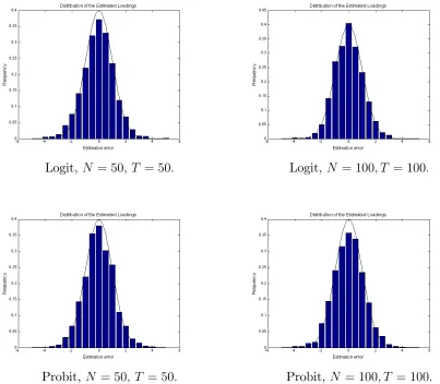
Due to limited space, we only present results for(N; T) = (50;50) and (100;100). According to Theorem 2,N12
1 2
t ( ^ft ftG) follows standard normal distribution10 for
each t and so does T12 1 2
iF(^i Gi ) for each i. Figure 1 displays the histograms
of N12 1 2
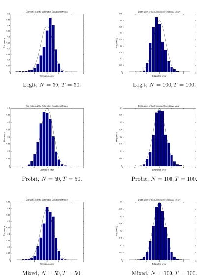
T =2; ( ^fT =2 fT =G2) for the three DGPs. Figure 2 displays the histograms of
T12 1 2
N=2;F(^N=2 G
N=2) for DGP1 and DGP2. For DGP3, Figure 3 displays the
his-tograms of T12 1 2
i;F(^i G
i ) for i = N=5, 3N=5 and 9N=10. The histograms are
normalized to be a density function and the standard normal density curve is over-laid on them for comparison. It is easy to see that in all sub…gures, the standard normal density curve provides good approximation to the normalized histograms. Note that for di¤erent sub…gures, the variance of the unnormalized estimation error, i.e., f^t ftG and ^i Gi , varies with N, T and DGP of xit. But once normalized,
the estimation errors always approximately follow the standard normal distribution. Also, the approximation is better asN andT increases from 50 to 100. These together lend strong support to the theoretical results.
Now we consider the factor-augmented regression, yt+1 = 0ft0 + 0Wt + t+1.
We already have f0
t and f^t. Wt is i:i:d:N(0;1) and is …xed down once generated.
f t+1; t = 1; :::; Tg is i:i:d:N(0;1) and generated 2000 times. For the regression
co-e¢cients, we choose = = 1. According to Theorem 4, (^yT+1jT yT+1jT)=BT
should follow standard normal distribution. Figure 4 displays its histograms for the three DGPs. As Figures 1-3, the standard normal density curve is overlaid on the normalized histograms. On the whole, standard normal distribution provides rea-sonable approximation. The slight skewness of the histograms for the Logit case disappears if we further increase N and T. Theorem 4 also allows constructing con-…dence intervals for the conditional mean yT+1jT and the one step ahead forecast.
The 95% con…dence interval is (^yT+1jT 1:96BT;y^T+1jT + 1:96BT) for yT+1jT and
10Note that here
iF = iF, t = t , and since ft and i are i:i:d:N(0;1) and N = T, we
Table 1: Coverage Rates of Con…dence Intervals
Logit Probit Mixed
N T y^T+hjT y^T+h y^T+hjT y^T+h y^T+hjT y^T+h
50 50 0.954 0.947 0.946 0.948 0.959 0.950 50 100 0.955 0.951 0.961 0.950 0.943 0.952 100 50 0.931 0.943 0.961 0.951 0.954 0.952 100 100 0.962 0.944 0.941 0.950 0.948 0.951
(^yT+1jT 1:96
p B2
T + 2;y^T+1jT + 1:96
p B2
T + 2) for the one step ahead forecast.
Table 1 reports the coverage rates for the three DGPs. In all cases, the coverage rate is close to the nominal level 95%.
8
Conclusions
Figure 1: Distribution of the Estimated Factors
Logit, N = 50; T = 50: Logit, N = 100; T = 100:
Probit, N = 50; T = 50: Probit, N = 100; T = 100:
Mixed, N = 50; T = 50: Mixed,N = 100; T = 100:
Figure 2: Distribution of the Estimated Loadings (Logit and Probit)
Logit, N = 50; T = 50: Logit, N = 100; T = 100:
Probit, N = 50; T = 50: Probit, N = 100; T = 100:
Figure 3: Distribution of the Estimated Loadings (Mixed)
Mixed (logit part), N = 50; T = 50: Mixed (logit part), N = 100; T = 100:
Mixed (probit part), N = 50; T = 50: Mixed (probit part), N = 100; T = 100:
Mixed (Gaussian part), N = 50; T = 50: Mixed (Gaussian part),N = 100; T = 100:
Figure 4: Distribution of the Estimated Conditional Mean
Logit, N = 50; T = 50: Logit, N = 100; T = 100:
Probit, N = 50; T = 50: Probit, N = 100; T = 100:
Mixed, N = 50; T = 50: Mixed,N = 100; T = 100:
References
[1] Bai (2003): “Inferential Theory for Factor Models of Large Dimensions,” Econo-metrica, 71, 135-171.
[2] Bai (2009): “Panel Data Models with Interactive Fixed E¤ects,”Econometrica, 77, 1229-1279.
[3] Bai and Li (2012): “Statistical Analysis of Factor Models of High Dimension,”
Annals of Statistics, 436-465.
[4] Bai and Li (2016): “Maximum Likelihood Estimation and Inference for Approx-imate Factor Models of High Dimension,” Review of Economics and Statistics,
98, 298-309.
[5] Bai and Ng (2002): “Determining the Number of Factors in Approximate Factor Models,”Econometrica, 70, 191–221.
[6] Bai and Ng (2006): “Con…dence Intervals for Di¤usion Index Forecasts and Inference for Factor-augmented Regressions,” Econometrica, 74, 1133-1150.
[7] Bartholomew (1980): “Factor Analysis for Categorical Data,” Journal of the Royal Statistical Society. Series B, 293-321.
[8] Bartholomew and Knott (1999): Latent Variable Models and Factor Analysis. Edward Arnold.
[9] Bernanke, Boivin and Eliasz (2005): “Measuring the E¤ects of Monetary Pol-icy: A Factor-augmented Vector Autoregressive (FAVAR) approach,”Quarterly Journal of Economics, 120, 387–422.
[10] Bohning and Lindsay (1988): “Monotonicity of Quadratic-approximation Algo-rithms,”Annals of the Institute of Statistical Mathematics, 40, 641–663.
[12] Chen (2016): “Estimation of Nonlinear Panel Models with Multiple Unobserved E¤ects,” Warwick Economics Research Paper Series.
[13] Chen, Fernandez-Val and Weidner (2014): “Nonlinear Panel Models with Inter-active E¤ects,” arXiv preprint arXiv:1412.5647.
[14] Chen, Fernandez-Val and Weidner (2018): “Nonlinear Factor Models for Network and Panel Data,” Cemmap Working Paper CWP38/18
[15] Collins, Dasgupta and Schapire (2001): “A Generalization of Principal Com-ponent Analysis to the ExCom-ponential Family,” Advances in Neural Information Processing System, Vol. 13.
[16] Cox and Reid (1987): “Parameter Orthogonality and Approximate Conditional Inference,” Journal of the Royal Statistical Society. Series B, 1-39.
[17] Creal, Schwaab, Koopman and Lucas (2014): “Observation-driven Mixed-measurement Dynamic Factor Models with an Application to Credit Risk,” Re-view of Economics and Statistics, 96, 898-915.
[18] de Leeuw (2006): “Principal Component Analysis of Binary Data by Iterated Singular Value Decomposition,” Computational Statistics & Data Analysis, 50, 21-39.
[19] Feng, Wang, Han, Xia and Tu (2013): “The Mean Value Theorem and Taylor’s Expansion in Statistics,” American Statistician, 67, 245-248.
[20] Fernandez-Val and Weidner (2016): “Individual and Time E¤ects in Nonlinear Panel Models with Large N, T,” Journal of Econometrics, 192, 291-312.
[21] Filmer and Pritchett (2001): “Estimating Wealth E¤ects without Expenditure Data—or Tears: An Application to Educational Enrollments in States of India,”
Demography, 38, 115-132.
[23] Hahn and Kuersteiner (2011): “Bias Reduction for Dynamic Nonlinear Panel Models with Fixed E¤ects,” Econometric Theory, 27, 1152-1191.
[24] Hunter and Lange (2004): “A Tutorial on MM Algorithms,”American Statisti-cian, 58, 30-37.
[25] Koopman and Lucas (2008): “A Non-Gaussian Panel Time Series Model for Estimating and Decomposing Default Risk,” Journal of Business & Economic Statistics, 26, 510-525.
[26] Koopman, Lucas and Monteiro (2008): “The Multi-state Latent Factor Intensity Model for Credit Rating Transitions,” Journal of Econometrics,142, 399-424.
[27] Koopman, Lucas and Schwaab (2011): “Modeling Frailty-correlated Defaults Using Many Macroeconomic Covariates,” Journal of Econometrics, 162, 312-325.
[28] Jennrich (1969): “Asymptotic Properties of Non-linear Least Squares Estima-tors,” The Annals of Mathematical Statistics, 40, 633-643.
[29] Joreskog and Moustaki (2001): “Factor Analysis of Ordinal Variables: A Com-parison of Three Approaches,” Multivariate Behavioral Research, 36, 347-387.
[30] Lancaster (2000): “The Incidental Parameter Problem since 1948,” Journal of Econometrics, 95, 391-413.
[31] Lancaster (2002): “Orthogonal Parameters and Panel Data,” Review of Eco-nomic Studies, 69, 647-666.
[32] Lange, Hunter and Young (2000): “Optimization Transfer Using Surrogate Ob-jective Functions,” Journal of Computational and Graphical Statistics, 9, 1-20.
[34] Moustaki (1996): “A Latent Trait and a Latent Class Model for Mixed Observed Variables,” British Journal of Mathematical and Statistical Psychology, 49, 313-334.
[35] Moustaki (2000): “A Latent Variable Model for Ordinal Variables,” Applied Psychological Measurement, 24, 211-223.
[36] Moustaki and Knott (2000): “Generalized Latent Trait Models,”Psychometrika, 65, 391-411.
[37] Newey and McFadden (1994): “Large sample Estimation and Hypothesis Test-ing,” Handbook of Econometrics, Vol. IV, 2111-2245.
[38] Ng (2015): “Constructing Common Factors from Continuous and Categorical Data,”Econometric Reviews, 34, 1141-1171.
[39] Ross (1976): “The Arbitrage Theory of Capital Asset Pricing,” Journal of Fi-nance, 13, 341–360.
[40] Schein, Saul and Ungar (2003): “A Generalized Linear Model for Principal Com-ponent Analysis of Binary Data,”Proceedings of the Ninth International Work-shop on Arti…cial Intelligence and Statistics.
[41] Schonbucher (2000): “Factor Models for Portfolio Credit Risk,” Bonn Econ Dis-cussion Papers 16.
[42] Stock and Watson (2002): “Forecasting Using Principal Components from a Large Number of Predictors,” Journal of American Statistical Association, 97, 1167–1179.
[43] Stock and Watson (2016): “Factor Models and Structural Vector Autoregressions in Macroeconomics,” Handbook of Macroeconomics, forthcoming.
Maximum Likelihood Estimation and Inference for High Dimensional
Nonlinear Factor Models with Application to Factor-augmented
Regressions
Appendix
A
Structure of the HessianSince @ P( G; fG) = 0, the score is
S = (XT
t=1@ l1tf
G0
t ; :::;
XT
t=1@ lN tf
G0
t ;
XN i=1@ li1
G0
i ; :::;
XN i=1@ liT
G0
i )0: (15)
For the Hessian, de…ne
HL( ) =
"
HL 0( ) HL f0( )
HLf 0( ) HLf f0( )
#
: (16)
and
JL( ) =
"
0 JL f0( )
JLf 0( ) 0
#
: (17)
HL 0( )is of dimensionN r N rand block-diagonal. Each block isr r and thei-th
diagonal block is PTt=1@ 2lit( it)ftf0
t. HLf f0( ) is of dimension T r T r and
block-diagonal. Each block is r r and the t-th diagonal block is PkN=1@ 2lkt( kt) k 0
k.
HL f0( ) is of dimension N r T r. Each block is r r and the (i; t) block is
@ 2lit( it)ft 0
i. HLf 0( )is the transpose ofHL f0( ). JL f0( )is of dimensionN r T r.
Each block is r r and the (i; t) block is @ lit( it)Ir. JLf 0( ) is the transpose of
JL f0( ). It follows that
@ 0L( ) =HL( ) +JL( ): (18)
LetHP( ) =@ 0P( ), then
H( ) =HL( ) +JL( ) +HP( ): (19)
Next, for p = 1; :::; r and q = p+ 1; :::; r, de…ne vp, upq and uqp as follows. Let vp
p-th element is ip and all the other elements are zeros. For the last T r elements, in
thet-th block, thep-th element is ftp and all the other elements are zeros. Let upq
be a N r+T r dimensional vector. The last T r elements are all zeros. For the …rst
N r elements, in thei-th block, the p-th element is iq, the q-th element is ip and all
the other elements are zeros. Let uqp be aN r+T r dimensional vector. The …rst N r
elements are all zeros. For the lastT r elements, in thet-th block, thep-th element is
ftq, the q-th element is ftp and all the other elements are zeros. Also, when = G
and f = fG, v
p, upq and uqp are denoted as vpG, uGpq and uGqp respectively. It can be
veri…ed that
@ [(
PN i=1
2
iq
N
PT t=1ftq2
T )
2] = 4(
PN i=1
2
iq
N
PT t=1ftq2
T )D
1
N Tvq;
@ 0[(
PN i=1
2
iq
N
PT t=1ftq2
T )
2] = 8D 1
N Tvqvq0DN T1
+4(
PN i=1
2
iq
N
PT t=1ftq2
T )D
1
N T(IN+T q);(20)
where q is anr rmatrix with theq-th diagonal element being one and all the other
elements being zero. Also,
@ 0[(
XN
i=1 ip iq)
2] = 2[u
pqu0pq+ (
XN
i=1 ip iq)D1]; (21)
@ 0[(
XT
t=1ftpftq)
2] = 2[u
qpu0qp+ (
XT
t=1ftpftq)D2];