Encoding Lexicographical Ordering Constraints in SAT

Illinois Wesleyan University

Digital Commons @ IWU

Honors Projects

Computer Science

2017

Encoding Lexicographical Ordering Constraints in

SAT

Wenting Zhao

Illinois Wesleyan University

This Article is brought to you for free and open access by The Ames Library, the Andrew W. Mellon Center for Curricular and Faculty Development, the Office of the Provost and the Office of the President. It has been accepted for inclusion in Digital Commons @ IWU by the faculty at Illinois Wesleyan University. For more information, please [email protected].

Recommended Citation

Zhao, Wenting, "Encoding Lexicographical Ordering Constraints in SAT" (2017).Honors Projects. 21. https://digitalcommons.iwu.edu/cs_honproj/21

Encoding Lexicographical Ordering Constraints

in SAT

Wenting Zhao

Illinois Wesleyan University, Bloomington IL 61701, USA [email protected]

Abstract. Symmetry occurs in many constraint satisfaction problems, and it is important to deal with it efficiently and effectively, as it often leads to an exponential number of isomorphic assignments. Symmetric rows and columns in matrices are an important class of symmetries in constraint programming. In this work, we develop a new SAT encoding for partial lexicographical ordering constraints to break symmetries in such places. We also survey all the previous complete lex-leader encod-ings in literature and translate them into SAT encodencod-ings. We perform experimental analysis on how these lex-leader constraints impact the solving of Balanced Incomplete Block Design (BIBD) instances. Each encoding is able to outperform the other encodings on some instances, and they all perform close to each other; no clear winner can be drawn. Finally, the result shows that though using any lex-leader constraints is detrimental to finding a single BIBD, they are necessary in enumerating all BIBDs and proving non-existing designs.

1

Introduction

The phenomenon of symmetry arises in many constraint satisfaction problems (CSPs), such as scheduling, configuration, and design problems. A common form of symmetry is the interchangeability between elements of sets of variables and between elements of sets of of values. Breaking symmetry reduces the search space, which may in turn improve performance. In this paper, we focus on one class of symmetries in constraint programming: row and column symmetries in matrix models, which are constraint programs that contain matrices of Boolean variables [6]. A common way to break symmetries in a constraint satisfaction problem is to generate extra constraints to prevent some assignments from being returned.

For example, there can be column and row symmetries in a Latin square, which is an n·n matrix filled withn different symbols. Given a Latin square, where every symbol occurs exactly once in each row and exactly once in each column, any permutation of the columns or rows will simply map that Latin square to an equivalent Latin square. Adding constraints to enforce lexicographic (lex-leader) ordering on the columns and the rows can eliminate some equivalent Latin squares. By asking a solver to only return the Latin squares of a given ordernin lex-leader, we break symmetries between rows and between columns.

If we ignore symmetries in the solution set, computing resources will be wasted to consider symmetric but essentially equivalent assignments, and for an assignment there could be an exponential number of equivalent assignments. This could become incredibly costly, and hence breaking symmetries is important to reduce the search space, thus avoiding redundant work.

Such constraints can be expressed in satisfiability modulo theories (SMT). Examples of such theories are the theory of real numbers, the theory of integers, and the theories of various data structures such as lists, arrays, bit vectors and so on. As SMT contains a wide range of theories, it is very expressive of encoding constraints. Many ways have been developed in SMT to produce constraints for enforcing lex-leader when solving a problem (for a survey, see [5]). However, there has been little study on breaking symmetries using lex-leader constraints in Boolean Satisfiability (SAT), which can only be formulated by propositional logic, thus providing less expressive encoding of a problem. In [10], the authors showed that developing problem-specific symmetry breaking, which depends on application domains, is much more efficient than using generalized symmetry breaking, which can be applied to any propositional formulas; in this case, the specific problem is the problems that can be modeled using matrices of decision variables.

Given a problem, SMT can generally encode it in a more expressive way, whereas SAT has less expressive encoding, but SAT solvers are often considered much more efficient to use than SMT solvers. A naive way to encode lex-leader in SAT would result in quadratically many additional constraints (with regards to the number of bits in the variable vector), hence largely increasing the sizes of the problems people intend to solve. In this paper, we propose a new way to encode partial lex-leader in SAT, aiming to benefit from both a compact encoding and an efficient solver. Numerous papers were published to present different encodings for lex-leader constraints in SMT, and some ways may work better for some problems while the others are better-suited for other problems. Hence, we also translate all the previous lex-leader encodings from SMT to SAT, and then we evaluate the new partial lex-leader encoding and all the previous ones on a large set of design problems, known as the balanced incomplete block designs (BIBDs) problem. Counter-intuitively, we show that, although the new encoding generates fewer constraints and no extra time is needed for getting the formulas into a proper form to be processed by SAT solvers, the new encoding is significantly slower than all the previous encodings. Finally, we also conclude that symmetry breaking is key to enumerating all BIBDs for a given order and proving the non-existence for the problem when such a design does not exist.

2

Preliminaries & Background

We first introduce the definition of the Boolean Satisfiability Problem. A Boolean variable can either be assignedtrueorfalse. Throughout the paper, we will treat all Boolean variables as 0/1 variables, where the value 1 represents True and the value 0 represents False. A propositional formula is defined over a set of

variables of logical values, operators AND (conjunction, also denoted by∧), OR (disjunction, ∨), NOT (negation, ¬). A propositional formula F is said to be

satisfiable if there exists an assignment to all variables that makes F evaluated to be 1; otherwise, we sayF isunsatisfiable. TheBoolean Satisfiability Problem (SAT) is, given a propositional formula, to determine whether it is satisfiable. A SAT solver is a program that takes a propositional formula as an input and produces an answer whether or not the given formula is satisfiable; if yes, then the solver returns a proof – an assignment by which the formula is evaluated 1. A standard SAT solver only takes the propositional formulas of a special form as input, which is known as conjunctive normal form (CNF). If a propositional formula is not in CNF, then we need to do some translation before it is passed to a SAT solver to solve. A propositional formula F is said to be in CNF if it is a conjunction of clauses, F = V

i=1..nCi; each clause Ci is a disjunction of

literals, Ci=li1∨li2∨ · · · ∨liki; and each literal is either a Boolean variablex

or its negation¬x. Consider the following formula ϕ: ϕ= (a)∧(¬b)∧(¬a∨ ¬c)

ϕconsists of three Boolean variables and three clauses where the first two clauses are unit and the following one clause is a disjunction of two variables. A satisfying assignment to the above formulaϕisa= 1, b= 0, c= 0. Thus,ϕis satisfiable.

A matrix model is a representation of a combinatorial problem as a matrix of Boolean variables with constraints on the allowed assignments to those variables. A solution symmetry in such a model is a permutation of the set of variable-value assignments that preserves the set of solutions; that is, an assignment is a solution to the matrix iff its symmetry is a solution to the matrix as well. In a matrix model, there are often many solution symmetries to an assignment. Symmetry occurs because there are cases where the columns/rows within the model are indistinguishable from each other. Thus, permuting indistinguishable rows (resp. columns) in an assignment will generate equivalent assignments. Breaking symmetries is crucial in reducing the search space, as there may be exponentially many equivalent assignments to one assignment in a matrix, and exhaustively checking every one of them is computationally expensive. Ideally, we want a solver to only return one solution from a set of equivalent solutions. Thus, to break symmetries is to help a solver to identify one out of many.

One common way to accomplish symmetry breaking is to order the symmetric objects. To break row or column symmetry, we can simply impose lexicographi-cal order on rows or columns. With each row treated as a 0/1 vector, we say that the rows in a matrix are lexicographically ordered if each row is lexicographi-cally equal to or greater than any of the previous rows. Similarly, with each column treated as a 0/1 vector, we say that the columns in a matrix are lexico-graphically ordered if each column is lexicolexico-graphically equal to or greater than any of the previous columns. We place constraints on the row and the column vectors, so that they can be ordered lexicographically; we call the constraints

lex-leader constraints. By adding these constraints, many assignments that pre-viously solved the problem would no longer be valid solutions, as they falsify the

newly-added symmetry breaking clauses. Note that adding symmetry breaking predicates would not change the satisfiability of a problem instance, since, if a satisfying assignment exists, we can always reorder the columns and rows to get that assignment in lexicographical order.

3

Previous Work: Lex-Leader Constraints

There are nine existing lex-leader encodings that were proposed in the field of SMT; however, we can only encode eight of them in SAT with a reasonable amount of modifications. The ninth encoding involves exponential calculations that will result in too many clauses when translated into SAT. We thus only consider eight of the nine existing SMT encodings of lex-leader constraints in the later experimental comparison.

Throughout, we consider a non-strict lex-leader constraint between two 0/1 vectorsM andN with each bit being a Boolean variable. The two vectors must have equal length, which we will denoten, andn≥2. The lex-leader constraints we are going to produce in each of the following encodings ensures the vector M is lexicographically greater than the vectorN. Furthermore, in propositional logic, for any two Boolean variablesxandy,x≥y is equivalent tox∨ ¬y, and x > y is equivalent tox∧ ¬y; we will be using both of these translations in the following discussion. We also note that in the rest of this section, the lines of formulas are connected by the logic operator∧.

3.1 The AND Encoding [7]

The AND encoding says that if all the pairs of bits fromM[1] and N[1] up to and including M[i] and N[i] are equal, then for the next pair of bits M[i+ 1] and N[i+ 1], the former has to be greater than or equal to the latter in order to maintain the lexicographical order. And this has to be true for everyiwhere 1≤i≤n−1. The lex-leader constraints are constructed as follows:

M[1]≥N[1] n−1 ^ i=1 ( i ^ j=1 M[j] =N[j])→(M[j+ 1]≥N[j+ 1])

For example, to enforce lexicographical order on vectorsM andN with each of them containing five bits, by applying this AND encoding, we get the following formulas: M[1]≥N[1] (M[1] =N[1]) →(M[2]≥N[2]) (M[1] =N[1])∧(M[2] =N[2]) →(M[3]≥N[3])

(M[1] =N[1])∧(M[2] =N[2])∧(M[3] =N[3]) →(M[4]≥N[4]) (M[1] =N[1])∧(M[2] =N[2])∧(M[3] =N[3])∧(M[4] =N[4]) →(M[5]≥N[5]) Note that there are 15 occurrences of atoms in the above formula. For gen-erating lex-leader constraints by the AND encoding in general, the size of the lex-leader formula grows quadratically as the number of bits increases; the num-ber of atoms in this encoding is n2₂+n.

3.2 The AND Encoding using Common Subexpression Elimination [5]

As we have seen in the previous AND encoding, the size of the formula grows rapidly when we have longer vectors. The AND encoding incorporating com-mon subexpression elimination (AND-CSE) was thus proposed to reduce the formula size by substituting any recurring parts of the formula with auxiliary variables. To generate this type of encoding, we create additional Boolean vari-ables,X[1]...X[n−1], such that

M[1]≥N[1] X[1]↔(M[1] =N[1]) ∀1≤i≤n−2, X[i+ 1]↔ X[i]∧(M[i+ 1] =N[i+ 1]) ∀1≤i≤n−1, X[i]→(M[i+ 1]≥N[i+ 1])

The first constraint ensures that the first pair of bits is lexicographically ordered. The second constraint relates the first auxiliary variable with the first pair of bits saying that X[1] is set to 1 if and only if M[1] =N[1]. The third constraint links the rest of the auxiliary variable to the bits in the vectors: a auxiliary variable is set to 1 if and only if the previous auxiliary variable is 1 and the corresponding pair of bits are equal. The last constraint is an implication that if an auxiliary variable is 1, then the pair of bits next to the current pair is M[i+ 1]≥N[i+ 1].

It works essentially the same as the original AND encoding, but it reduces the number of atomic formulas by applying the idea of induction. The second constraint serves as the base case, and the third constraint operates like the inductive step that the equality of each current pair is based on the equality of the previous pair of bits. Hence, any auxiliary variableX[i] is 1 if and only if the previous pairs of bits are equal. AndX[i] being 1 ensures M[i+ 1]≥N[i+ 1]; any pair ofM[i+ 1] andN[i+ 1] fails to satisfy that property means that there is already a previous pair of bits assures the lexicographical order.

Again, we look at the same example we presented above. To encode vectorM is lexicographically greater than vectorN, we produce the following constraints:

M[1]≥N[1] X[1]↔(M[1] =N[1]) X[2]↔ X[1]∧(M[2] =N[2]) X[3]↔ X[2]∧(M[3] =N[3]) X[4]↔ X[3]∧(M[4] =N[4]) X[1]→(M[2]≥N[2]) X[2]→(M[3]≥N[3]) X[3]→(M[4]≥N[4]) X[4]→(M[5]≥N[5])

The above formula contains 20 atomic formulas. In general, encoding lex-leader constraints by using the AND-CSE encoding produces 5n−5 occurrences of atoms.

3.3 The OR Encoding [7]

We then introduce the OR encoding. This one exhaustively lists all the possibil-ities of how two vectors can be lexicographically ordered and uses disjunctions to connect them. The following are the possible assignments maintaining lexico-graphical order between the two vectorsM andN:

1. M and N differ in the first bit: the first bit of M is 1 and the first bit of N is 0. By then,M is already lexicographically greater thanN, and it does not matter what the seconds bits of those vectors are.

2. M and N have the same first bits and differs in the second bits with the second bit ofM being greater than that ofN, or first two pairs of bits inM andN are equal and differs in the third bits with the third bit ofM being greater than that ofN, and so on.

3. M andN are equal: every pair of bits in M andN has the same value. The formulas for this encoding are set out as follows:

C1 = (M[1]> N[1]) C2 = n−1 _ i=1 i ^ j=1 M[j] =N[j] C3 = n ^ i=1 (M[i] =N[i])

C1∨C2∨C3

They are all valid ways of assigningM to have a greater lexicographical value than N, so we use disjunctions to connect them. Once any part of the big OR is satisfied, then the whole lex-leader constraints are satisfied. This encoding consists of n2+15₂ n atomic formulas, and hence it has the same complexity as the AND encoding has. If the vectors are large, then encoding lex-leader constraints this way will not scale well, as they may lead to excessive memory usage.

3.4 The OR Encoding using Common Subexpression Elimination [5]

Similar to the AND encoding using common subexpression elimination, we can reduce occurrences of atoms by replacing the recurring parts by auxiliary vari-ables. Additional variables X[1]...X[n] are created to avoid repeating patterns in the OR encoding. X[1]↔(M[1] =n[1]) ∀1≤i≤n−1, X[i+ 1]↔ X[i]∧(M[i+ 1] =N[i+ 1]) (M[1]> N[1])∨ n−1 _ i=1 X[i]∧(M[i+ 1]> N[i+ 1]) ∨X[n]

X[i] implies that for all previous pairs associating to 1...i, the two bits in each pair are equal to each other, and vice versa; this relation is established by the second constraint. The first constraint serves as a base case for this relation, stating thatX[1] is 1 if and only ifM[1] andN[1] have the same value. Finally, the third constraint exhaustively lists all possible ways of having vector M to be lexicographically greater than or equal to vector N by using the auxiliary variables which makes use of the common subexpression. There are 13n−7 occurrences of atoms in this encoding.

3.5 The Recursive OR Encoding [8]

Alternatively, the OR encoding can be constructed recursively as follows.

(M[1]> N[1])∨(((M[1] =N[1])∧(M[2]> N[2]))∨((M[2] =N[2])∧(...∧(M[n]≥N[n])...)))) However, in order to programmatically build up such a recursive formula, we

need to convert it to a iterative form, as a SAT solver will not be able to parse it. The following constraints are thus used to form the recursive OR encoding, withX[1]...X[n]

X[1]

∀1≤i≤n−1, X[n−i]↔

M[n−i]> N[n−i]∨(M[n−i] =N[n−i]∧X[n−i+1])

X[1] is defined to be true, andX[n] is set to 1 if and only if M[n]≥N[n]. The recursion goes from the bottom of the vectors to the top. Starting from the second last pair of bits in the vectors M and N, the third constraint says that X[n−1] is 1 if and only if for the second last pairM[n−1]≥N[n−1] holds or they are equal butX[n−2] is 1. This process applies again toX[n−2], and so on and so forth to X[2], and thus it covers every possible assignment that preserves the lexicographical order between the vectorsM andN. This recursive OR encoding results in 2natomic formulas.

3.6 The Harvey Encoding [7]

The Harvey lex encoding is a recursive arithmetic encoding:

(N[1]<(M[1] + (N[2]<(M[2] + (...+ (N[n]<(M[n]) + 1)...)))) = 1 The 1 on the right-hand side of the formula means the left-hand side has to be evaluated 1. LetP be a vector of bits; we defineP[x:y] to be a sub-vector ofP starting inclusively at thexth bit and ending inclusively at theyth bit. To understand this encoding, we look at one recursive step - the first recursive step:

M[1 :n]≥lexN[1 :n]≡N[1]<

M[1] + (M[2 :n]≥lex N[2 :n])

The part underlined in the first formula in this section was turned into the recursive callM[2 :n]≥N[2 :n], which is equivalent toM andN starting bits 2 and on are lexicographically ordered. We also generate the truth table of the above formula:

Table 1.Truth table for the first recursion step in the Harvey encoding

M[1]N[1]M[2 :n]≥lexN[2 :n]M[1 :n]≥lexN[1 :n] 0 0 0 0 0 0 1 1 0 1 0 0 0 1 1 0 1 0 0 1 1 0 1 1 1 1 0 0 1 1 1 1

We can see from the table that, whenM[1] andN[1] have the same value, it will then depend on if M[2 : n] ≥lex N[2 : n] holds. In other words, if

M[1] =N[1], then M[1 :n]≥lex N[1 :n] if and only if M[2 :n]≥lex N[2 :n].

formula is determined immediately; thatM[1 :n]≥lexN[1 :n] is 1 immediately

follows from M[1] > N[1], and similarly, that M[1 : n] ≥lex N[1 : n] is 0

immediately follows fromM[1]< N[1].

To translate this recursive construction into propositional logic, the following formulas are utilized:

X[1] X[n]↔ N[n]<(M[n] + 1) ∀0≤i≤n−2, X[n−i−1]↔ N[n−i−1]>(M[n−i−1] +X[n−i])

An array of auxiliary variables,X[1]...X[n], is needed to complete the con-struction.X[i] is 1 if and only if the sub-vectorsM[i:n]≥lexN[i:n], and hence

the first constraint guarantees that vectorM is lexicographically larger thanN, the second constraint serves as a base case, and the third constraint completes the recursive step. This formulation of encoding lex-leader constraints produces 2n−1 occurrences of atoms, hence maintaining fairly small formula sizes.

Finally, in order to express the third constraint in CNF, we need to do some translation. The right-hand side of the constraint, in the form A > B+C, can be converted to (B∨C)∧(¬A∨B)∧(¬A∨C) by completing a truth table for the formula and producing a Boolean expression in minimal product-of-sums form via a Karnaugh map.

3.7 The Alpha Encoding [8]

In the encoding, we use an array of auxiliary Boolean variables, α[1]...α[n], to keep track of the relations between values, thus calling it the Alpha encoding. Theαarray is defined to behave as follows: for 1≤i≤n, 1≤j≤i, ifα[i] = 1 thenM[j] =N[j], if (α[i] = 1 andα[i+ 1] = 0) thenM[i+ 1]> N[i+ 1]. Hence, when α[i] = 0, every pair of bits indexed up to and includingi are guaranteed to be equal to each other. And note that forα[i] = 1 andα[i+ 1] = 0, the pair of bits indexedi+ 1 would be the first pair of bits where the bits differ. Hence, we make an implication ensuring that when the two conditions hold, M[i+ 1] must be greater thanN[i+ 1] and not the other way around. The following is the encoding incorporating the definition of theαarray.

α[0]

∀0≤i≤n−1, α[i+ 1]→α[i] (equiv. to¬α[i]→ ¬α[i+ 1])

∀1≤i≤n, α[i]→(M[i] =N[i])

∀0≤i≤n−1, α[i]∧(¬α[i+ 1]) →(M[i+ 1]> N[i+ 1]) ∀0≤i≤n−1, α[i]→(M[i+ 1]≥N[i+ 1])

The first constraint together with the fifth one guarantees M[1]≥ N[1]. If α[i] = 1, then by the second constraint it follows that all the elements from α[0]...α[i−1] are all equal to 1; thus, all pairs indexed up to and including i are equal to one another. This encodes the first part of the α array definition, and the fourth constraint directly follows from the second part of the definition. The number of atoms generated in the above formulas is 9n−6, growing linearly as the number of bits in a vector increases. Notice that this Alpha encoding behaves very similar to the AND encoding in a way that they both focus on the pair of bits in which the bits first differ from each other, but the second and the fourth constraints in the Alpha encoding have made the pair of bits after first occurrence ofM[i]> N[i] unimportant – all the elements after index iin the αarray is then 0 by the second constraints, and so the implication in the fourth constraint will no longer be triggered. However, the above information is not explicitly expressed in the AND encoding.

3.8 The Alpha M Encoding [2]

The Alpha M encoding evolved from the Alpha encoding, also using theαarray to keep track of the relation between pairs of bits. It is constructed as follows:

α[1]

∀1≤i≤n, α[i]↔

((M[i]> N[i])∨α[i+ 1])∧(M[i]≥N[i])

The Alpha M encoding uses the same underlying mechanism to encoding lex-leader constraints; however, unlike the Alpha encoding where eachα[i] only implies the relation between the current pair of bits and affects the relation between the next pair of bits by affecting α[i+ 1], the Alpha M encoding in-tegrates all of the above into a single constraint. Now, α[i] being 1 guarantees that M[i]≥N[i] holds, and further, if M[i] =N[i], thus notM[i]> N[i], then it will forceα[i+ 1] to be 1 to satisfy the conjunction.

The first constraint α[1] ensures M[1] ≥ N[1], and if M[1] = N[1], then α[2] = 1. And this would continue until the first pair of bits whereM[i]> N[i] appears; then, the value of α[i+ 1] becomes insignificant. Onwards, the later elements in theαarray can either be 0s or 1s, but there are no longer constraints forcing them to be one way or the other. There are 4n+ 1 atomic formulas in this encoding, maintaining the linear growth rate of the sizes of the formulas.

4

New Lex-Leader Constraints

In the earlier work, the constructions of lex-leader constraints either come with very large formula sizes or need auxiliary variables to make them work, with the former more likely leading to exhausted memory while running SAT solvers and the latter increasing the time complexity to solve the augmented formulas. Furthermore, the previous encodings cannot be directly expressed in CNF; they

need to be first written in some general propositional formulas and then be translated to CNF. In this paper, we propose a new way of encoding lex-leader constraints which only consists of implications and does not require additional variables. Most importantly, this encoding can be directly written in CNF; thus, it saves the time from doing the CNF translation. However, this encoding only ensures partial lex-leader, which we will discuss in detail later in this section.

4.1 The Original Construction

We start from our original construction, which has a quadratic number of clauses attached to an implication and is extremely inefficient to solve. The following example offers an overview of this construction, in which we build partial column lex-leader. It is a matrix with five columns and four rows; we assign the cells (2,1) and (2,2) to be 0s and the cell (3,3) to be 1.

Table 2.An example to show how the column lex-leader is maintained by applying the lex-leader constraints.

1 2 3 4 5

1 00 0

2 00 0

3 1

4

Our encoding works as follows: on the column indexed 3, starting from the top, there are two 0s followed by a 1; then, the four cells on the later columns above the 1 are all propagated 0 in order to maintain lexicographical ordering. If we place a 1 in any of the four cells, say v4,1 = 1, then the column indexed 4 will be lexicographically greater than the column indexed 3, and thus the full lexicographical descending order in this matrix is invalid.

We then write out the formal construction in propositional formulas. We number the columns of a matrix to be 1...cand the rows to be 1...r; the variable vi,j represents the cell on the column indexediand the row indexedj; it can be

of value either 0 or 1. We make the following lex-leader constraint for every cell (x, y) in the matrix to ensure all the columns are in lexicographical descending order: ^ j=1..x−1 ¬vy,j ∧vy,x → ^ i=y+1...c ^ j=1...x−1 vi,j

Looking at the formula, we can see that once a cell is assigned 1 with all the cells above on the same column being 0s, then the cells above that cell on the later columns (i.e., on its top-right side) will all be propagated 0s. This is correct because all the columns are ordered lexicographically descendingly, all the later columns to the column should have smaller lexicographical values than

that column’s, and a 1 on any of the later columns that is above that cell will immediately lead to a greater lexicographical value. Therefore, the cells in the top-right region all have to be 0s in order to maintain such a descending order. Similarly, we can use the same idea to generate row lex-leader constraints; for every cell (x, y) in the matrix:

^ i=1..y−1 ¬vi,x ∧vy,x → ^ j=x+1...r ^ i=1...y−1 vi,j

When a cell is assigned 1 with all the previous cells on the same row being 0s, then the cells below that cell on the later rows (i.e., on its bottom-left side) will all be propagated 0s. Any of the cells in the bottom-left region being 1 would make the corresponding row to have a greater lexicographical value than that of the earlier row, thus breaking the lexicographical descending order on the rows. We should note that this only encodes partial lex-leader in the sense that given two vectorsM andN, it only guarantees that there are no 1s starting the first bit inN until the first time when 1 occurs inM; if the bit inN is also 1 at the place where 1 first occurs inM, then M andN are lexicographically equal thus far, and N could turn out to be greater thanM in the later bits. Hence, there is no guarantee for complete lex-leader between the two vectors.

Further, notice that we can combine the row and the column lex-leader con-straints in a single matrix to break the column and row symmetries at the same time; however, the lex-leader constraints should be encoding either both the as-cending order or both the desas-cending order. Otherwise, having the rows being in ascending order and the columns being in descending order, or vice versa, will lead to incorrect results: this may eliminate some non-isomorphic satisfying assignments to the original formula, since for every assignment the correspond-ing rows and columns can always be reordered to be lexicographical in the same direction but not in the opposite directions.

4.2 The Optimized Construction

The original encoding is extremely inefficient, in that there are many recurring parts. For every implication to be written in CNF, every cell that is implied is in an individual clause. Again, let us look at the example above again. The whole implication is accomplished by four clauses:

v3,1∨v3,2∨ ¬v3,3∨v4,1 v3,1∨v3,2∨ ¬v3,3∨v4,2 v3,1∨v3,2∨ ¬v3,3∨v5,1 v3,1∨v3,2∨ ¬v3,3∨v5,2

As each clause is composed purely of ORs, we are not able to just write (v3,1∨v3,2∨ ¬v3,3)∨(v4,1∧v4,2∧v5,1∧v5,2), and hence v3,1∨v3,2∨ ¬v3,3 is

repeated many times, taking up much memory space. We thus aim to reduce the number of times that this part is repeatedly used.

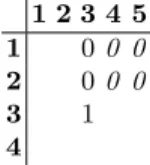
One way to achieve this is, instead of propagating 0s in all the later cells, we only propagate the cells in the very next column/row. The following table illustrates how this works:

Table 3.An example to show how the column lex-leader is maintained in the optimized construction. 1 2 3 4 5 1 00 2 00 3 1 4

We can see from the example that only the cells in the column next to the “assigned” column are propagated, but not all the later columns.

To formalize the construction, the column lex-leader constraints are as fol-lows: ^ j=1..x−1 ¬vy,j ∧vy,x → ^ j=1...x−1 vy+1,j

Going back to the example above, the cells on the column indexed 2 only imply the cells on the column indexed 3, and therefore the last two clauses are no longer needed, thus reducing the number of clauses needed by half. This is sound because for every pair of consecutive columns, the new column lex-leader constraints make sure that the former is lexicographically greater than the latter. Hence, the first column is greater than the second, the second is greater than the third, and so on. Every column is then lexicographically smaller than the previous column, and therefore all the columns are in lexicographical descending order.

And this applies to the rows, too:

^ i=1..y−1 ¬vi,x ∧vy,x → ^ i=1...y−1 vi,r+1

Starting from the beginning of a row, if there are a number of 0s followed by a 1, then only the cells on the very next row that go before the 1 cell are propagated. The memory space is hence saved by not having to imply the cells on all the later rows. Because these row lex-leader constraints force every row to be less than its previous row, the global row lex-leader is maintained. Again, these column and row lex-leader constraints can be combined to break both column and row symmetries in a matrix.

This encoding is much simpler than all the previous encoding in the following ways:

1. it does not need additional variables.

2. there are no comparisons between a pair of bits needed, and only implications are used; due to this simple structure, the encoding can be directly written in CNF, and no extra translations from a general propositional formula to its CNF are required.

However, again, the above bullets are in sacrifice of having a complete lex-leader encoding.

5

Encoding BIBDs into SAT

In this work, we will be analyzing experimentally the effectiveness of all the lex-leader encodings on the problem of finding balanced incomplete block designs (BIBDs), as it stands as a central and classic problem in the field of design theory. This section will be discussing the SAT encoding of such problem and identifying symmetries in our problem formulation. A hv, b, k, r, λi-BIBD is an assignment ofvdistinct points intobblocks, such that each block contains exactlykdistinct points, each point is used in exactlyrdifferent blocks, and every pair of distinct points is used in exactly λ blocks. Note that we do not need every parameter above to fully describe a BIBD. The three parametersv,k, andλare enough to uniquely identify a BIBD, and the rest can be calculated by

b= v 2 ×λ k 2 and r=v−1 b−1

Hence, in this paper, we will refer to ahv, b, k, r, λi-BIBD as av-k-λfor brevity. To encode this problem into a propositional formula, we create a b by v matrix and fill it with Boolean variables. Blocks correspond to columns, which are numbered 1 through b, and distinct points correspond to rows, which are numbered 1 throughv. A cell (i,j) is set to 1 if and only if the pointj is used in theith block. A valid design corresponds to a matrix whose variables satisfy the following constraints:

1. on each column, there are exactlykcells which are set to 1. 2. on each row, there are exactlyr cells which are set to 1

3. In addition to the variables in the matrix, we also create a variable for each distinct pair of points in a block, and we collect all the variables representing the same pair across every block and say there are exactlyλof them which are 1.

While the constraints above can be written using standard propositional formulas in CNF, it is often more efficient to use special purpose cardinality constraints, or counting constraints, which impose a bound on the number of

literals in some set that can be assigned the value 1. Given a set of n literals

{a1, a2, . . . , an}and an integer boundk, s.t. 0≤k≤n, a cardinality constraint

is defined as:

n

X

i=1 aiRk

where _R is any relation from the set {≤,=,≥}, forming AtMost, Equals, and

AtLeast constraints, respectively. Though we will be using these cardinality con-straints in our encoding of BIBDs for the purpose of compact encoding and efficient solving, we do not differentiate these SAT+cardinality instances from SAT instances for brevity.

In our problem representation for finding BIBDs, each block is numbered, and any permutation of all the blocks will yield an equivalent solution. Similarly, each point is numbered, and any permutation of the set of distinct points will yield an equivalent solution. Therefore for any solution to a BIBD problem, generating all column permutations produces b!−1 equivalent solutions and generating all row permutations produces v!−1 equivalent solutions. As there are an exponential number of symmetric solutions, producing them all would be extremely expensive and a waste of resources. Thus, we use the lex-leader constraints to break symmetries in rows and columns.

6

Results

We investigated the performance of the proposed lex-leader encoding and all the previous lex-leader encodings. We collected benchmarks from the table of BIBDs with Small Block Size in the Handbook of Combinatorial Designs [3]. This table is a comprehensive list of 140 BIBDs; some of these BIBDs exist, while the others do not. For the BIBDs where such designs do not exist, we test how fast their non-existence can be determined. We encode each of the BIBDs into SAT constraints by using the methodology described in the previous section, and each instance is the original problem constraints plus lex-leader constraints of a given type applied to both rows and columns. With our BIBD encoding, the resulting instances are ranging from 7203 to 4.7 million variables and from 994 constraints to 24 million constraints. The experiments were run on a Linux cluster with an Intel Core i5-2500 quad-core 3.3GHz (up to 3.7GHz turboboost) processor and 16GB of RAM per node. Every run was given a 3600 second timeout and a 3000 MB memory limit. From the benchmark set, we excluded from our analysis the 211-15-1 BIBD instance for which encoding the problem instance itself went over the memory limit. We then are left with 139 instances in total. We solved the SAT instances with cardinality constraints arising from these encodings with the MiniCard constraint solver [9], an extension of MiniSat [4] that handles cardinality constraints natively (i.e., as opposed to encoding them into CNF).

During the experiments, we recorded the runtimes for each step, including generating lex-leader constraints, translating those constraints to CNF, and gen-erating BIBDs. In this section, we first analyze the phase of gengen-erating lex-leader

constraints and how much it costs to transform a general propositional formula to its CNF. We also look at how many additional clauses were generated in addition to the original constraints from the problem itself, since an excessive amount of extra clauses could potentially outweigh any benefits breaking symmetries may provide. We then investigate the performance of solving the instances with each type of lex-leader constraint. We look at both producing a single result and enu-merating all results for a BIBD problem to see study how symmetry breaking affects the performance.

6.1 Producing Lex-leader Constraints + CNF translations

We start with the number of BIBD instances each encoding was able to produce the lex-leader constraints for within the given time and the memory limits. We refer to all the previous encodings by their names used in Section3, and the new partial lex-leader encoding we developed is denotedPartial-lex. All the encodings except for Partial-lex were able to generate the lex-leader constraints for all 139 instances; Partial-lex only produced lex-leader constraints for 134 instances, and for the other five instances the solver ran out of memory and was terminated by the operating system. Since the step of producing lex-leader constraints is steadily less than 1% of the total runtime, we do not further present how long this step actually took given how quickly they can be generated.

We then focus on the CNF translation; Table 4 shows how fast the lex-leader constraints produced by each encoding were translated to their CNF. For this step, we use bool2cnf[1], which takes any propositional formula as input and produces its CNF as output using the algorithm proposed by Plaisted and Greenbaum [11]. The worst-case runtime of that algorithm isO(n∗l), where n is the number of variables in the propositional formula, and l is length of the formula when expressed as a character string. Compared to SAT solving with an exponential worst-case runtime, this CNF translation is expected to be a small part of the total runtime, which is supported by the following data.

We first generate the lex-leader constraints in our own program, pass the outputs tobool2cnf, and add the resulting CNF formulas as a set of clauses to the MiniCard solver. We time the execution of bool2cnf in each instance and record it as the amount of time needed for the CNF translation. The first three rows in the table represents how long it took to translate lex-leader constraints to CNF for the instances where the CNF translation was finished, the fourth row sums up the first three rows, and the last row shows how many instances did not complete this step.

First, for all the encodings, there are some instances where the generated lex-leader constraints could not be converted to CNF; this is due to a “too many variables” error was raised during the execution of bool2cnf. And this error explains all the instances on the last row whose lex-leader constraints were generated but CNF was not produced. A variable limit was set in that program, and hence it failed to produce the formulas in CNF for those instances whose variables went over that limit. Since the encodings other than AND and OR all use additional variables, their resulting formulas have more variables than the

Table 4.Reporting statistics for CNF translation.

AND AND-CSE OR OR-CSE ROR Alpha Alpha-M Harvey

<1s 40 77 35 74 70 69 70 66

1s∼10s 52 25 55 28 32 32 31 36

10s∼100s 32 0 34 0 0 0 0 0

total-produced 125 102 124 102 102 101 101 102

not-produced 14 37 15 37 37 38 38 37

formulas generated by AND and OR; thus, AND and OR ran into the “too many variables” error fewer times than the other encodings, and more instances whose lex-leader constraints were generated by them can be converted to CNF. We can see from the table that, although more instances encoded by AND and OR can be converted to CNF, transforming the lex-leader constraints encoded in these two forms were slower than those produced by the other encodings. While for the rest of the encodings most of the instances fell in the first category of less than a second, most instances accumulated in the second category of 1-10 seconds for the AND and the OR encodings. Hence, we conclude that to translate the lex-leader constraints produced by these two encodings were significantly slower than translating the lex-leader constraints produced by the other encodings.

Let the number of clauses in the original problem instance be k, and the number of lex-leader clauses ben. Letr=n+k

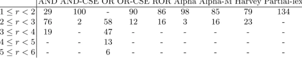
k ;rshows how many more clauses

were generated with regards to the number of original constraints. A larger r value means more clauses are produced. In Table5, we show how many instances fall in different ranges ofr. If an encoding did not produce lex-leader constraints for an instance within a range, then we mark it with “-”.

Table 5.The number of instances falling into different ranges of normalized ratios for each encoding.

AND AND-CSE OR OR-CSE ROR Alpha Alpha-M Harvey Partial-lex

1≤r <2 29 100 - 90 86 98 85 79 134

2≤r <3 76 2 58 12 16 3 16 23

-3≤r <4 19 - 47 - - -

-4≤r <5 - - 13 - - -

-5≤r <6 - - 6 - - -

-From Table5, we can see that the Partial-lex encoding produces the fewest constraints for most instances: the number of lex-leader constraints generated by Partial-lex is strictly less than the number of original constraints. The AND encoding can produce up to as four times many additional clauses as original constraints, and OR can generate up to as six times many additional clauses as original constraints, making it the least efficient one in this regard. While the other encodings all can produce up to twice more constraints, most instances fall

into the first category. Therefore, it is clear that in general a complete lex-leader encoding will generate more constraints than a partial lex-leader encoding does.

6.2 Finding a Single Design

We then analyzed how each kind of lex-leader constraint impacts finding a single solution to a BIBD instance. Figure 1shows the number of instances for which the solver was able to find a single design within 3600 seconds and under 3000 MB. Among 139 instances, there are two which are unsatisfiable; thus, we exclude those two from our analysis for finding a single solution. The x-axis represents the number of instances, and the y-axis represents the runtimes in seconds showing how fast the first designs were produced. Each line represents either solving with symmetry breaking via a kind of lex-leader constraint or solving the original problem instance without any symmetry breaking. The values on each line are sorted ascendingly by themselves, and hence a single-x value across all lines does not represent the runtimes for the same instance. A point (x, y) on a line shows with the corresponding encoding of lex-leader constraints (or the original formula), the first designs were able to be found forxinstances withinyseconds. The line with the slowest growth rate has the best performance because it is able to solve most instances within the least time. We set the runtimes for the instances where there were no results found to be 3600 seconds; hence, the first point on a line that has the y value of 3600 means starting from that xvalue, the solver was not able to produce any results for the rest of the instances. We cut the x-axis at 70 because none of configurations were able to solve more than 70 instances.

In Figure1, it is clear that except for a few instances where having symmetry breaking is able to produce a result more quickly, solving a formula without breaking any symmetries is faster in most cases. Hence, breaking symmetries does not provide benefits for finding one solution for most cases, as adding symmetry breaking predicates not only reduces search space but also eliminates satisfying assignments if there exists one. However, breaking symmetries does help in finding one solution in a few cases, as with the AND encoding of lex-leader constraints the solver found solutions for some instances which were not solved by None. Our hypothesis is that there are so few solutions to these instances, and thus reducing search space is particularly beneficial here.

Further, when comparing all lex-leader encodings with each other, AND-CSE generally generates a result within the shortest time; while OR is the slowest on a larger number of instances, Partial-lex is slowest on the harder instances and produced a result for least instances. We can see that there is some correlation between the number of clauses and how quickly a solution is produced: the complete lex-leader encodings with additional variables generally outperforms the other ones, since the former have much fewer clauses; OR performs the worst performance in general because it has the most constraints. Partial-lex lies some place in-between no symmetry breaking at all and complete lex-leader encodings: for the instances where symmetry breaking does not help, it is outperformed by None, and for the the instances where symmetry breaking does help, it is

Fig. 1.Cactus plot of the runtimes for finding the first design with different lex-leader constraints.

outperformed by the complete lex-leader encodings. In either case, it is not the best one to use.

6.3 Enumerating all Designs + Proving Non-existence of a Design In addition to finding a single BIBD for a given set of parameters, another in-teresting aspect of studying combinatorial designs is to enumerate all BIBDs. In this case, symmetry breaking is often considered much more important, as a solution can map to an exponential number of isomorphic solutions, and there-fore limiting the number of isomorphisms is key to reducing the solution space and thus avoiding redundant work. Furthermore, to prove the non-existence of a design is equivalent to verifying the unsatisfiability of its corresponding SAT formula, which requires exhaustively checking every possible assignment has fal-sified the formula. This is essentially an enumeration problem, as an exhaustive search is necessary for both finding all satisfying assignments and checking there are no satisfying assignments. Here, we evaluate how imposing different types of lex-leader constraints on the BIBD instances as a way of breaking symmetries impacts the performance for enumerating all designs given a BIBD problem or proving its non-existence.

In Table6, we report the runtimes in seconds needed to either finish generat-ing all solutions for a BIBD problem or to determine there is not such a design. An instance was selected to include in the table if the enumeration for that in-stance was finished with any of the configurations; the enumeration was able to be completed for 25 out of 139 instances. Each row represents a BIBD problem, and each column represents with which lex-leader constraints the instance was

solved. For each instance, we attach a “*” to the shortest runtime corresponded to that lex-leader encoding it was solved with, meaning using those lex-leader constraints was fastest. If enumeration was not complete for an instance with a configuration, the runtime for the corresponding cell is “-”.

Table 6.Runtimes for the instances where their enumeration finished.

AND AND-CSE OR OR-CSE ROR Alpha Alpha-M Harvey Partial-lex None

7-3-1 0.50 0.65 0.82 0.98 1.13 0.29* 0.44 0.60 0.74 157.00 6-3-2 0.51 0.67 0.84 1.00 0.17* 0.34 0.51 0.68 1.88 -9-3-1 0.59 0.81 1.08 0.31 0.55 0.79 1.03 0.30* 18.54 -13-4-1 0.73 1.05 0.50* 0.84 1.19 0.58 0.96 1.35 2723.62 -11-5-2 0.64 0.88 1.21 0.49 0.77 1.03 0.31* 0.59 3039.47 -6-3-4 0.48 0.73 1.10 0.38* 0.67 0.96 1.25 0.55 - -8-4-3 0.56* 0.91 1.40 0.82 1.19 0.58 0.96 1.36 - -7-3-2 0.70 0.90 1.15 0.37 0.60 0.81 1.03 0.27* - -7-3-3 0.80 1.31 1.19 0.77* 1.30 0.89 1.48 1.04 - -10-4-2 0.86 1.17 0.60 0.94 1.25 0.59* 0.93 1.31 - -6-3-6 0.98 1.49 1.48 1.03 0.60* 1.20 0.76 1.35 - -16-6-2 1.12 0.83* 2.08 1.02 0.84 1.62 1.38 1.35 - -16-4-1 1.18 0.79* 1.91 1.59 1.3 0.98 1.68 1.42 - -15-7-3 1.56* 1.66 2.37 1.61 1.63 1.66 1.85 2.15 - -21-5-1 1.73 1.67 2.49 1.52* 1.61 1.71 1.73 1.90 - -22-7-2 4.95* 5.10 13.75 29.07 7.82 5.59 5.69 6.67 - -7-3-4 7.75 5.79 10.83 6.27 5.42* 6.21 5.43 5.78 - -9-4-3 7.97 7.23 10.19 5.34* 5.73 6.57 6.55 7.60 - -15-5-2 10.21 14.36 14.02 16.97 10.13 17.02 9.51* 14.60 - -25-5-1 12.39 9.09 18.51 8.77 8.34* 8.58 8.90 9.59 - -9-3-2 15.91 9.30* 18.85 11.54 11.31 11.95 11.57 11.66 - -31-6-1 16.22 9.00* 23.42 11.06 9.88 10.79 10.04 10.41 - -13-3-1 40.38 25.55* 55.89 30.22 29.16 30.55 28.93 30.94 - -10-5-4 81.20* 149.00 109.93 99.10 234.65 124.50 172.22 153.33 - -7-3-5 112.77 70.76* 138.06 77.49 78.65 87.32 84.20 76.10 -

-It is clear that with the lex-leader constraints produced by the Partial-lex encoding, there are only 6 out of 25 instances where the enumeration was com-plete, and with no lex-leader constraints, there is only one instance that was finished and it took significantly longer to reach that result, hence exhibiting the importance of symmetry breaking in the case of enumerating all possible as-signments. For all the complete lex-leader encodings, if an instance was finished by any of the encodings, then the other encodings managed to finish the enumer-ation for that instance as well. Among the complete lex-leader encodings, for the instances where they can be finished very quickly within several seconds, there is not a clear winner which greatly outperforms the rest, as their runtimes are very close to each other. Thus, no significant differences between the encodings can be drawn.

The table is sorted ascendingly first by the runtimes in Partial-lex, and then the runtimes by AND; an instance listed earlier in a row means it is an eas-ier instance, in that it needs less time to finish enumerating all BIBDs or prove unsatisfiability. When the instances become harder, the AND-CSE encoding gen-erally performed significantly better than the other encodings. The AND-CSE,

OR-CSE, and ROR outperformed the other encodings in more than one-half of the instances shown in the table. Overall, for the purpose of enumeration, the AND-CSE encoding would be the best to use if there is only one of them that can be used, but it would be worthwhile to run instances with all different complete lex-leader encodings as one is unlikely to be able to predict which encoding may finish first. Further, due to the exponential solution space of a BIBD problem, using complete lex-leader constraints as a way of breaking symmetries is of great importance to enumerate all designs or to prove its non-existence.

7

Conclusions & Future Work

We have developed a new partial lex-leader constraint encoding for matrix mod-els in SAT, which features its compact constraint size and can be directly written in CNF. We have also produced implementations for all the previous encodings to generate lex-leader constraints in SAT, which had only existed in SMT before. In order for them to be solved by SAT solvers, an additional step is needed to translate them into CNF, thus requiring extra time to do so.

We experimentally evaluated how all the previous encodings and the new par-tial lex-leader encoding performed on a large set of BIBD instances. Experiments showed that in the problem of finding a single BIBD, using lex-leader constraints to break symmetries is detrimental to the performance, as they eliminate SAT assignments. However, for the problem of enumerating all BIBDs or determining non-existence of some design, lex-leader constraints are proven necessary, as they guide the solver to do useful work in checking more non-isomorphic assignments. Many avenues are open for further research. For example, lex-leader con-straints can be applied to more combinatorial problems. And although the com-plete lex-leader encodings produce constraints to ensure full lexicographical or-der in a matrix, they did not break all symmetries; hence, techniques to break even more symmetries could be useful for further improving the ability to prove unsatisfiability and do complete enumeration for some problem.

References

1. bool2cnf: A tool for converting a boolean formula into cnf. https://github.com/ tkren/bool2cnf, 2011.

2. Minizinc and flatzinc. http://www.minizinc.org/, 2014.

3. R. J. R. Abel and M. Greig. BIBDs with small block size. The CRC Handbook of Combinatorial Designs, 2006.

4. N. E´en and N. S¨orensson. An extensible SAT-solver. InProceedings of the 6th In-ternational Conference on Theory and Applications of Satisfiability Testing (SAT-2003), volume 2919 ofLNCS, pages 502–518, 2003.

5. H. Elgabou. Encoding the lexicographic ordering constraint in satisfiability modulo theories, 2015.

6. P. Flener, A. M. Frisch, B. Hnich, Z. Kiziltan, I. Miguel, J. Pearson, and T. Walsh. Breaking row and column symmetries in matrix models. In International Con-ference on Principles and Practice of Constraint Programming, pages 462–477. Springer, 2002.

7. A. M. Frisch, B. Hnich, Z. Kiziltan, I. Miguel, and T. Walsh. Propagation algo-rithms for lexicographic ordering constraints. Artificial Intelligence, 170(10):803– 834, 2006.

8. I. P. Gent, P. Prosser, and B. M. Smith. A 0/1 encoding of the gaclex constraint for pairs of vectors. InECAI 2002 workshop W, volume 9, 2002.

9. M. H. Liffiton and J. C. Maglalang. A cardinality solver: More expressive con-straints for free (poster presentation). In Proceedings of the 15th International Conference on Theory and Applications of Satisfiability Testing (SAT-2012), pages 485–486, 2012.

10. I. Lynce and J. Marques-Silva.Breaking Symmetries in SAT Matrix Models, pages 22–27. Springer Berlin Heidelberg, Berlin, Heidelberg, 2007.

11. D. A. Plaisted and S. Greenbaum. A structure-preserving clause form translation. J. Symb. Comput., 2(3):293–304, Sept. 1986.