Multiscale Numerical Simulation of Fluid Solid Interaction

Multiscale Numerical Simulation of Fluid-Solid Interaction

Yohei Inoue

, Junji Tanaka

_{, Ryo Kobayashi}

_{, Shuji Ogata}

_{and Toshiyuki Gotoh}

1_{Department of Scientific and Engineering Simulation, Graduate School of Engineering,} Nagoya Institute of Technology, Nagoya 466-8555, Japan

2

JST-CREST, Japan Science and Technology Agency, Kawaguchi 332-0012, Japan

A new multiscale numerical method is developed to simulate the fluid-solid interaction. The solid motion is described by coarse grained particles which are generated by consolidation of harmonically interacting atoms, and the fluid motion is by the lattice Boltzmann method. Since the characteristic time of the fluid motion is much longer than that of the coarse grained particles, the momentum change due to the rapid collision of the coarse grained particles at the interface is accumulated over a certain time duration and then passed the fluid motion. The method is applied to an elastic rod fixed on the wall in the two dimensional Poiseuille flow. The oscillation and stress within the rod as well as the velocity and vorticity of the fluid are examined with respect to the vortex shedding at the top of the rod. Also the method is applied to the problem of fluid transfer by multiple elastic rods. It is found that the results are quite reasonable and that the present method is effective in dealing with the fluid-solid interactions. [doi:10.2320/matertrans.MB200814]

(Received May 7, 2008; Accepted August 1, 2008; Published October 3, 2008)

Keywords: coarse grained particle, lattice Boltzmann method, fluid-solid interaction

1. Introduction

Problem of interaction between fluid and solid structure composed of soft and/or hard materials has been attracting a great deal of attention in many areas of engineering and bio/ chemical sciences. MEMS and NEMS (Micro (or

Nano)-Electro Mechanical System)1)such as micro or nano scale

fluid pump or flow meter are rapidly growing areas in micro scale engineering. Since characteristic spatial and time scales in these devices are very small, the surface phenomena including chemical reaction, thermal noise, and even the molecular structure of the solid and fluid become important factors in designing and fabricating those devices. In some devices the mass transfer by fluid is quite common and key process. Therefore it is very important to analyze the interaction between fluid and solid, but the conventional continuum approaches using macroscopic parameters such as elasticity, heat conductivity, and so on, become sometimes insufficient to accurately describe the behavior of solid (and even fluid) and the interaction between the two phases. For example, a single wall carbon nano tube (SWCNT) has a diameter 20 to 50 [nm] and about 100 times the diameter in length, and anisotropy in various material characteristics is expected. Also SWCNT is so easily bent that it can be used to make a nano scale flow meter, but neither precise response to the external forces nor the macroscopic elastic constants are known. This motivates us to numerically simulate the interaction from the microscopic view point, although there is a huge gap in scales between fluid motion and atoms in the solid.

The aim of present study is to develop a multiscale numerical method which can bridge over the huge gap in scales of the above problems and to explore its computational feasibility by applying to a few test problems. Our strategy is first to develop a fast efficient method to extract a coarse grained equation of motion of atoms up to a length scale at which matching to the fluid motion is reasonably possible.

This is achieved by the recursive coarse grained particle method, which is described in Sec. 2. The second step is to describe the fluid motion. There are two ways, one is to use the conventional Navier Stokes equation for the viscous fluid and the other is to use the lattice Boltzmann method which is very simple and has advantage in parallel computation and described in Secs. 3 and 4. The third step is to develop a method which connects both dynamics at the interface and must include a process to mediate the gap in time scales between two dynamics. This is explained in Sec. 5. The numerical computation is made for the rod(s) composed of the coarse grained particles which is fixed in the 2-dimen-sional Poiseuille flow. Although the results are qualitative rather than quantitative and limited to 2-dimensions, they are satisfactory enough to encourage us to proceed further development of the method in 3-dimensions where more quantitative assessment is possible.

2. Coarse Grained Particle Method

In molecular dynamics (MD), degrees of freedom under the consideration are those of particles representing atoms or molecules with prescribed characteristics which are derived by the quantum mechanical computation or modeled by phenomenological potential with a few number of parame-ters. In order to connect the motion of atoms to that of fluid we introduce the coarse grained particle method (CGP method) for solid which has been invented by Rudd and Broughton2,3)_{and developed also by Ogataet al.}4,5)_{Key idea}

is a consolidation of the harmonically interacting atoms under the thermal equilibrium. Here we briefly sketch the method, and its details and numerical performance can be seen in Ogataet al.4–7)

In the CGP method for the solid material, the Hamiltonian of atoms under the phonon approximation is written as

Hatom¼

XN

p2

2m

þX

N

;

1

2uCu; ð1Þ

where m, u, and p are mass, displacement vector, and

momentum of the atom, respectively, andCis the elastic

*_{Graduate Student, Nagoya Institute of Technology, Present address:} AISIN AW Co. Ltd., Anjo 444-1192, Japan

matrix between the atomsand. Reduction of the degrees of freedom of atoms is achieved through the ensemble average over the thermal equilibrium

HCG¼

1

Z

YN

Z Z

dudp

!

Hatomexp

Hatom

kBT

ð2Þ

under the constraint

¼Y

NCG

i

Ui

XN

i;u

! UU_i

XN

i;

_ p

p

m

! ; ð3Þ

where HCG is the Hamiltonian of coarse grained particle

(CGP) system, NCG the number of CGPs, ðxÞ the delta

function,Zthe partition function,kBthe Boltzmann constant,

and T is the temperature. The weight function i; which

relates Ui to u corresponds to the inverse of the shape

function in the finite element method, and can easily be

constructed in terms of the shape function. HCG can be

computed analytically as

HCG¼Hintþ

1 2

XNCG

i6¼j

ðUU_iMijUU_jþUiKijUjÞ; ð4Þ

Hint3ðNNCGÞkBT; ð5Þ

where UU_ ¼dU=dt, Kij¼P;ði;C1j;tÞ1 is the

stiffness matrix for the CGP system, and Mij¼

P

;ði;m1j;tÞ1 is the mass matrix andm¼m.

It should be noted that the renormalized matricesMandKdo not depend on the temperature because of the phonon approximation.

The CGP method described above needs to compute

C1

, which requiresOðN

3_{Þoperations. Therefore, a}

straight-forward application of the CGP method to a system of the large number of atoms at one time requires large computa-tional resources. One way to reduce the computacomputa-tional work is to apply the CGP method to a system with a relatively small number of atoms and to enlarge the resulting object by expanding periodically, and to recursively apply the CGP method to thus generated system until the system size becomes a desired large scale. A measure of the coarse graining in space is then given by the ratio¼xCG=xMD,

wherexCG andxMD are the grid distances of the CGPs

and atoms, respectively. This scheme is in essence very similar to the idea of the renormalization group and called

recursive CGP method (RCGP method).6)

Characteristics of the CGP method are

(1) The CGP method introduces a weight function under the phonon approximation, therefore the accuracy is controllable and error is expected to be small.

(2) Degree of coarse graining can be tuned at any order. When it is small, the CGP reduces to the original atom, thus the CGP method is transparent and suitable to develop a hybrid approach bridging over the different scales of motion.

(3) Recursive use of the CGP method (RCGP method) makes it possible to connect the dynamics of atoms to that of the fluid motion with reasonable computa-tional cost.

As a preliminary test of the RCGP method, we have computed a motion of a 2-dimensional rod fixed on a rigid wall as shown in Fig. 1. The rod is composed of 500

(Nx¼10,Ny¼50) CGPs, each of which is a consolidation

of the argon atoms with the coarse graining ratio¼1024. All the quantities in the CGP computation are expressed in the Hartree atomic unit, in which the fundamental quantities

mAU;lAU;tAU;uAUare

mAU¼9:1091031 [kg];

lAU¼5:2921011 [m];

tAU¼2:4181017 [s];

uAU¼2:189106 [m/s];

respectively. Initially, momentumPx¼105is applied to the

CGPs at positions higher than the 8th layer from the bottom. The equations of motion of the CGPs are integrated by using the velocity Verlet method.

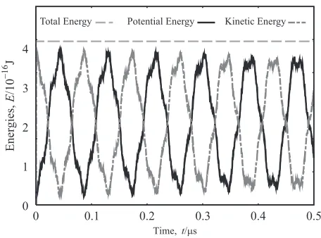
Figure 2 shows that the kinetic and potential energy of the CGPs are oscillating and interchanging alternatively while the total energy is conserved. The period of main oscillation is about 90 [ns]. Figure 3 shows deformation and stress distribution within the rod. The diagonal elements of the stress tensorxx andyy represent local stretch or

compres-sion, while off diagonal components are the shear stresses. It is seen that stretch and compression in y-direction are strongest near the surface in the lower half of the rod. The results are qualitatively reasonable. A more quantitative comparison of the CGP method in 3-dimensions was made

Ny

Nx

Px

Fig. 1 An elastic rod of the CGPs is fixed on the wall and initially the momentumPx¼105is given to all the CGPs at position higher than 8th

layer.

for the elastic constants. Using the Lennard-Jones potential, we computed the elastic constantsC11,C44, andC12with the

coarse grained ratio ¼1024. When compared with those

computed in terms of the MD computation, the relative error of those constants were found to be within 5, 20 and 10%, respectively, in both 2 and 3 dimensions.

3. Lattice Boltzmann Method

Motion of an incompressible fluid is assumed to be described by the lattice Boltzmann method (LBM), which has recently been developed and found to be very effective for computation of the various complex fluid motion. Advantage of the LBM over the conventional fluid mechanics is that (1) the computational algorithm is so simple that actual implementation on the computer is easy, (2) all of the operation is local in physical space so that parallelization of computation is very efficient.8,9)

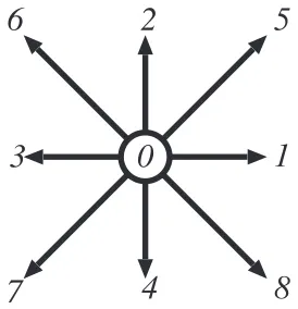
In the LBM, the degrees of freedom of the fluid are represented by ensemble of fluid particles which are assumed to exist only on grid points and allowed to move along

the lines with small number of discrete directions ¼

0;1; ;N and travel to the next grid point in a unit time tLB with prescribed velocity c (see Fig. 4).8,9) In what

follows the length and velocity are nondimensionalized in terms of the grid spacing ~xxLB and the velocity cc~, so that

~

c

ctt~LB¼xx~LB.

Let fðx;tÞ be a distribution function for fluid particles

traveling in the -th direction. Then the density and

momentum are given by

ðx;tÞ ¼X

N

¼0

fðx;tÞ; ð6Þ

ðx;tÞvðx;tÞ ¼X

N

¼0

cfðx;tÞ: ð7Þ

The distribution function with q directions in d spatial

dimensions is referred to as dDqV model. In this study we chose 2D9V model. The evolution of the distribution function is given by

fðxþctLB;tþtLBÞ fðx;tÞ ¼ ½fðx;tÞ

¼ 1

ðfðx;tÞ f

eq

ðx;tÞÞ; ð8Þ

where the left hand side describes the translation and is the collision operator and the so-called BGK

(Bhatnagar-Gross-Krook10)_{) approximation from the Boltzmann kinetics is}

introduced in the second line.is a relaxation parameter and

feq is the local thermal equilibrium distribution function given by

feq¼E 1þ3cvþ

9

2ðcvÞ

23

2vv

; ð9Þ

E0¼

4

9; E¼ 1

9 for ¼1;2;3;4;

E¼

1

36 for¼5;6;7;8 ð10Þ

for 2D9V model which is obtained by expanding the Maxwell Boltzmann distribution function up to the second

order in the fluid velocity. The relaxation parameter is

related to the kinetic viscosity of the fluid as

¼1

3

1 2

: ð11Þ

The equation of motion of the fluid, i.e. the Navier-Stokes equation, can be derived by using the Chapman Enskog expansion, and the reader may consult the references for the detail.8,9) _{It is well known that the spatial accuracy of the}

LBM is the second order in the grid size.

4. Immersed Boundary Method

The macroscopic boundary condition for the fluid phase is assumed to be vðxB;tÞ ¼UB on the boundary whereUB is

the velocity vector of the boundary, and is mesoscopically implemented by imposing the conditions on the distribution function as

fðxB;tþtLBÞ ¼ fðxB;tÞ 2E

cUB

c2

s

; ð12Þ

whereis an index satisfyingc¼ c andEis given by

(10) andcsis the sound velocityc2s ¼c2=3for 2D9V model.

When UB¼0, the above equation means the bounce back

of fluid particle on the rest wall.

When boundary shape of a body is of complex geometry and changes in time, implementation of the above boundary condition and momentum exchange are made in terms of the immersed boundary method (IBM) in this study.11–13)In the IBM, the solid body is regarded as an object which has a distributed force density on its surface so as to match the -200

-150 -100 -50

0 50 100 150 200

σ

σ

σ

σ

Fig. 3 Stress distribution map inside the rod att¼24:0[ns].

2

6

5

1

8

4

7

3

0

boundary condition at the body surface. Suppose that the solid surface is described by points which are smoothly

connected each other. Let Xl be a position of the surface

point which is not necessarily on the fluid grid point (see Fig. 5). Then fðXl;tÞis computed from fat the fluid grid

points by using the Lagrangian interpolation

fðXl;tÞ ¼

X

i;j

ðXl;rijÞfðrij;tÞ; ð13Þ

where is the Lagrangian interpolation function andrij is

the position vector of the fluid grid point nearXl.

Assuming that the fluid particles undergo the elastic collision at the solid surface and the density of the body is much larger than that of the fluid particles, we apply the boundary condition (12) atXl. The change of the distribution

function atXlattþtLBis given by

fðXl;tþtLBÞ ¼ fðXl;tþtLBÞ fðXl;tÞ: ð14Þ

Then the momentum change that fluid receives is

gðXl;tþtLBÞ ¼

X

cfðXl;tþtLBÞsl; ð15Þ

where sl is the surface element. The force acting on the

surface is given by g. Since the force density gðXl;tÞ is distributed on the body surface according to eq. (15), the force must be redistributed on the fluid grid points by the linear rule

gðrij;tþtLBÞ

¼X

l

cfðXl;tþtLBÞDijðrijXlÞsl; ð16Þ

whereDijis

DijðrijXlÞ ¼

1

h2h

xijXl

h

h

yijYl

h

; ð17Þ

hðaÞ ¼ 1

4 1þcos a

2

jaj 2

0 otherwise

8 <

: ð18Þ

in 2-dimensions andhis the grid spacing.

When the external force is applied to the fluid, its effect is to appear as change of the velocity of the fluid as

vðx;tþtLBÞ ¼vðx;tÞ þ

tLBF

ð19Þ

which appears in the velocity field in feq

.

In order to examine the accuracy of LBM for fluid motion and IBM for boundary condition, we applied the methods to 2-dimensional flow around a fixed circular cylinder, computed the drag and lift force acting on it, and compared with the results obtained by the finite difference method

(FDM).14)The Reynolds numberRe¼UD=is 20 and 40,

whereis the kinematic viscosity of the fluid,D¼20is the diameter of the cylinder, andU¼0:1. The drag forceFxand

lift force Fy acting on the cylinder are nondimensionalized

and expressed as the drag and lift coefficients:

CD¼

Fx

ðU2_DÞ=2; CL¼

Fy

ðU2_DÞ=2:

Table 1 shows comparison ofCDcomputed by the present

method with that of the FDM. The values of CD by the

present method tend to be larger around 5% than those of the FDM. One reason for the difference is due to the use of the smoothed kernel function Dij which effectively results in a

hydrodynamic radius slightly larger than the actual radius of the cylinder. It is interesting to note xLB=D0:05,

meaning an increase of 5% in the Reynolds number and a slightly smaller value ofCD, closer to the experimental value.

We would expect that when tends to zero the difference

vanishes. As forCLit is well known that no lift force acts on

the cylinder at these Reynolds numbers, because the flow past cylinder is symmetric about the horizontal line through the cylinder center.

Next we consider two cases at Reynolds number 100; one

is a cylinder fixed in a steady uniform flowU(Case A) and

the other is a moving cylinder with the constant velocityU

in a quiescent flow (Case B). Both cases are physically identical to each other through the Galilean transformation, but the latter is computationally more difficult and is suitable to assess the validity of LBM and IBM. It was found thatCD

was about 1.86 for both cases, which is consistent with the

experimental value. The CL oscillates in time at this

Reynolds number, reflecting the alternative vortex shedding from the cylinder surface (Ka´rma´n’s vortex shedding). The nondimensionalized frequency of the oscillationSt¼fD=U

(Strouhal number), where f is the oscillation frequency,

was found to be about 0.2, again in agreement with the experimental value 0.21. These observations encourage us to use LBM and IBM to study the interaction between solid and fluid from microscopic view point.

5. Coupling between Fluid and Solid

5.1 Characteristic length, time and force in LBM and CGP dynamics

When the fluid motion computed by the LBM and the

Fig. 5 Eulerian fluid grid points for the LBM and Lagrangian points for the solid body in the IBM.

Table 1 Comparison of the drag coefficient (CD).

Re Finite Difference Present Relative error (%)

20 2.045 2.139 4.5

motion of the solid computed by the CGP method are independent of each other, they are numerically integrated in their own length and time scales. However, when they inter-act each other through exchange of momenta at the interface, a physically relevant treatment of the momentum exchange with a mediation of the large gap in space and time scales between the two phases is indispensable. In order to argue those length and time scales, here we consider those quan-tities in the dimensional form which are expressed with (~).

Consider first the fluid motion. In the LBM, the character-istic length and velocity are usually taken to be grid distance xx~LB and the velocitycc~¼

ffiffiffi 3 p

~

c

csfor 2D9V model. Then the

characteristic time is

tt~LB¼ ~xxLB

ffiffiffi 3 p ~ c cs

: ð20Þ

In order eq. (20) to be meaningful, either ~ttLB or xx~LB

must be related to the actual length or time under the consideration. This is achieved by matchingxx~LBto the grid

distance between two adjacent CGPs at the solid surface. Now consider the solid body. The length and time scale of the CG particles are estimated from those of the atoms. Rememberxx~CG¼xx~MD, whereis the coarse graining

factor in one spatial direction. Then characteristic frequency of the CGP can be estimated as!!~CG ffiffiffiffiffiffiffiffiffiffiffiffiffiffiffiffiffiffiffiffiffikKk=kMk

p

where k kdenotes the norm. SincekMk /d andkKk /d2_,

where d is the space dimension, so that !!~CG /1.

Therefore the time increment used in the CGP dynamics can easily be estimated as

tt~CG tt~MD/; ð21Þ

where~ttMDis the time increment used in the MD. The time

scale ratio between the atoms and the CGPs is independent of

the spatial dimensiondand scales asin the same way as

the length. This is a very important result in the numerical matching between the two dynamics.

Now we require the following conditions

~xxLB ¼AL~xxCG; ð22Þ

tt~LB¼ATtt~CG; ð23Þ

for the numerical computation, where AL and AT are the

scaling factors of the space and time increment, respective-ly. The larger AL is, the smoother the solid boundary is. In

other words, the coarse graining factor in the CGP must

be chosen so as for xx~CG to be comparable to xx~LB. We

have chosen a value within the range of 0:8AL1. By

eq. (22), the length scalexx~LB in the LBM is fixed by that

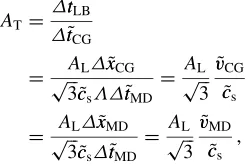
of the CG grid distance. The ratioAT is given by

AT ¼

~ttLB

tt~CG

¼ ffiffiffiALxx~CG 3 p

~

c

cstt~MD

¼ ALffiffiffi 3 p vv~CG

~

c cs

ð24Þ

¼ AffiffiffiLxx~MD 3 p

~

c cstt~MD

¼ ALffiffiffi 3 p vv~MD

~

c cs

; ð25Þ

where we usedxx~CG¼~xxMDandvv~MD¼xx~MD=tt~MD.AT

is governed by the ratio of the characteristic velocity of the oscillation of the atom around the equilibrium position to the

sound speed in the fluid. Typical values used in the MD are ~ttMD¼100tAU¼2:41015[s] for the time step width, xx~MD¼1:91010[m] for the argon atom and vv~MD¼ 0:79105_[ms1_{], while for the aircc~}

s¼3:3102[ms1],

we obtain the ratio as

AT138AL: ð26Þ

SinceAL¼Oð1Þ, the time scale ratio is about a hundred and

that the CGP dynamics part must be integrated about AT

times per one LBM cycle.

In the fluid domain, the characteristic force in the LBM unit is

FLB¼

0cc~ðxx~LBÞd ~ttLB

¼0cc~2ð~xxLBÞd1

¼n0mLB

ffiffiffi 3 p ~ c cs 2

ð~xxLBÞd1; ð27Þ

where0is the fluid density,n0 the number density of fluid molecule andmLBthe mass of fluid molecule. Then the ratio

ofFLB to the Hartree force unitFCG is given by

BF¼

FLB

FCG

¼n0mLB ffiffiffi 3 p ~ c cs 2

ðxx~LBÞd1

mAU _l AU tAU 2 ₁ lAU

¼n0

mLB

mAU

pffiffiffi₃

~ c cs uAU !2 lAU

xx~LB

ð~xxLBÞd: ð28Þ

Typical values for the air are mLB¼4:8511026[kg],

n0¼2:6871019[cmd], so that forAL¼1we have

BF¼0:1963: ð29Þ

The CGP velocity in the atomic unit is transformed to the one in the LB unit by

vLB¼BVvCG; BV¼

uAU ffiffiffi 3 p ~ c cs

ð30Þ

andBV3:85103for the air.

5.2 Coupling

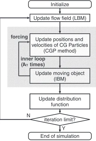
Figure 6 shows the flow chart of the numerical

computa-tion. The CGP process must be iterated AT times for one

LBM cycle. The boundary condition is given by eq. (12) evaluated at thekth CGP positionXk on the solid surface as

fðXkðsÞ;tþtLBÞ

¼ fðXkðsÞ;tÞ 2E

BVcVk

c2

s

; ð31Þ

wheresis a time withint<s<tþtLB andVkis thekth

CGP velocity in the atomic unit. However, since the CGP dynamics is advancedATtimes per one LBM cycle, it is also

necessary to introduce a process of coarse graining of the CGP dynamics in the time domain.

A straightforward way is to assume that the kth CGP on

the surface has the averaged position and velocity

XkðtÞ ¼

1 tLB

ZtþtLB

t

XkðsÞds; ð32Þ

UkðtÞ ¼

1 tLB

ZtþtLB

t

during the integration of the CGPs. However, this leads to the instability of the CGP dynamics because the momentum exchange between the CGPs and the fluid is not conserved at each time step of the CGP dynamics. In other words, this is equivalent to bring the slow variables into the degrees of freedom with the smaller time scale. Rather, the coarse grained variables should appear in the slower variables, the fluid motion, which is done as follows.

At each time step of the CGP dynamics, the distribution

function at the kth CGP position on the surface is

com-puted as

fðXkðsÞ;sÞ ¼X

i;j

ðXkðsÞ;rijÞfðrij;tÞ; ð34Þ

fðXkðsÞ;sþtCGÞ

¼ fðXkðsÞ;sÞ 2E

BVcVkðsÞ

c2

s

ð35Þ

for tstþtLB. Note that the time argument of the

distribution function in the right hand side of eq. (34) is t. It is important also to note that the distribution functions

fðXkðsÞ;sÞ and fðXkðsÞ;sþtCGÞ are those evaluated as

if they were computed at each time step of the LBM cycle. Therefore the change in the distribution function per one CGP cycle is1=AT times the difference, and given by

fðXkðsÞ;sþtCGÞ

¼ 1

AT

fðXkðsÞ;sþtCGÞ fðXkðsÞ;sÞ ð36Þ

and thus the force acting on the kth CG particle on the

surface per one CG cycle is computed as

g_CGðXkðsÞ;sþtCGÞ

¼ BF

X

cfðXkðsÞ;sþtCGÞsk: ð37Þ

On the other hand, the reaction to the fluid is given by

g_LB¼ g_CGðXkðsÞ;sþtCGÞ, so that the corresponding

change in the distribution function at the fluid grid point

rijper one CG cycle becomes

fðrij;sþtCGÞ

¼X

k

fðXk;sþtCGÞDijðrijXkÞsk: ð38Þ

The change in the distribution function per one LBM cycle is given by integrating the above change over the time duration oftLB as

fðrij;tþtLBÞ ¼

ZtþtLB

t

fðrij;sÞds ð39Þ

which is added to fðrij;tþtLBÞas the interaction effects

after the usual LBM process.

The momentum exchange between the fluid and the CGP is done as if the fluid responded to each step of the CGP dynamics. And then the force acting on the fluid is accumulated over the time duration of one LBM cycle. In other words, the dynamics of the fast variables is exactly solved and statistically projected on the slow variables through the time integration of the fast variables. It follows that the above procedure conserves the momentum at the boundary at each time step of the CGP dynamics.

6. Numerical Simulation of Fluid-Solid Interaction

6.1 An elastic rod in 2-dimensional Poiseuille flow

We consider first numerical simulation of an elastic rod in the Poiseuille flow in 2-dimensions. An incompressible viscous fluid flows between two parallel flat plates and the elastic rod composed of the CGPs is fixed on the bottom plate (see Fig. 7). The origin is at the left corner of the bottom plate andx-axis is taken along the bottom plate and

y-axis in the direction perpendicular to the plates. When

uniform pressure gradient in the positive x-direction is

applied to the fluid, the resulting velocity field in the absence of the rod is parallel to the plates and the horizontal

velocity is a quadratic function of y with the maximum

speed on the center line (Poiseuille flow).15)

The number of fluid grid points areL¼600andH¼200

inxandydirections, respectively. The boundary condition of the fluid velocity is v¼ ðvx;vyÞ ¼0 on the plates,

ð4Vmyð1yÞ;0Þ at the inlet, and @vi=@x¼0 for i¼x;y at

the right boundary. On the rod surface vfluid¼Urod is

required. The maximum velocityVmis given byVm¼0:1or

determined from the Reynolds number which is described below. The rod is fixed at 100 units downstream from the

origin, and is composed of NxNy¼1050 CGPs in x

Update distribution function Initialize

Update flow field (LBM)

iteration limit?

End of simulation

inner loop (AT times) forcing

Y N

Update moving object (IBM) Update positions and velocities of CG Particles

(CGP method)

Fig. 6 Flow chart of the numerical computation.

y

x

L

H

Nx

Ny

andydirections, respectively. Again the CGPs are generated from the argon atoms with the spatial coarse graining ratio ¼1024.

We choose as AL ¼1 and AT ¼100. The Reynolds

numbers is defined by R¼VmNy=, which is a

nondimen-sional flow parameter representing the ratio of the convection to the viscous effect, and chosen asR¼25and 250. For the

present level of coarse graining ¼1024, typical values

with dimensions are Ly¼Ny~xxLB ¼17[mm] and air¼ 1:5105[m2s1], so thatR¼25impliesVm¼22[ms1]

which is unrealistically large. Instead, if we chooseVmmuch

smaller value, then the degree of the coarse graining must be increased unrealistically. The above choice of the Reynolds number is very hard for the numerical computation, but here our purpose is to examine whether our computational scheme works even in such tough condition. For more realistic range of parameters, we describes it later on.

The time variation of the x component of the

displace-ment of the CGP at the top left corner of the rod is shown

for R¼25 and R¼250 in Fig. 8, in which the

displace-mentxis in the grid unit and the time is normalized in terms of the wash out time L=Vm as t¼ ðVm=LÞNLBt tLB, where

N_LBt is the number of time steps in the LBM. For R¼25, the variation decays in time, but the oscillation period is almost constant and about 0.45 (81 [ns]) which is very close to the period of 0.50 (90 [ns]) for the eigen mode of the rod alone as we have seen in Sec. 2. This means

that in the initial phase the rod undergoes the impact from the fluid motion and oscillates nearly with its eigen frequency and the motion decays at latter time due to the fluid drag, so that the flow becomes steady and thus the interaction is static at large time. On the other hand, when

R¼250, the motion of the rod does not decay in time and oscillates chaotically although the eigen mode remains predominant. The interaction between the fluid and solid is strong and unpredictable.

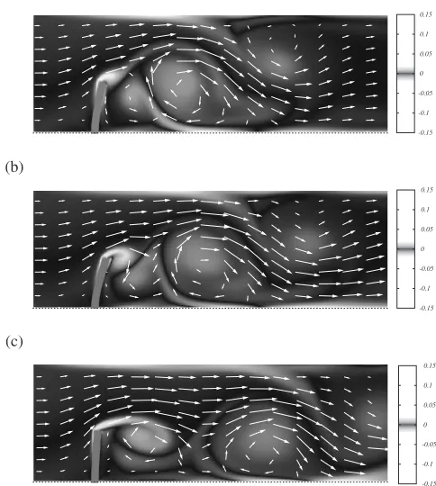
Figure 9 shows the velocity vector and vorticity

distribu-tion for R¼250 at the nondimensional time t¼0:83;

1:00;1:25, respectively. At t¼1:00 a strong negative vorticity is generated near the top left corner of the rod

which is bent due to the fluid motion, and at t¼1:08 the

eddy is about to be shed into the fluid while the bending of the rod becomes almost maximum. When the eddy is separated and convected downstream, the rod returns to be straight, and similar motion continues. Correspondingly, when the bending of the rod becomes maximum the stretch (compression) of the lower left (right) corner of the rod iny

direction becomes maximum (figures not shown).

6.2 Flow induced by a collective motion of an array of elastic rods

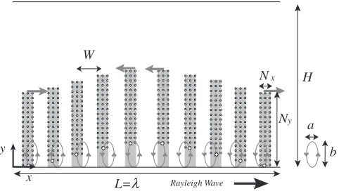
We now consider more realistic problem of fluid transfer by a kind of MEMS (NEMS) (Micro(Nano)-Electro-Mechanical System) device. It has been known that an elastic surface wave (Rayleigh wave) can convey a body in a direction opposite to the traveling wave. It is very interesting and useful for the future development of micro(or nano) scale fluid devices to examine whether the fluid can be transferred by using similar technique.

(a)

(b)

Fig. 8 Variation of thexcomponent of the displacement of the CGP at top left corner of the plate.R¼25(a) and 250 (b). The displacementxis in the grid unit and the time is normalized in terms of the wash out timeL=Vmas t¼ ðVm=LÞNLBt tLB.

-0.15 -0.1 -0.05 0 0.05 0.1 0.15

(a)

-0.15 -0.1 -0.05 0 0.05 0.1 0.15

(b)

-0.15 -0.1 -0.05

0 0.05 0.1 0.15

(c)

Consider an array of elastic rods which are fixed on the horizontal plate above which an incompressible fluid fills the space. We assume that the Rayleigh wave is traveling on the surface in the positive xdirection and the array of the elastic rods undergoes a collective motion in response to the Rayleigh wave (see Fig. 10). With this set up we consider how the fluid motion is induced and how much amount of the fluid is transferred. The number of the fluid grids is 500 (Case A) or 1000 (Case B) in the horizontal direction and 100 in the vertical direction, respectively, and the boundary conditions for the fluid is the periodic condition at x¼0 and L, while v¼Urods on the rods, and the slip condition

(the tangential viscous stress is zero) is applied aty¼Hin order to mimic the free surface of the fluid. Each rod is the same as that used in the previous section, and 10 rods are

placed with separation distance W ¼50xLB for Case A

and W ¼100xLB for Case B. In order to examine the

effect of the microscopic elastic matrix of the rod on the

fluid-solid interaction, we have changed C of eq. (1) by

multiplying a factor ¼1:0;0:5;0:2for which computation is referred to as Run I, Run II, and Run III. This change leads to the variation of the macro scopic stiffness of the rod and the characteristic magnitude is, for example,CCG

11

21;10:5;4:2[GPa]. The ratios AL and AT are 1 and 100,

respectively.

We assume that instead of solving the equation of the Rayleigh wave the motion of the horizontal plate due to the Rayleigh wave propagation is kinematically described as

x¼x

a

2sinðkx!tÞ; y¼

b

2cosðkx!tÞ; ð40Þ

for the position vector ðx; yÞof the surface element of the

horizontal plate, wherekand!are the wavenumber and the

angular frequency of the Rayleigh wave. The amplitudesa

and b are linearly dependent each other and fixed by the

Poisson ratio of the bottom plate, but here we take the ratio

a=b to be an arbitrary parameter. The wavelength of the

Rayleigh wave is assumed to be500xLB(¼100[mm]) and

its amplitude is a¼0:5xLB (¼100[nm]) and b¼xLB

(¼200[nm]) in x and y directions, respectively. The

frequency ff~of the Rayleigh wave is chosen to be 1 [MHz] so that the typical velocity of the oscillation of a point

on the horizontal bottom plate is about URay¼!Raya

(0:6[ms1_{]). The Reynolds number is chosen to be}

R¼URayNy=¼0:15 with Ny¼50 which is the height

of the rod.

Figure 11 shows the velocity and vorticity distributions at the nondimensional time tt~ff~¼32:3 for the Runs I and III withW¼50xLB (Case A), whereTT~¼1=ff~is the time for

the Rayleigh wave to travel the fundamental domainL. The vorticity concentrates near the tops of the rods. It is also found that the spatial coherency of the vorticity distribution for Run III prevails over the region wider than that for Run I. Figure 12 compares the evolution of the time accumulated total volume flux (in the LBM unit) defined byQðxÞ ¼R₀tR₀Hvxðx;y;sÞdydsatx¼0for the Cases A and

B. The curve for ‘‘Rigid’’ is the results of the rigid rod in which the grid spacing of the CGP is fixed. The average horizontal velocity in the dimensional form is given by

~

V V V

V ccQ~ =ðHtÞand found to be about 9 [mms1] for Run III

of Case A and about 7 [mms1_{] for Run III of Case B,}

respectively. It follows that general trend is (1) the fluid is transferred in the opposite direction to the Rayleigh wave, (2) the fluid transfer is enhanced by softer (smaller stiffness) and thicker rods, which resembles the flagellum.

Instead of using the elastic rod array, we have also studied the case of a continuous layer of the CGPs over the horizontal plate and the Rayleigh wave travels within the layer. The thicker the layer of the CGPs becomes, the more the fluid is transferred in the opposite direction to the Rayleigh wave, although the time accumulated total volume fluxQis smaller than in the case of the rod array. The average horizontal velocity is about 3 [mms1] for the case of layer of 10 CGPs. Therefore it is suggested that in order to transfer the fluid by using the Rayleigh wave a flagella like structure is more effective.

7. Summary and Conclusions

We have studied the interaction between the fluid and the elastic body from the mesoscopic view point for the fluid and the microscopic view point for the solid. The CGP system was constructed from the atoms by using the RCGP method under the assumption of the local thermal equi-librium and the phonon approximation, and the system was integrated in the same way as in the MD but with different time step width. As for the fluid motion the LBM method was used. In the LBM, the distribution function of the ensemble of fluid particles is introduced and evolved according to the shift and collision processes, thus the approach is mesoscopic. Any specific character of the fluid molecules and of the length and time scales do not enter the LBM dynamics, and the fluid motion emerges as collective motion in the long wavelength limit.

Both dynamics are coupled through the momentum exchange on the surface of the solid body, where the length and time scales in the LBM are fixed. The important point is that the coarse graining process should be made not only in constructing the CGP system but also in this momentum exchange process where two physical processes with widely different spatial and time scales meet at the small spatial domain. The coarse grained quantities obtained by the statistical averaging of the fast variables should appear only in the dynamics of the slow variables.

Rayleigh Wave

x y

W

N x H

Ny _a

b

L=

Our method was applied to the cases of single or multiple elastic rods which are composed of the CGPs in the two dimensional Poiseuille flow. It was found that the method was successful and useful to describe the interaction between

fluid and solid with scale disparity. The results presented in this study are, however, qualitative rather than quantitative because our computation was limited to 2-dimensions and some parameters were not those of the actual system. Further quantitative verification is necessary for the future development, which includes quantitative comparison of the oscillation period, of the solid body, drag and lift acting on it, and so on, and 3-dimensional computation is very important. These are challenges to the computation for the multiscale physics, and the work is in progress and will be reported somewhere.

Acknowledgments

The authors thank the Information Technology Center of Nagoya University for his providing computational support.

REFERENCES

1) C. M. Ho and Y. C. Tai: Ann. Rev. Fluid Mech.30(1998) 579. 2) R. E. Rudd and J. Q. Broughton: Phys. Rev. B58(1998) 5893. 3) R. E. Rudd and J. Q. Broughton: Phys. Rev. B72(2005) No. 144104. 4) S. Ogata, E. Lidorikis, F. Shimojo, A. Nakano, P. Vashishta and R. K.

Kalia: Comput. Phys. Commun.138(2001) 143.

5) S. Ogata, F. Shimojo, R. K. Kalia, A. Nakano and P. Vashishta: Comput. Phys. Commun.149(2002) 30.

6) R. Kobayashi, S. Ogata, Y. Inoue, J. Tanaka and T. Gotoh: Proc. APCOM07 in conjunction with EPMESC XI, MS9-1-3. December 3–6, 2007, Kyoto, JAPAN.

7) R. Kobayashi, T. Nakamura and S. Ogata: Mater. Trans.49(2008) doi: 10.2320/matertrans.MB200813.

8) S. Chen and G. D. Doolen: Ann. Rev. Fluid Mech.30(1998) 329. 9) S. Succi:The Lattice Boltzmann Equation for Fluid Dynamics and

Beyond, (Oxford University Press, 2001).

10) P. Bhatnagar, E. Gross and M. Krook: Phys. Rev.94(1954) 511. 11) C. S. Peskin: J. Compu. Phys.25(1977) 220.

12) Z. G. Feng and E. E. Michaelides: J. Compu. Phys.195(2004) 602. 13) X. D. Niu, C. Shu, Y. T. Chew and Y. Peng: Phys. Lett. A354(2006)

173.

14) S. C. R. Dennis and J. G. Z. Chang: J. Fluid Mech.42(1970) 471. 15) G. K. Batchelor:An introduction to Fluid Dynamics, (Cambridge Univ.

Press, 1967).

(a)

(b)

−150 −100 −50 0

0 2 4 6 8 10

V

olume Flux,

Q

x=0

Timesteps, t/104 Rigid

Run I Run II Run III

−150 −100 −50 0

0 2 4 6 8 10

Volume Flux,

Q

x=0

Timesteps, t/10 Rigid

Run I Run II Run III

4

Fig. 12 Comparison of the time accumulated total volume fluxQx¼0 at

x¼0 for three values of the stiffness, Runs I, II, and III Case A: W¼50xLB(a) and Case B:W¼100xLB(b).

(a)

(b)

-0.0006 -0.0004 -0.0002

0 0.0002 0.0004 0.0006

-0.0006 -0.0004 -0.0002

0 0.0002 0.0004 0.0006