A new, robust, and generic method for the quick creation of smooth paths and near time optimal path tracking

(1)

NEAR TIME-OPTIMAL PATH TRACKING

Matthew Bott

A Thesis Submitted for the Degree of PhD

at the

University of St. Andrews

2011

Full metadata for this item is available in

Research@StAndrews:FullText

at:

http://research-repository.st-andrews.ac.uk/

Please use this identifier to cite or link to this item:

http://hdl.handle.net/10023/2095

This item is protected by original copyright

(2)

A new, robust, and generic method for

the quick creation of smooth paths and

near time-optimal path tracking

Matthew Bott

School of Computer Science

University of St Andrews

(3)

Abstract

Robotics has been the subject of academic study from as early as 1948. For much of this time, study has focused on very specific applications in very well controlled environments. For example, the first commercial robots (1961) were introduced in order to improve the efficiency of production lines. The tasks undertaken by these robots were simple, and all that was required of a control algorithm was speed, repetitiveness and reliability in these environments.

Now however, robots are being used to move around autonomously in increasingly unpredictable environments, and the need for robotic control algorithms that can successfully react to such conditions is ever increasing. In addition to this there is an ever-increasing array of robots available, the control algorithms for which are often incompatible. This can result in extensive redesign and large sections of code being re-written for use on different architectures.

The thesis presented here is that a new generic approach can be created that provides robust high quality smooth paths and time-optimal path tracking to substantially increase applicability and efficiency of autonomous motion plans.

The control system developed to support this thesis is capable of producing high quality smooth paths, and following these paths to a high level of accuracy in a robust and near time-optimal manner. The system can control a variety of robots in environments that contain 2D obstacles of various shapes and sizes. The system is also resilient to sensor error, spatial drift, and wheel-slip.

In achieving the above, this system provides previously unavailable functionality by generically creating and tracking high quality paths so that only minor and clear adjustments are required between different robots and also be being capable of operating in environments that contain high levels of perturbation.

The system is comprised of five separate novel component algorithms in order to cater for five different motion challenges facing modern robots. Each algorithm provides guaranteed functionality that has previously been unavailable in respect to its challenges. The challenges are: high quality smooth movement to reach n-dimensional goals in regions without obstacles, the navigation of 2D obstacles with guaranteed completeness, high quality smooth movement for ground robots carrying out 2D obstacle navigation, near time-optimal path tracking, and finally, effective wheel-slip detection and compensation. In meeting these challenges the algorithms have tackled adherence to non-holonomic constraints, applicability to a wide range of robots and tasks, fast real-time creation of paths and controls, sensor error compensation, and compensation for perturbation.

This thesis presents each of the above algorithms individually. It is shown that existing methods are unable to produce the results provided by this thesis, before detailing the operation of each algorithm. The methodology employed is varied in accordance with each of the five core challenges. However, a common element of methodology throughout the thesis is that of gradient descent within a new type of potential field, which is dynamic and capable of the simultaneous creation of high-quality paths and the controls required to execute them. By relating global to local considerations through subgoals, this methodology (combined with other elements) is shown to be fully capable of achieving the aims of the thesis.

(4)

Acknowledgements

I thank EPSRC and the University of St Andrews for providing funding without which I would not have been able to conduct my work. Thanks also go to my supervisor Michael Weir for guiding me in becoming a scientist from my origins as an engineer. Finally I thank Jon Lewis for his assistance in my first year.

I thank my examiners John Hallam and Kevin Hammond for taking the time to both read my thesis and perform the viva.

On a more personal note, I also thank the office mates I’ve had, Peter, Natalie, & later on Lakshitha you’ve helped me a lot over the years with lots of laughs, procrastination a plenty, and the odd rant here and there. Thanks also go to the many friends I’ve made during my time in St Andrews without whom I wouldn’t have made it through. Finally my parents, for the support and patience they’ve shown all along, especially in my final year(s).

Finally I’d like to give thanks to the internet, part of which has gifted me with this quote which I think sums up the creative side of a PhD.

“I didn’t just look over and see some hippo. I saw where a hippo was not, and said no.

(5)

Declaration

I, Matthew Bott hereby certify that this thesis, which is approximately 80,000 words in length, has been written by me, that it is the record of work carried out by me and that it has not been submitted in any previous application for a higher degree.

I was admitted as a research student in September 2006 and as a candidate for the degree of Doctor of Philosophy in May, 2007; the higher study for which this is a record was carried out in the University of St Andrews between 2006 and 2011.

Date signature of candidate

I hereby certify that the candidate has fulfilled the conditions of the Resolution and Regulations appropriate for the degree of Doctor of Philosophy in the University of St Andrews and that the candidate is qualified to submit this thesis in application for that degree.

Date signature of supervisor

In submitting this thesis to the University of St Andrews I understand that I am giving permission for it to be made available for use in accordance with the regulations of the University Library for the time being in force, subject to any copyright vested in the work not being affected thereby. I also understand that the title and the abstract will be published, and that a copy of the work may be made and supplied to any bona fide library or research worker, that my thesis will be electronically accessible for personal or research use unless exempt by award of an embargo as requested below, and that the library has the right to migrate my thesis into new electronic forms as required to ensure continued access to the thesis. I have obtained any third-party copyright permissions that may be required in order to allow such access and migration, or have requested the appropriate embargo below.

The following is an agreed request by candidate and supervisor regarding the electronic publication of this thesis:

Access to printed copy and electronic publication of thesis through the University of St Andrews.

Date signature of candidate

(6)

Chapter 1 – Introduction

1.1 Chapter Overview

This chapter forms an introduction to the thesis. As such, it will first introduce the motivation for the thesis followed by its objectives. Next the contribution provided by achieving the outlined objectives is described. The penultimate section outlines the structure of the thesis, and finally the publications produced during the thesis are given.

1.2 Motivation

Autonomous mobile robots are being used with increased frequency in more and more areas. Examples include unmanned aircraft and bomb disposal robots used by the military to reduce risk to personnel, automated vacuum cleaners to reduce workload in the home, and planetary rovers for exploring mars. This increase in the use of mobile robots is only possible due to the research conducted in the field of autonomous mobile robotics. The work detailed in this thesis aims to further this research in order to expand on the existing capabilities of autonomous robots.

Whilst the examples of military robots, household cleaner drones, and planetary rovers may seem very different, one element that they all have in common is the need for a robust navigation algorithm. In fact, robust navigation is an aspect that is common to all mobile robots used outside of well-defined environments. An algorithm that acts in an environment that is not well known must be robust in order to cope with any unpredictable changes that may be present.

In addition to the ability to robustly navigate between locations, the ability to move in a given manner is also useful. A manner of movement that is desirable for a wide range of robots is the ability to move smoothly. This desirability is because smooth movement allows greater conservation of momentum, which is to say that it requires less energy to change the direction in which a robot is moving by a small amount than a large amount. Therefore conserving momentum allows the conservation of energy. Smooth paths can also allow an increase in the speed at which a robot may travel as a robot has to slow down in order to achieve tight corners more than it does for gentle turns. Smooth movement by its very nature adjusts the direction in which a robot moves gradually and does not contain sharp changes in direction. Undulatory smooth movement in particular has the additional property of not including any changes in direction that are not necessary for a robot to reach its goal location. A common example of an unnecessary direction change is a loop in a path.

In addition to smooth movement it is also desirable to be able to re-plan paths quickly. This desire stems from the unpredictable and changing nature of real world environments and to allow real-time execution of tasks at speed. Examples of unpredictable changes in an environment are the detection of previously unknown obstacles, a change in travel surface conditions (loss of grip), or the development of winds that blow the robot off course. An algorithm that cannot quickly re-plan paths cannot quickly adapt paths to changes in the environment, and may not be able to achieve its given task, hence it is desirable to be able to re-plan paths quickly. Historically one way around this issue has been to bring the robot to a halt, as stopping the robot allows for the time required in planning a new path to account for changes in the environment. However it is clearly more desirable to be able to quickly re-plan a path so that the robot need not come to a halt and can instead continue with its navigation unhindered and at speed.

(14)

may be undertaken in a given time period. A commercial example is that a premium is often paid for services that can achieve a task within a shorter time.

The final desirable quality discussed here for robotic control algorithms is genericity. Genericity here means the applicability of a robot control algorithm to a wide range of robots for a wide range of navigation tasks with minimal changes required to the original algorithm. The desirability of genericity increases with the number of robots that could potentially benefit from the capabilities given by an algorithm. As has been detailed above, the qualities of smoothness, adaptability through quick re-planning, and time optimality are widely applicable to mobile robots in the real world. Therefore, genericity is also desirable in an algorithm that is capable of providing these qualities to enable it to be used as widely as possible.

It is the above desirable qualities that this thesis attempts to embody. The motivation for this thesis is the widely applicable and desirable nature of these qualities in a world where robotics are at the forefront of development and progress in many areas of life. Given this motivation, the following section defines the specific objectives of this thesis.

1.3 Thesis Objectives

Given the motivation for the thesis described in the previous section, the objectives follow in a straightforward manner. The objectives of this thesis are:

1. To provide undulatory smooth, low curvature paths 2. To provide resistance to drift from sources of:

a. Side wind style disturbances b. Sensor errors

c. Errors in control execution d. Wheel-slip

3. To allow navigation of obstacles

4. To provide near time-optimal following of a path

5. To allow quick re-planning of paths (never more than a second)

6. To allow quick response times for the following of paths (never more than 0.05 seconds) 7. To allow application to a wide range of robots and navigation spaces

The times mentioned above relate to running an algorithm encoded in Java 7 on an Intel Core Duo 1.8Ghz machine with 2GB ram (as this is the programming language and machine used throughout this thesis).

The objectives outlined above represent a large challenge, as well as a number of individually desirable components. In order to allow the individual application of these components, five separate algorithms are developed, each of which contribute to the achievement of some of the objectives and when used together meet all of them. Each of these five algorithms represents a contribution to the field of robotics on their own, and is suitable for use with algorithms other than those given here.

1.4 Contributions

This thesis makes contributions to two areas of mobile robotics, these are path planning and path tracking. Path planning concerns the creation of a path to be followed, and path tracking corresponds to following this path.

(15)

been defined previously. Whilst individually available, these qualities have not been found (by the author) to all be present in any one pre-existing algorithm. In addition, the research conducted by this author leads to the conclusion that it would be difficult if not impossible for any existing method to be developed in order to achieve these aims (excepting large increases in computational power). The overall result of these qualities is the ability to smoothly navigate a robot from one state to another in an environment that may contain 2D obstacles, whilst catering for side wind style drift as well as both control execution and sensor errors.

A contribution made to the area of path tracking is the use of lookup tables. These tables enable quick calculation of a near time optimal speed for the robot to travel at accounting for an individual robot’s dynamics. Dynamics here refers to a robot’s acc/deceleration, speed of steering adjustment and speed at which given curvatures may be executed without wheel slip. The algorithm also allows the updating of the calculated speed to maintain feasibility in the face of drift. In addition, the algorithm does not use a torque-based model, and as such requires less data regarding the specific robot in order to function. [A torque-based model requires information regarding the mass of each component within the robot, and how each actuator is linked to each part of the robot, as well as the forces that the actuators are able to exert on these linkages.] It is also seen as advantageous that the developed method is able to calculate both the near time-optimal speed, and the controls required to execute it, removing the need for a separate path tracker (compared to some existing algorithms). Note that the method described here claims only near time-optimality whereas other methods have claimed time-optimality. This is because the method described here deals with unpredictable drift, which (as far as is known) has not been dealt with in existing methods. In the face of this unpredictable drift, it is impossible for any method to retain full time-optimality. This impossibility stems from the fact that drift is likely to move the robot in a sub-optimal way and it is impossible to completely counter an unpredictable direction and magnitude of drift before it occurs.

A contribution made to the movement of ground robots in general is the combination of wheel-slip prediction and reaction to changes in slip resulting from any changes to the travel surface. It is important to note that only basic sensors giving the robot’s location and heading, and the movement of the steering and driving wheels, together with a forward kinematics model are used. [A forward kinematics model predicts the movements of a particular robot given an initial robot state and the controls to be executed.] In addition to this, the algorithm is path independent, which is to say that the algorithm is based solely on the robot itself and the travel surface. This independence contrasts with some existing methods that require knowledge of the whole of the robot’s designated route and therefore cannot be used when there is no designated route. Finally, the algorithm is also capable of calculating drift that has occurred due to non wheel-slip sources, although no recommendations are produced for the avoidance of this drift. The reason that no recommendations are produced is that the course of action taken by existing algorithms is still applicable.

1.5 Thesis Structure

The structure of the thesis is as follows.

Chapter 2 provides background information in mobile robotics and defines the key concepts used.

(16)

Chapter 3 details the development of the first algorithm that provides undulatory smooth, drift resistant travel in generic spaces that do not contain obstacles. Chapter 4 develops an algorithm for 2D (x,y) only navigation, where x denotes east to west travel, and y denotes south to north travel. Chapter 4 provides less smooth travel than that detailed in chapter 3, but allows for obstacles, which may be present in the travel environment and provides a resistance to sensor errors. Finally chapter 5 combines chapters 3&4 to allow navigation of generic spaces, which may contain (x,y) obstacles. The algorithm in chapter 5 represents the best of both chapters 3&4 without their weaknesses.

Chapter 6 details an algorithm that provides near time-optimal tracking of a path. In doing so it accounts for the robot’s acceleration, top speed, and the maximum speed at which a given curvature may be executed. The algorithm also allows the avoidance of wheel slip and its associated drift for a fixed travel surface. Chapter 7 contrasts with chapters 3-6 in that the algorithm detailed does not control a robot but instead provides recommendations of limits in acc/deceleration and maximum speed for a given curvature. Adherence to these (continually updated) limits allows wheel-slip to be avoided if the travel surface is varied, and the amount of friction available in any one environment is subject to change. Combined with chapter 6 chapter 7 would allow for near time-optimal travel on a varying travel surface (although this is not tested here).

Chapter 8 concludes the thesis discussing the achievements made by each algorithm both individually and when combined. This chapter also outlines further work that would allow improvement on the abilities of the algorithms discussed.

1.6 Publications

During the course of producing this thesis two conference papers have been published. These papers relate to chapters 3&5 and references are shown below:

Michael K. Weir, Jon P. Lewis, Matthew Bott: Enabling nonholonomic smoothness generically allowing for unpredictable drift. ICARCV 2008: 2072-2077

(17)

Chapter 2 – Background

2.1 Chapter Overview

This chapter provides background on areas relevant to the thesis as a whole. It is important that the reader understand these concepts before reading the remainder of the thesis. The layout of this section is as follows.

First a brief history of robotics and applications for autonomous robots in the modern world is given to introduce the wide-ranging area of research that is mobile robot navigation.

Secondly a comparison is provided between the two main forms of navigation algorithm, path planning and path tracking. Path planning consists of creating a path for the robot to follow, which may or may not include the creation of controls that allow the robot to follow the created path. Path tracking consists of following a given path, this either consists of creating controls required to follow the given path, or the alteration of pre-existing controls to account for unexpected perturbation.

Thirdly the factors that affect the design of a robotic motion-planning algorithm are given. Examples of these factors include the data available, the criteria for success, and the speed at which the algorithm must complete its task.

Fourth is an introduction to robot kinematics and dynamics. Kinematics and dynamics affect the way in which a robot is modelled, with kinematics forming a simpler model, and dynamics relating to a more complex model. Dynamics covers the more complex dynamic variables aspects of the robots motion such as robot momentum and acceleration as opposed to kinematic variables for example an x,y location.

The fifth item discussed is the holonomic or non-holonomic constraints that a robot may be subject to. In brief, holonomic constraints are positional, for example a physical obstacle, where any paths that do not collide with this obstacle may be taken through the environment. In contrast, non-holonomic constraints are non-positional i.e. act throughout an environment. For example a car-like robot cannot move sideways. Robots that are subject to non-holonomic constraints pose a more complicated control problem than those subject only to holonomic constraints as their movements are more restricted. Non-holonomic constraints are present in every chapter of this thesis and therefore a grasp of the difficulties posed is vital to the understanding of this document.

The sixth topic covered is the definition of smoothness and genericity. These are important concepts for the thesis that are used throughout, but take on different meanings within the research community, and therefore require definition here.

The seventh topic covered is that of drift. Drift is the general name given to any perturbation in the robot’s movements (from those expected). This section will detail the different forms of drift that exist, and identify those which will be tackled over the course of this thesis.

The penultimate topic is an introduction to two popular kinds of control algorithm; these are gradient descent and rapidly exploring random trees (RRT’s). Gradient descent is the basis of all algorithms in this thesis, whilst RRT’s are used as a benchmarking algorithm to show the effectiveness of the methods developed and presented here relative to a popular approach.

(18)

2.2 A Brief History Of Autonomous Robotics

Autonomous robotics refers to the area of research surrounding robots that are capable of autonomous movement, and are capable of executing more than one task. Therefore a vending machine, whilst it contains moving mechanical parts, and is able to perform more than one task does not constitute an autonomous robot. In contrast, a robotic arm does constitute an autonomous robot, as it is able to perform a wide range of tasks and movements without human intervention.

Autonomous robots began (outside of research centres) in 1961 as robot arms [78]; these were programmed by a human operator and used to perform tasks that the human operator was either unable, unwilling or less efficient to perform. Such robots were used in heavily structured environments and for largely repetitive movements such as factory production lines.

The next large step (outside of research centers) was in 1969 and consisted of automated lawnmower robots that were capable of autonomous movement beyond a fixed base [1]. These robots also began to function in environments that were more varied, and unpredictable than those previously seen in factory settings. In order to control these robots, more sophisticated control algorithms were required and thus the mobile robotic control algorithm was born.

The modern control algorithm has two main objectives at heart, the first of these is robot (and if relevant human) safety, this means that the robot must be controlled in a manner that does not cause it to come to harm. Harm may come from a variety of sources such as collision with obstacles, or internal damage due to pushing motors beyond their recommended operational zones. The second is the achievement of a task, (e.g. navigation from one point to another).

2.3 Path Tracking and Path Planning

There are two main forms of navigation algorithm, these are path planning and path tracking. The two forms have their relative strengths and weaknesses and are used in different circumstances depending on which is better suited. This section will introduce the two forms of algorithm, and provide a comparison of the two highlighting the circumstances to which each is suited.

2.3.1 Path Tracking

Path tracking, as the name suggests consists of tracking an established path. Path tracking algorithms assume that the established path is be provided by another algorithm.

The primary aim of a path-tracking algorithm is to track a given path within as given level of accuracy [62]. It is important to note that the level of accuracy within which a path may be tracked will be dependant on the feasibility of the provided path. It should also be noted that whilst a path may be feasible when presented it may become infeasible due to changing environmental conditions. This may mean that it is impossible for the path tracker to re-join the path and arrive at its end.

Secondary aims may include travelling at a desired or optimum speed [109], or minimising energy used [110].

(19)

Path trackers are able to update the controls used in following the path at a high rate (relative to path planners) as they need only produce controls relating to the next section of the path at any one point. This high rate is key in the achievement of path tracking to high levels of precision as it allows new sources of drift to be identified and countered quickly before they are able to affect the path tracking to a large degree.

As robot controls can be updated frequently, and move the robot only a short distance along the path before controls are re-calculated [74], a high degree of flexibility is provided. This flexibility stems from the fact that any one set of controls are applied for a short time only, therefore if a particular linear movement results, then this will only occur for a short time. This flexibility is key in path tracking as a large number of rapidly changing linear moves is able to approximate a path of any shape.

2.3.2 Path Planning

Path planning (as the name suggests) refers to planning a path in configuration space. A path planner may or may not provide the controls required to follow the planned path.

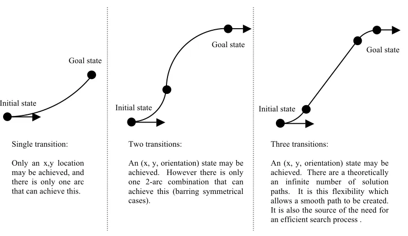
The primary aim of a path planner is to connect two states, these states are usually a set of co-ordinates that define a point in Cartesian space [125], but other variables such as an end orientation [47], speed [44], or curvature [77] may also be included. Secondary aims for path planners regard factors such as the shape [66], length [100], or speed profile [108] of the path connecting the two states.

As a path planner creates an entire path between two states, the fast response time found in path tracking algorithms is not typically present. If used in an environment that is subject to varying levels of perturbation, or contains obstacles the location of which is unknown a-priori then a path planner may be used in a sequence of plan and execute stages [32]. These interleaved stages allow movement to be made, the observation of changes in the known environment, and the re-creation of a plan accounting for these changes. These interleaved plan and execute cycles continue until the destination state is reached.

The number of path segments required to produce a complete plan varies depending on the specific path planner used, and the nature of the path segments used. Some path planners use a combination of a small fixed number of small fixed path segments, these planners require a large number of segments in order to form a path [59]. Other path planners use a small number of variable path segments (in some cases just 1 [77]). Any and all combinations of the above are also possible.

2.3.3 Suitability Comparison (Planning vs. Tracking)

The previous sub sections have outlined the operation of path planners and path trackers, this sub-section provides a comparison of the two, and highlights the different applications for which each is used. Finally a feature table is given to provide a side-by-side summary of the methods.

The key factor in deciding whether a path planner or a path tracker should be used (whilst the robot is in motion) is the level of predictability within the environment. If it is possible that a path that is planned a priori may become infeasible as the robot progresses then a path planner must be used. An example of this is unknown obstacles within the environment, if such obstacles are present, then some degree of path planning will be required in order to construct a path around an obstructive obstacle.

(20)

planner. This is due to the high frequency or control updates that are possible by use of a path tracker. This high frequency of updates allows better following of a planned path than that possible by updating the path to account for perturbation changes at a lower rate as the data used in calculating controls is more accurate.

[image:20.595.131.461.183.294.2]

The relative ability and suitability of path planners and path trackers are given in Table I below.

Table I - Relative Abilities of Path Trackers & Planners Ability/Suitable Environment Path Tracker Path Planner

Rapid control update !

Perturbation resistance ! !

Path quality control !

Path speed control ! !

Single step planning !

Multi step planning ! !

Accommodation of unknown obstacles !

Highly unpredictable rapidly varying amounts of drift !

Path may be rendered impossible to follow !

Dynamic goal location !

In real life scenarios it can sometimes be best to combine path trackers and path planners for example work by Takiguchi and Hallam [105]. Here combining the two allows for all of the strengths of each, a global path planner provides a plan accounting for global issues i.e. obstacles, whilst a path tracker ensures that the created plans are followed to a high degree of accuracy. An extension to this that would further capitalise on the strengths of both is that the global path planner could re-plan if new obstacles are detected, or a new goal location was received.

2.4 Algorithm Design Considerations

When constructing an algorithm for the control of autonomous robots, a variety of factors must be taken into consideration. These factors shape the algorithm and define its acceptable operational limits. The main factors to be considered are:

1. What must the algorithm achieve? I.e. what are the criteria for success

2. What data are available in order to allow the success of the algorithm? I.e. how much information regarding the robot and its environment may be accessed by the algorithm

3. What computational power is available? I.e. must the algorithm limit the amount of memory it uses, or processor speed that it requires to function.

It is often the case that not all of these factors are specified by the task undertaken, however they must all be considered carefully, and stated as assumptions when describing an algorithm to ensure that any potential users are aware of any limitations and requirements.

(21)

2.4.1 Success Criteria

In robotics success criteria are many and varied. However, popular criteria include:

1. Reaching a target location in space [125]. 2. Maintaining a target speed [93].

3. Travelling towards a target in a particular manner, is known as path quality and may include:

a. Minimising distance travelled [100] b. Conserving power consumed [113] c. Smoothing the motions of the robot [66] d. Forwards only motion [73]

4. The avoidance of physical obstacles [32]

5. The adherence to control limits, for instance joint limitations or prescribed minimum turning circles [99]

6. Resistance to sensor errors [97] 7. Resistance to drift [109] 8. Low computational cost [77] 9. Variety of robots controlled [104] 10. Variety of tasks possible [104]

The individual criteria used will relate to the robot to be controlled and the specific task to be undertaken.

As has been mentioned previously (2.1) this thesis is comprised of 5 separate algorithms each with their own criteria for success. However, there are two elements that are common to all, these are speed of control calculation, and applicability. Speed at which controls are calculated is important as algorithms designed here are intended for use in real time and in changing environments; therefore it is crucial that each algorithm be capable of updating its commands in real time if it is to be able to perform its task. Applicability is important because an algorithm that may be used on a wide range of robots is more useful to the community as a whole. To achieve this wide applicability, the algorithms detailed in this thesis are designed in such a manner that robot specific information relied upon is kept to a minimum (that is always available), and controls are produced in a manner that can be applied to any robot.

2.4.2 Available Data

When an algorithm controls a robot, it requires certain information regarding the robot and the environment in which it is placed. Information is also required regarding the task that the algorithm is required to perform. However the amount of information that is available may vary from task to task, robot to robot, and environment to environment. Therefore an algorithm that uses the least amount of and most readily available information has the highest chance of being usable for a randomly chosen robot and environment.

For simplicity, available data is classified here as full or limited, these categories are commented upon below for the environment, robot and task:

Area Full Limited

Environment If full knowledge of the environment is available, the locations of all obstacles are known, as is the available friction at each point, the angle of any slopes, and any wind or other disturbances that may be present. Full knowledge

(22)

extends to any time varying factors such as moving obstacles, or varying wind conditions.

Full environmental knowledge is available in environments as that may be easily controlled.

Using full environmental knowledge an algorithm can safely plan all movements offline and it is also safe to assume that the path created may be followed without interference from the environment [106]. Note that this only holds providing that no unknown variables are introduced by the robot or task.

direction in which an obstacle is moving from a series of snapshots of its location.

Some but not all environmental knowledge is commonly available where aspects of the environment are unspecified and uncontrolled

When limited information is available, the algorithm must be able to react quickly to any new information received and update any planned movements if collisions are to be avoided and the robot is to successfully complete its task.

Robot For full knowledge of a robot the weight and size of every component must be known as well as the interactions between each part. The robot must also be very reliable to ensure that these values hold over time.

Examples where full robot knowledge may be available include moon rovers [29], space satellites, or deep-sea exploration vehicles. These robots are expensive, and the tasks set are also highly specialised. The large expenditure upon the robot allows the creation of a highly specific and custom-made algorithm.

Full knowledge of the robot means that a detailed model may be created, and all robot movements may be accurately predicted. Note that this prediction will only hold if there are no unknown environmental or task factors.

An example of limited robot knowledge is that only the radius of the robot is and its movements under slow moving conditions are known.

Limited knowledge of a robot is likely to occur in two situations; the first of these is that the robot is built with low tolerances on its internal parts. The second is that a variety of robots are to be controlled by the algorithm, and information regarding these is not known at the time at which the algorithm is created.

Limited knowledge of the robot to be controlled means that the algorithm must be ready to react to unknown behaviour. In some cases learning may be required in order to discover the robots abilities.

Robot state An example of full robot state knowledge is if a robot navigating from a to b in x,y space, accurately knows the location of the both itself and the goal at all times [62].

Full robot state knowledge is likely to occur in controlled environments, as these cases allow full monitoring to be formed.

An example of limited robot state knowledge is that, when travelling from a to b in (x,y) space, the robot is only aware the direction in which the goal state lies, and not its full relative location (i.e. distance) [71].

(23)

Full task knowledge allows the algorithm to rely on the information it is given, and does not require any extra processing of data.

environments.

Limited sensing abilities, require the robot to deduce extra information required. For example determining the location of the goal by triangulation.

It can be seen from the above descriptions that limited knowledge is available in uncontrolled environments and for cheaper robots with a small number of low-tech sensors, and lower build quality. It can also be deduced that it is never realistically possible for full knowledge of all factors to occur [87].

As mentioned previously, the algorithms described in this document aim to be applicable to a wide range of robots due to taking a generic approach. A generic approach is necessary for low tech, limited sensors, and potentially large amounts of error must be accommodated. In addition it will not be assumed that any knowledge of the environment is available that cannot be gained via these simple sensors. The end result of these factors is that the algorithms developed need to be highly adaptive and quick to react to changing environments when sensor data is updated.

2.4.3 Computational Power

Computational power may be defined as the amount of processor power, parallel computation abilities (number of code segments that may be run simultaneously) and memory that is available to an algorithm.

The amount of computational power that is available to an algorithm defines an upper limit of how complex it is able to be, and how sophisticated its methods need to be to avoid long and drawn out calculations (e.g. searching for a path by brute force).

The availability of computational power is closely linked to the speed at which an algorithm is required to produce a solution to a given task. This is because, if an unlimited amount of time is available, then even modest computational power is sufficient, whereas if fast updates to a plan are required, then computational requirements become important.

Computational power is likely to be limited in the case of small (e.g. khepera II circular 5cm diameter) robots that need to carry their own batteries, processors, and memory [46]. Such robots are unlikely to be able to carry large amounts of memory, or sufficient battery power to allow the use of a conventional computers processor. Another example whereby computational power is scarce is where robots must operate for a long time with a finite or slowly replaced power supply.

Cases whereby computational power is less limited are larger robots [30] that are able to carry conventional computers, or robots which have a reliable link to a host computer which is able to run the algorithm [62].

The algorithms detailed in this thesis will assume that a conventional computer is available on which to run the algorithm. The specifications of this computer are a 1.8GHz Intel Core Duo processor, with 2GB ram, and the programming language used is Java 7. Java is used simply as it is sufficient for the ideals of the thesis, and the author was already proficient in its use.

2.5 Kinematic and Dynamic Modelling

(24)

result in the same predicted movement from a kinematic model regardless of the speed, position, or any other variables in the robot’s state. Dynamic models require either a larger number of inputs [45], or a more detailed description of the robot state [129]. Dynamic models produce a more accurate prediction of the robots movements resulting from a given set of controls (if dynamic effects are present) [104]. This increase in accuracy results from a dynamic model’s incorporation of time varying factors such as robot momentum and the shifting of a robots weight on its suspension as it rounds a corner [129].

As a kinematic model is more basic than a dynamic one, it is easier to obtain for any given robot [61]. In addition for some scenarios the dynamic models are not necessary as dynamic effects are not present [45]. Dynamic effects may also be accounted for in ways other than the use of an explicit model of the robot’s dynamics. Such a method observes the robots behaviour and incorporates this information into a kinematic model. In this manner a dynamically updated kinematic model is capable of mimicking a model of robot dynamics [45].

A model of dynamics is likely to be used where dynamic effects are present and a large amount of robot specific information is available, this is because a dynamic model is better able to predict the motions of the robot, but requires this information in order to be created. A kinematic model is used in situations whereby robot dynamics are insignificant, or information is unavailable with which to create a model of the robot’s dynamics.

During this thesis both kinematic and dynamically updated kinematic models will be used depending on the chapter and therefore the task being undertaken.

2.5.1 Forward and Inverse Kinematic Models

There are two types of kinematic model, these are forward and inverse.

Forward kinematic models take inputs of robot controls and predict the movements of the robot following the execution of said controls [25]. Therefore if a path is produced using a forward kinematic model, and the model is accurate, then both the controls and the path may be produced simultaneously, and the path may be guaranteed to be feasible [73].

Inverse kinematics, as the name suggests do the opposite of forward kinematics. Inverse kinematic models take inputs of a desired robot movement or end location and give outputs of the required controls to move the robot in the desired way [25].

Forward kinematic models are more readily available for a wide variety of robots than inverse kinematics. In fact for some robots or path qualities it may be impossible to produce an inverse kinematics model. Whether or not it is possible to produce an inverse kinematics model depends on the complexity of the desired movement and robot. A model may be produced for a simple movement such as an arc of constant curvature for a simple robot such as a differential drive or car-like robot. However for a more complex path or robot this is not possible [25].

During this thesis only forward kinematic models will be used as this allows use with a wide variety of robots and thus forms an important part of the generic approach taken.

2.6 Holonomic and Non-holonomic Constraints

(25)

has a limited acceleration. Non-holonomic constraints may be said to be present when a robot is under actuated i.e. has less control inputs than it does degrees of freedom. An example of an under actuated robot is a car-like robot that has two inputs (accelerator and steering wheel) and 3 outputs ((x, y) location and orientation) [18].

Non-holonomic constraints are more difficult to accommodate as they affect the paths that the robot may follow over the whole of the environment. In contrast, holonomic constraints simply require the robot to avoid certain areas.

An important distinction between non-holonomic and holonomic constraints are that holonomic constraints may be described in terms of the environment alone, however non-holonomic constraints may only be described in terms of a pairing of the robot and its environment. The key distinction is the space in which a robot is said to move within the environment (known as a configuration space). Examples include x and y space, and x, y, and orientation space where paths are also produced for the robot’s orientation (the direction in which it faces).

For instance, a differential drive robot can only move in the direction that it is facing, therefore if the space in which it moves is comprised of x, y, and orientation then it cannot follow any path in this space. The available paths are those which have an orientation that is consistent with the direction moved in x, and y. As constraints exist on the paths that maybe followed, the robot is non-holonomic in x, y and orientation space. However, if the space moved in is x, y only, then the differential drive robot may follow any path as it is able to spin on the spot. Therefore the differential drive robot is holonomic in x, y space. In contrast, a car-like robot has a minimum turning circle, and therefore cannot follow any path in x, y space, and is therefore non-holonomic in this space. The robot- space pairings and the constraints attached are summarised in Table II below.

Table II

Robot-Space Pairings & Constraints Robot Space Non-holonomic? Differential Drive x, y, and orientation Yes Differential Drive x and y No

Car-like x and y Yes

The fact that a robot-space pairing is required to define the presence of non-holonomic constraints means that it is important how a method is able to cater for a particular robot’s non-holonomic constraints in a particular configuration space. How an algorithm caters for particular constraints will affect its ability to counter non-holonomic constraints in general. An example of this is that a car-like robot is non-holonomic in (x,y) space due to its minimum turning circle, and this may be catered for in a basic manner by ensuring that the robot does not turn tightly. However, not all non-holonomic constraints may be catered for this easily, for example if the a car-like robot is operating in x, y, and orientation space (i.e. its goal incorporates a given orientation as well as a point in (x,y) space). In this case defining the lines which may be taken through x, y, and orientation space is much more difficult.

If an algorithm is to control a variety of robots in environments where non-holonomic constraints apply, then it is necessary to have a generic way of catering for these constraints.

(26)

This is not the case when using a kinematic model to describe the path to be taken, as this model describes movements that the robot is capable of taking, therefore its usage inherently caters for any present constraints.

The algorithms detailed in this thesis make use of forward kinematic models whenever a path is to be created for a robot that has (kinematic) non-holonomic constraints other than that of a minimum turning circle. It is this usage that lends generic applicability to the algorithms described.

2.7 Smoothness and Genericity

Smoothness and genericity are two properties that are ill defined in the research community, meaning different things to different people. As these terms are both present in large portions of this thesis, definitions of both are provided here.

2.7.1 Smoothness

Smoothness of the path executed is a property that is desired for all navigation planners within this thesis. Smoothness is defined in this section, as there are different types of smoothness that are aimed for in robotics, and therefore it is necessary to define those aimed for here.

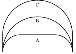
The smoothness aimed for in this thesis is low curvature, undulatory smoothness. Low curvature smoothness means that the curvature of the segments of the path are minimised. Figure 1 (below) shows two paths, path A (left) is of high curvature, whilst path B (right) is of lower curvature, therefore path B is preferable to path A.

Figure 1 Examples of high (A) and low (B) curvature paths.

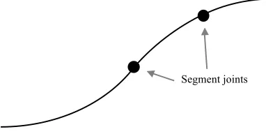
[image:26.595.191.382.601.697.2]

Undulatory smoothness means that no unnecessary loops, kinks, or changes in curvature sign (left or right turns) are present in the path. The diagram below (Figure 2 ) shows an undulatory smooth path, connecting the same two states as are shown the diagram above (Figure 1 ) where the connecting paths are undulatory unsmooth.

Figure 2 Low curvature and undulatory smooth path.

This thesis uses one of two definitions of “unnecessary” dependent on the challenges faced in a particular chapter. If obstacles are not present, then unnecessary means the inclusion of

Segment joints

(27)

loops kinks, or changes in curvature sign are those that may be avoided in forming a path to connect two states. If obstacles are present this is re-defined to mean if these features may be avoided whilst following the edge of an obstacle.

2.7.2 Genericity

Genericity is a property of algorithms that is aimed for to varying degrees for the whole of this thesis, and refers to level of change required to an algorithm’s code in order to handle a particular task or robot. Genericity is useful as an algorithm that requires few changes to its code when changing between tasks and robots is easier to use on a wide range of robots and tasks.

An algorithm with full genericity does not require any changes to be made to the code in order for a particular task to be completed or robot to be controlled. This is infeasible here as it is not possible (by any existing algorithm known to the author) to generate (from scratch) robot specific data, such as kinematics or robot width, or the data provided by each sensor, nor is it possible for an algorithm to control a robot without this information.

An algorithm with no genericity is one that is entirely specific to both a particular robot and task, and any changes to either of these require a complete re-write of all code. It is clearly impractical to use such an algorithm in most real world applications, as it is likely that different tasks may need to be performed, and it may be desirable to use a single algorithm to control many different robots.

As described above, full genericity is impossible to achieve, and zero genericity represents an algorithm that is of little use outside of well-defined production lines. Therefore, the level of genericity achieved by the algorithms described in this thesis will be in between these two extremes and defined within each chapter. The minimum level achieved is applicability to any ground-based robot; the maximum achieved is applicability to any robot for any navigation task in environments that do not contain obstacles. In addition there are no carefully tuned calibration values used in any part of this thesis, as the presence of such values would obviously represent an approach that was not generic.

2.8 Drift & Robustness

Drift is a generic term the occurrence of which is defined here as the robot’s movements differing from those expected by an algorithms’ plan. Drift has many causes, these may be internal to the robot, or external [87]. Internal errors may result from the actuators moving incorrectly, inaccuracies in the model describing the robot, or errors due to poorly calibrated sensors. External error sources include side winds, slippage of the robots wheels on the travel surface, and sensor error due to materials in the environment undesirably reflecting, absorbing or delaying sensor rays.

Drift is present in almost all real-world robotics in some form. The algorithms described in this thesis all attempt to cater for drift in some form, and together cater for all forms of spatial drift.

(28)

Crosswind direction

Desired path Actual path Increasing drift with distance travelled

Initial state

Figure 3 Figure showing the categories of drift, an arrow depicts a sub-category.

[image:28.595.186.398.70.274.2]

Drift has two main varieties: spatial and temporal. Spatial drift in a variable is proportional to the amount a variable is changed; therefore if there is no change in a variable there will be no drift in that variable. Spatial drift may be visualised as the effect of a crosswind on a moving car. If the car has only moved a few meters, then it will only have been blown a small distance from its planned course. However over the course of a mile it will have suffered from a large deviation if no correction is applied (Figure 4 ).

Figure 4 Diagram to illustrate the increase in the spatial drift experienced with distance travelled.

There are two subsets within spatial drift, these are: “power-through” and “wheel-slip”. Power-through drift is drift whereby the correct response is to push harder (i.e. apply more power in order to resist the drift). A crosswind is an example of this kind of drift, as steering into the wind (i.e. applying more power in this direction) is the correct course of action to counteract it. There are however types of spatial drift for which the correct response is not to apply more power. An example of this is wheel spin as this is caused by excessive acceleration; therefore applying more acceleration is not the correct way to counter this drift.

A new, robust, and generic method for the quick creation of smooth paths and near time optimal path tracking

NEAR TIME-OPTIMAL PATH TRACKING

Matthew Bott

A Thesis Submitted for the Degree of PhD

at the

University of St. Andrews

2011

Full metadata for this item is available in

Research@StAndrews:FullText

at:

http://research-repository.st-andrews.ac.uk/

Please use this identifier to cite or link to this item:

http://hdl.handle.net/10023/2095

This item is protected by original copyright

A new, robust, and generic method for

the quick creation of smooth paths and

near time-optimal path tracking

Matthew Bott

School of Computer Science

University of St Andrews

Abstract

Acknowledgements

Declaration

Contents

Chapter 1 – Introduction

1.1

Chapter Overview

1.2

Motivation

1.3

Thesis Objectives

1.4

Contributions

1.5

Thesis Structure

1.6

Publications

Chapter 2 – Background

2.1

Chapter Overview

2.2

A Brief History Of Autonomous Robotics

2.3

Path Tracking and Path Planning

2.3.1

Path Tracking

2.3.2

Path Planning

2.3.3

Suitability Comparison (Planning vs. Tracking)

2.4

Algorithm Design Considerations

2.4.1

Success Criteria

2.4.2

Available Data

2.4.3

Computational Power

2.5

Kinematic and Dynamic Modelling

2.5.1

Forward and Inverse Kinematic Models

2.6

Holonomic and Non-holonomic Constraints

2.7

Smoothness and Genericity

2.7.1

Smoothness

2.7.2

Genericity

2.8

Drift & Robustness