Robust and powerful tests for nonlinear deterministic components
Sam Astilla, David I. Harveyb, Stephen J. Leybourneb and A.M. Robert Taylorc a. Department of Economics, University of Warwick.
b. Granger Centre for Time Series Econometrics and School of Economics, University of Nottingham.
c. Essex Business School, University of Essex.
May 2014
Abstract
We develop a test for the presence of nonlinear deterministic components in a univariate time series, approximated using a Fourier series expansion, designed to be asymptotically robust to the order of integration of the process and to any weak dependence present. Our approach is motivated by the Wald-based testing procedure of Harvey, Leybourne and Xiao (2010) [Journal of Time Series Analysis, vol. 31, p.379-391], but uses a function of an auxiliary unit root statistic to select between the asymptotic I(0) and I(1) critical values, rather than modifying the Wald test statistic as in Harveyet al.. We show that our proposed test has uniformly greater local asymptotic power than the test of Harveyet al. when the shocks are I(1), identical local asymptotic power when the shocks are I(0), and also improved …nite sample properties. We also consider the issue of determining the number of Fourier frequencies used to specify any nonlinear deterministic components, evaluating the performance of algorithmic- and information criterion-based model selection procedures.
Keywords: Trend function testing; Robust tests; Fourier approximation. JEL Classi…cation: C22.
1
Introduction
The ability to detect the presence and magnitude of deterministic components in a …nancial or
eco-nomic time series is of key importance when conducting empirical analysis, particularly for the purposes
of forecasting and testing for a unit root. For example, in the latter case, failure to correctly specify a
relevant deterministic component present in the data is known to result in non-similar and (usually)
inconsistent tests. Moreover, the power of unit root tests to reject the null under the I(0) alternative
when deterministic components are unnecessarily included in a model speci…cation is also reduced.
Traditionally, attention in the literature has focused on a linear deterministic component, most
often the case of a constant and/or linear trend. The possibility of breaks in such linear deterministics
has also received considerable attention, due in particular to the e¤ect these breaks have on standard
unit root and stationarity tests; see,inter alia, Perron (1998). However, as noted by Harvey, Leybourne
and Xiao (2010) [HLX hereafter], these may not necessarily take the form of an instantaneous break
in the trend function. They note that changes in economic aggregates are a¤ected by the response of a
large number of potentially heterogeneous individuals who are unlikely to respond instantaneously to
shocks. As a consequence, they suggest that a smoothly evolving nonlinear deterministic component
might provide a better approximation to the underlying deterministic component of these aggregates.
One possible method to capture such nonlinear behaviour is to approximate the deterministic
component using a Fourier series expansion. This approach is explored by Becker et al. (2004) and
is found to provide a good approximation for a variety of functions. Enders and Lee (2012) show
that modelling the deterministic components of an economic time series via a Fourier function can
approximate changes of various forms, such as a number of sharp breaks or deterministic smooth
transitions, e.g. exponential or logistic smooth transtions (ESTR or LSTR). Becker et al. (2004)
derive a test for the presence of nonlinear deterministic components using a Fourier expansion under
the assumption that the shocks are I(0). Enders and Lee (2012) propose a corresponding test under the
assumption that the data are I(1). The practical implementation of these tests is clearly problematic
since both assume the order of integration of the data to be known. This results in a circular testing
problem as we would need to know the order of integration of our data before performing the tests of
either Becker et al. (2004) and Enders and Lee (2012); however, in order to perform a unit root or
stationarity test we would need to specify the form of the deterministic component.
Motivated by this problem, and drawing on the robust linear trend tests of Vogelsang (1998),
HLX suggest a test that is robust to the order of integration of the data, thereby eliminating this
circular testing problem. This is achieved by using a composite statistic based around a Wald statistic
(that has a well de…ned limit distribution for both I(0) and I(1) shocks) multiplied by a function of
an auxiliary unit root test statistic. This function is speci…ed such that when the shocks are I(0) it
converges in probability to one, leaving the asymptotic distribution of the Wald statistic una¤ected,
but when the shocks are I(1), it converges to a well-de…ned limit distribution. Judicious choice of the
precise function to be used then allows the asymptotic critical values of the composite test statistic to
be lined up in the I(0) and I(1) environments, for a given signi…cance level. This approach therefore
yields tests that display correct asymptotic size for both I(0) and I(1) shocks.
Here we propose an alternative to the methodology of HLX. In our approach a function of an
auxiliary unit root test statistic is used to select between the asymptotic I(0) and I(1) critical values
for the Wald test, rather than creating a composite test via multiplication with the Wald statistic as
in HLX. The motivation underlying this is that the presence of the multiplicative function of a unit
root test statistic in the HLX procedure impacts negatively on the local asymptotic power when the
shocks are I(1), relative to a test that compares the unmodi…ed Wald statistic with its asymptotic I(1)
critical value directly. In contrast, the approach considered in this paper always uses the Wald statistic
without modi…cation, and ensures that the correct asymptotic critical value is used, appropriate to
as the HLX test in the I(0) setting, while delivering (often substantial) local asymptotic power gains
for I(1) shocks. The new approach also provides improved …nite sample behaviour.
The paper is organized as follows. Section 2 outlines the model and the hypotheses of interest,
with the HLX procedure reviewed in section 3. Section 4 presents our new approach, with the limiting
null distribution and local asymptotic power of the tests detailed in section 5. Section 6 addresses
issues related to the practical implementation of the new procedure, and section 7 reports results of
Monte Carlo simulations to assess the …nite sample properties of the proposed tests for a given number
of frequencies in the Fourier expansion. In section 8 we examine the issue of selecting the number of
frequencies to include in the Fourier expansion, and compare the performance of a selection algorithm
based on the proposed tests with one based on the tests of HLX and also an information criterion
approach. Section 9 reports results from an empirical study where the procedures considered in this
paper are applied to a number of …nancial volatility indices, while section 10 concludes.
2
The Model and Testing Hypotheses
Following HLX, we consider a sample of T observations generated according to the following data
generating process (DGP)
yt=dt+ n
X
f=1
1f;Tsin
2 f t
T +
n
X
f=1
2f;Tcos
2 f t
T +ut; t= 1; :::; T: (1)
The nonlinear deterministic component of yt is speci…ed using a Fourier series expansion with the maximum number of frequencies contained in the expansion denoted by n, and f 2 Z+ denoting a
particular frequency. A linear deterministic component is contained in dt, the two leading cases of which aredt= (a constant) anddt= + t (a constant and a linear trend).
We allow the stochastic component,ut, to be either I(0) or I(1), satisfying either Assumption I(0) or Assumption I(1), respectively, below.
Assumption I(0) The stochastic process ut is such that ut = vt, where the process fvtg satis…es
vt = C(L)"t; C(L) := P1i=0CiLi; C(1)2 >0 with P1i=0ijCij< 1, and where "t is a mean zero i.i.d. sequence with E("2
t) = 2" and …nite fourth moment. The long run variance of vt is de…ned as !2v := limT!1T 1E(PtT=1vt)2= 2"C(1)2.
Assumption I(0) ensures that we can apply a Functional Central Limit Theorem (FCLT) to the partial
sums of fvtg; i.e., T 1=2Pbt=1rTcvt !d !vW(r) where b:c denotes the integer part of its argument, !d denotes weak convergence and W(r) is a standard Wiener process.1 When the process is I(0) we
make the following assumption on the Fourier coe¢ cients; 1f;T := 1f!vT 1=2, 2f;T := 2f!vT 1=2, f = 1; :::; n. The T 1=2-scalings on the Fourier coe¢ cients are analytical devices that provide the appropriate Pitman drifts for the local asymptotic power analysis that follows. The scaling by!v is a
1
We maintain the assumption that"t is i.i.d. for consistency with the assumptions in HLX, however, the asymptotic
convenience device that allows the long run variance to be factored out of the limit distributions that
arise for the test statistics outlined in this paper.
Assumption I(1) The stochastic process ut is such that ut = vt, where the process fvtg is as
de…ned in Assumption I(0).
When the process is I(1) we assume that the Fourier coe¢ cients satisfy, 1f;T := 1f!vT1=2, 2f;T := 2f!vT1=2,f = 1; :::; n, with the T1=2-scalings now representing the appropriate Pitman drifts.
In the context of (1), when testing for the presence of nonlinear deterministic components our null
and alternative hypotheses are given by
H0: 1f;T = 2f;T = 0; f = 1; :::; n
H1:at least one of 1f;T; 2f;T 6= 0; f = 1; :::; n:
Under H0 the deterministic component in (1) reduces to dt, while H1 speci…es that some form of
nonlinear deterministic component is present in the data. The formulation of H1 allows for the case
where 1f;T = 2f;T = 0 for some but not all frequencies f = 1; :::; n.
3
The HLX Test
In order to construct tests that are robust to whether the shocks are I(0) or I(1), HLX …rst consider
the partially summed counterpart to regression (1)
zt= t
X
s=1 ds+
n X f=1 1f;T t X s=1
sin 2 f s
T + n X f=1 2f;T t X s=1
cos 2 f s
T + t (2)
wherezt:=Pts=1ysand t:=
Pt
s=1us. They then consider a scaled Wald statistic forH0 againstH1 based on (2), of the formSW0n:= (RSSR RSSU)=RSSU, whereRSSR denotes the residual sum of squares from OLS regression of zt on Pts=1ds, and RSSU denotes the residual sum of squares from OLS estimation of the unrestricted regression (2). The notationSW0nindicates we are testing the null of zero frequencies against the alternative of up to nfrequencies.
The limit distribution of SWn
0 depends on whether Assumption I(0) or Assumption I(1) holds, but crucially it is well de…ned in each case. Consequently, HLX propose a Vogelsang (1998)-type
modi…cation, basing their recommended test on the modi…ed statisticM W0n:=SW0nexp( b jDFj 1), where b is a …nite positive constant and DF is the Dickey-Fuller t-statistic applied to the residuals
^
ut obtained from OLS estimation of (1), i.e. DF = (^ 1)=s:e:(^) with ^ obtained from the OLS regression
^
ut= u^t 1+ p
X
i=0
i u^t i+et: (3)
the limiting null distributions of SW0n under I(0) and I(1) shocks asD0 andD1, respectively, it then follows that, under H0, M W0n
d
! D0 under Assumption I(0) and M W0n d
!D1exp( b jUj 1) under Assumption I(1). The constant b is chosen such that, for a given signi…cance level , theM W0n test has the same asymptotic critical value under I(0) and I(1) shocks. As a result, the M Wn
0 test will have the correct size asymptotically regardless of whether Assumption I(0) or Assumption I(1) holds.
4
An Alternative Robust Test
Our proposed testing procedure involves utilising the same scaled Wald statistic as HLX, namely
SW0n, but we propose using an auxiliary unit root statistic (denoted by J) to switch between the critical values appropriate for SWn
0 under Assumption I(0) and Assumption I(1), i.e. critical values from D0 and D1, respectively, rather than modifying the test statistic itself with the multiplicative
term exp( b jDFj 1) as in HLX. Such an approach has the advantage that it leads to a test with
local asymptotic power identical to the tests of HLX when the shocks are I(0), but with greater local
asymptotic power when the shocks are I(1) due to the removal of the in‡uence of the auxiliary unit
root test statistic on the asymptotic distribution of the test in the I(1) case.
Denoting by cv0; and cv1; the -level critical values from D0 and D1, respectively, we wish to compareSWn
0 withcv0; when the shocks are I(0), and SW0n withcv1; when the shocks are I(1). To achieve this, we consider the following adaptive critical value
cv := J; cv0; + (1 J; )cv1; ; J; := exp( T J) (4)
with and positive constants. We require a value of and a statistic J such that T J converges
in probability to zero under Assumption I(0) but diverges to positive in…nity under Assumption I(1).
Then, when the shocks are I(0), J; p
! 1 and cv !p cv0; , and when the shocks are I(1), J; p ! 0 and cv !p cv1; . This ensures that the correct critical value is used asymptotically, yielding a robust testing approach. Note that although the constant will play a role in the …nite sample behaviour
of J; , it is asymptotically irrelevant. In what follows, we denote by ASW0n our proposed test that compares the statisticSW0nwith the adaptive critical valuecv , given suitable choices of andJ that satisfy our requirements onT J.
5
Asymptotic Results
De…ning := [ 11; :::; 1n; 21; :::; 2n]0,Xk(r) := [m11(r); :::; m1k(r); m21(r); :::; m2k(r)]0, andHk(r) :=
[F(r);sin(2 r); :::;sin(2 kr);cos(2 r); :::;cos(2 kr)]0, where F(r) := 1 if dt = , F(r) := (1; r) if dt= + t, m1f(r) := 21f(1 cos(2 f r)) and m2f(r) := 21f sin(2 f r), the following large sample results obtain (see HLX for the limits of M W0n; the limits for SW0n follow in a straightforward way). Ifyt is generated by (1) under H1, then
(a) Under Assumption I(0), SW0n,M W0n!d
R1
0 LR(r; ) 2dr
R1
0 LU(r)2
whereLR(r; )denotes the continuous time residuals from the projection of 0Xn(r) +W(r) onto the space spanned by R0rF(s)ds, and LU(r) denotes the continuous time residuals from the projection of W(r) onto the space spanned by[R0rF(s); Xn(r)0]; and
(b) Under Assumption I(1), SW0n !d
R1
0 NR(r; ) 2dr
R1
0 NU(r)2
1 =:D1( )
M W0n !d D1( ) exp( b jUj 1)
whereNR(r; )denotes the continuous time residuals from the projection of 0Xn(r)+
Rr
0 W(s)dsonto the space spanned byR0rF(s)ds,NU(r) denotes the continuous time residuals from the projection of
Rr
0 W(s)dsonto the space spanned by[
Rr
0 F(s); Xn(r)0], andU := (K(1)
2 K(0)2 1)=(2qR1
0 K(r)2dr), withK(r)the continuous time residuals from the projection ofW(r)onto the space spanned byHn(r)0. The asymptotic null distributions of SW0n and M W0n obtain by setting = 0 in the foregoing representations, so that, linking with the notation of the previous section, D0 D0(0) and D1
D1(0). Note that D0 and D1 are functions of n, and thus the limit distribution of SW0n depends on the choice of n. The asymptotic critical values of the with-constant SW0n (dt = ) and with-trend SW0n (dt = + t) statistics, for n = 1;2;3 and for both I(0) and I(1) shocks, are given in Table 1. These were obtained from direct simulation of these limiting distributions, with the Wiener
process approximated using N IID(0;1) random variates, and with the integrals approximated by
normalized sums based on 1,000 steps. Here and throughout the paper, all Monte Carlo simulations
were conducted in Gauss 9.0 using 50,000 replications. The critical values reported for the I(0) case
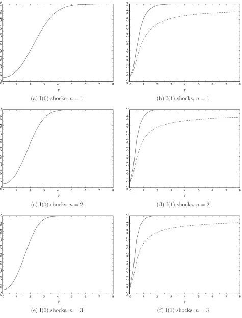
are also the limit critical values ofM W0n, and coincide with the values reported in Table 1 of HLX. Under Assumption I(0), both the M W0n and ASW0n tests share the same asymptotic distribution and, as such, will possess identical local asymptotic power functions. Under Assumption I(1), however,
their local asymptotic power functions di¤er. Henceforth, we will concentrate attention on the
with-constantASWn
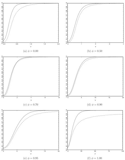
0 test to facilitate direct comparison with the results presented in HLX. Corresponding results for the with-trend variant are available on request. Figure 1 reports the local asymptotic
power (at the nominal 0.05 signi…cance level) under both Assumption I(0) and Assumption I(1) for
n= 1;2;3, with the results again obtained from direct simulation of the limiting distributions. Due
to the multi-parameter nature of the testing problem we present results under the alternative that
11 = ::: = 1n = 21 = ::: = 2n = . Panels (a), (c) and (e) con…rm that the local asymptotic powers of both tests are identical when the shocks are I(0). However, when the shocks are I(1), Panels
(b), (d) and (f) reveal a distinct power ordering between the two test procedures across all values of
n. The new ASW0n test has uniformly superior local asymptotic power to the M W0n test, with the potential power gains being quite substantial. Indeed, we …nd that the maximum power gains across
6
Practical Implementation of the Test Procedure
To implement theASW0ntest, we require choices for andJ which satisfy the conditions onT J given below (4). We followed HLX and experimented with functions of the Dickey-Fuller-type statistic,DF,
and also a Breitung (2002)-type variance ratio unit root statistic
B:=su2T 3 T
X
t=1 t
X
s=1 ^
us
!2
(5)
where s2u := T 1PtT=1u^2t, with ut^ the residuals obtained from OLS estimation of (1). While all choices of and J that satisfy the required conditions onT J result in asymptotically equivalent test
procedures, we found the best overall …nite sample behaviour was achieved when setting = 1=2 and
J =B. With these choices, following results in Breitung (2002), under Assumption I(0) we …ndB =
Op(T 1)and soT1=2J =Op(T 1=2), while under Assumption I(1),B =Op(1)withT1=2J =Op(T1=2), clearly satisfying the required conditions on T J. We recommend these settings for and J in the
implementation of the test.
While the adaptive critical value cv of (4) delivers an appropriate critical value forSW0n asymp-totically, we also consider a …nite sample adjustment that proves to be bene…cial in controlling the new
test’s size in small samples. Results from unreported simulations showed that the procedure outlined
thus far has a tendency to exhibit …nite sample over-size when the shocks are I(1), and …nite sample
under-size when the shocks are I(0). We therefore consider a modi…cation designed to in‡ate (de‡ate)
the …nite sample critical value in the I(1) (I(0)) case. Speci…cally, we consider the following adjusted
adaptive critical value in place of (4)
cv ;adj:= J; (1 J; T 1=2)cv0; + (1 J; )f1 + (1 J; )T 1=2gcv1; (6)
where > 0. Note that this has no e¤ect asymptotically as J; T 1=2 p
! 0 under I(0) and (1 J; )T 1=2
p
!0under I(1).
Although and in (6) and (4) have no impact on the asymptotic behaviour ofASW0n, speci…c values of these parameters are required to implement the test in practice, and the choice of these
values a¤ects the test’s …nite sample properties. We calibrated these choices according to a set of
unreported size and power simulations forn= 1;2;3. As a starting point, for a givenn, we restricted
attention to the set of pairings of ( ; ) which delivered a correct empirical size of exactly (for
each of = 0:10,0:05 and 0:01) for the pure unit root case yt="t N IID(0;1),y1 ="1, and for
the sample size T = 300. Among such pairings, increases in (with corresponding decreases in )
were found to reduce the degree of any over-size displayed in stationary scenarios, but at the cost of
decreased …nite sample power. We …rst chose( ; ) such that the test also had empirical size equal
to when yt="t N IID(0;1)and T = 300. In some cases, however, we found that this choice led
to signi…cant size distortions for moving average"t; in such cases, we selected a( ; )pairing with a larger (and therefore smaller ) to reduce the size distortions. Speci…cally, we chose a pairing such
0:014for nominal 0:10- and 0:01-level tests, respectively) across the ARMA(1,1) and ARIMA(0,1,1)
simulation settings considered in section 7.1 below. We advocate tolerating this modest amount of
potential over-size in order to preserve decent …nite sample power levels. The chosen pairings are given
in Table 2, and we recommend these settings for practical applications of the test.
7
Finite Sample Simulations
7.1 Empirical Size
In this section we consider the …nite sample size behaviour of the M Wn
0 and ASW0n tests, focusing on the case n = 1. We generate data according to the following DGP, which allows for stationary
ARMA(1,1) and integrated ARIMA(0,1,1) shocks: yt= yt 1+"t "t 1,t= 2; :::; T, with u1 ="1 and"t N IID(0;1). Table 3 reports the empirical sizes of nominal 0.05-levelM W01 andASW01 tests
for the sample sizesT =f150;300gand serial correlation parameters =f0;0:5;0:7;0:9;0:95;1g and
=f 0:5;0;0:5g. When calculating theDF unit root test statistic required for theM W1
0 procedure, the lag truncation parameter p in (3) was chosen using the modi…ed Akaike information criterion
(MAIC) of Ng and Perron (2001) withpmax = 12(T =100)1=4 , and using the modi…cation of Perron and Qu (2007), as outlined in HLX.
The …nite sample sizes of the two tests follow broadly similar patterns across the di¤erent serial
correlation parameter settings. Both are close to nominal size for I(1) shocks ( = 1), apart from
some over-size observed for ASW01 when T = 150. At the other extreme, when = 0, we see that in
the absence of moving average components ( = 0), the with-constant ASW1
0 test is approximately correctly sized and the with-trendASW01 test is a little under-sized, while some modest size distortions
are observed when 6= 0. On the other hand, theM W01tests are severely under-sized in all cases when
= 0. For stationary but autocorrelated DGPs(0< <1)all tests can be substantially under-sized
in …nite samples. As was observed by HLX, for some values of the tests are more under-sized for
T = 300than forT = 150; unreported simulations con…rm, however, that this phenomenon eventually
vanishes for much larger sample sizes, in line with our asymptotic results. The results of Table 3 show
that the new ASWn
0 tests are generally conservative, and are therefore unlikely to spuriously signal the presence of nonlinear deterministic components when they are in fact absent. Furthermore, while
under-size is apparent for stationary shocks, the degree of this downward size distortion is less marked
for theASW0n tests than for the M W0n tests.
7.2 Empirical Power
To examine the …nite sample power properties of the tests, we generate data according to the DGP
yt = n
X
f=1
sin 2 f t
T +
n
X
f=1
cos 2 f t
T +ut; t= 1; :::; T (7)
withn= 1,u1 ="1 and"t N IID(0;1). Figure 2 presents power curves for nominal 0.05-level with-constantM W1
0 andASW01tests, forT = 150and =f0;0:5;0:7;0:9;0:95;1g. The power curves were computed using a grid of 50 steps of values for from to0 to max, with max =f2;4;8;20;20;100g,
corresponding to the six values of considered.
Figures 2(f) and 3(f) show that when the shocks are I(1), the power of the newASW01test is clearly
superior to that ofM W01, in line with the asymptotic power results in Figure 1. It is reassuring to see
that the power gains observed in the limit are also manifest in …nite samples, with quite substantial
power advantages available through use of ASW01 in the I(1) setting. When the shocks are I(0), the
two tests are asymptotically equivalent, although it is to be expected that their power properties will
di¤er in …nite samples, particularly given the di¤erential …nite sample size results discussed above.
Indeed, Figures 2(a)-2(e) show that di¤erences between theASW01 and M W01 power curves do occur.
The main observation is thatASW01 generally outperformsM W01 under I(0) shocks. The power gains
associated withASW01 are most marked when = 0, where it is evident that the under-size associated
withM W01 in this case has a detrimental impact on power relative to the better sizedASW01 test. A
similar, albeit less exaggerated, pattern is seen when = 0:5, while there is little to choose between
the two tests when = 0:7 and = 0:9. Finally, when = 0:95, relative power gains are again
displayed byASW01. In summary, theASW01test o¤ers valuable improvements in …nite sample power
relative to M W01, both in the case of I(1) shocks (as would be expected) and also in the case of I(0)
shocks where the tests are asymptotically equivalent.
As suggested by a referee, an alternative to using u^t in the construction ofB would be to instead use residuals obtained from (1) but with the null hypothesis imposed, i.e. to use residuals from OLS
estimation of yt=dt+ut,t= 1; :::; T. It can be shown thatcv ;adj computed usingB based on such restricted residuals has exactly the same asymptotic properties as cv ;adj in (6) under Assumption I(0) and Assumption I(1), both under the null and under the respective local alternative hypotheses.
Unreported simulations show that this approach tends to be susceptible to a greater degree of
under-size than our suggested procedure, while neither procedure dominates the other across in terms of
…nite sample power. As a result, we do not pursue this alternate approach further here.
8
Determining The Number Of Frequencies
The analysis in the previous section assumed that the true maximum number of frequencies, n, was
known. In practice, however, this setting is unknown and must be speci…ed by the practitioner.
Unreported simulation results show that incorrectly specifying the number of frequencies,n, to include
in the testing procedure has a detrimental e¤ect on the power of all of the tests considered in this
paper. For instance, if we choose to perform a test for at mostn+ 1frequencies when the true number
of frequencies is n we will sacri…ce power due to over-speci…cation in the test procedure; similarly,
under-speci…cation ofn can result in tests with very low power.
of frequencies to include in their testing procedure. This algorithm can also be applied to the new
testing approach proposed in this paper. As part of the algorithm, HLX develop a test of the null of
at mostm 1 frequencies versusm frequencies, i.e., within the context of (1),
H0 : 1m;T = 2m;T = 0; 1f;T; 2f;T; f = 1; :::; m 1unrestricted H1 : at least one of 1m;T; 2m;T 6= 0
They recommend the testM Wm
m 1:=SWmm 1exp( b jDFj
1), whereSWm
m 1 := (RSSR RSSU)=RSSU withRSSR and RSSU the restricted and unrestricted residual sums of squares from OLS estimation of (2) with n replaced by m 1 and m, respectively, and where DF is the Dickey-Fuller t-statistic
applied to the OLS residuals from estimation of (1) withn replaced bym.
The new approach proposed in this paper can also be used to construct a test of H0 against
H1. Speci…cally, we adopt the same SWmm 1 statistic that appears as a component in M Wmm 1, and compare this statistic with the adjusted adaptive critical value cv ;adj taking the form of (6), where J; is as de…ned in (4) with = 1=2 and J = B where B now denotes the statistic in (5) with u^t being the residuals from OLS estimation of (1) withn replaced bym.
The following large sample results for SWmm 1 can be obtained directly from HLX. When yt is generated by (1) underH1,
(a) Under Assumption I(0), SWmm 1 !d
R1
0 LR(r; )2dr
R1
0 LU(r)2
1 =:D0( )
where := [ 1m; 2m], LR(r; ) denotes the continuous time residuals from the projection of 1mm1m(r)+ 2mm2m(r)+W(r)onto the space spanned by R0rF(s)ds; Xm 1(r)0 , andLU(r)denotes the continuous time residuals from the projection ofW(r)onto the space spanned by R0rF(s)ds; Xm(r)0 ; and
(b) Under Assumption I(1), SWmm 1 !d
R1
0 NR(r; )2dr
R1
0 NU(r)2
1 =:D1( )
whereNR(r; )denotes the continuous time residuals from the projection of 1mm1m(r)+ 2mm2m(r)+
Rr
0 W(s)dsonto the space spanned by
Rr
0 F(s)ds; Xm 1(r)0 , and NU(r)denotes the continuous time residuals from the projection of R0rW(s)ds onto the space spanned by R0rF(s)ds; Xm(r)0 .
The asymptotic distributions under the null H0 follow by setting = 0 in the above limits.
Asymptotic critical values forSWmm 1 form= 2;3under both Assumption I(0) and Assumption I(1) are given in Table 1. We also determined suitable values for and to be used in constructing
cv ;adj, and these recommended values are given in Table 2. Hereafter we denote byASWmm 1the new tests that compareSWmm 1 with cv ;adj.
Following the HLX algorithm, the ASWn
0 and ASWmm 1 tests can now be used to determine the number of frequencies, n. Given an assumption on the largest possible value of n, nmax, we …rst
conduct the testsASW0i,i= 1; :::; nmax, and if none of these tests reject we concluden= 0. If any of the tests do reject, we identify the largest value of i for which the null is rejected and setm to this
value that nmight take. We then consider ASW0m 1, and if this test fails to reject we set n=m. If, however,ASW0m 1does reject we then perform theASWm
m 1test; then if this test rejects we conclude n=m, otherwise we reducem by one and repeat the loop. For a diagrammatic representation of the
algorithm, see Figure 3 of HLX.
A natural alternative approach to identifying the number of frequencies present in a series would
be a standard model selection criterion. As such we also consider a Bayesian information criterion
(BIC) approach, which for the constant case (dt= ) is based on the following two regressions
yt = + yt 1+ n
X
f=1
1f;Tsin
2 f t
T +
n
X
f=1
2f;Tcos
2 f t
T +
k
X
i=0
ci yt i+et (9)
yt = n
X
f=1
1f;Tsin
2 f t
T +
n
X
f=1
2f;Tcos
2 f t
T +
k
X
i=0
ci yt i+et: (10)
Consider selecting n by minimising the BIC across n =f0;1; :::; nmaxg and k= f0;1; :::; kmaxg for a
given regression. BIC based on (9) will be appropriate when the shocks are I(0), while BIC based on
(10) will be appropriate for I(1) shocks. Consequently, we propose minimising the BIC jointly over
both regressions (9) and (10), and it this procedure with which we will compare the performance of
the HLX-type algorithm below.
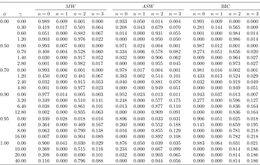
We now assess, by means of Monte Carlo simulation, the relative performance of the HLX algorithm
based on M W0n and M Wmm 1 (which we refer to as M W), the same algorithmic approach based on ASW0n andASWmm 1 (which we denote byASW), and the BIC procedure outlined above. Note that all tests were performed for the with-constant variants and were conducted at the nominal 0.05-level.
Data were generated according to (7)-(8) with n = 2. We compute the frequency with which each
procedure correctly selectsn= 2, along with the frequencies with which each of the incorrect selections
of n= 0;1;3 are made. The choicesnmax= 3 and kmax= 4 are adopted in all cases, and we consider
experiments withT = 150, =f0;0:5;0:7;0:9;0:95;1g, as before. For each value we report results for
four di¤erent values of , including the case = 0. Results for serially correlated"t were found to be
similar to those for i.i.d. innovations and are available upon request.
The results are reported in Table 4. Comparing …rst the two algorithmic approaches, we observe
thatASW generally outperformsM W, in line with the superior …nite sample testing properties that
the constituent tests involved in ASW display. Due to the inherent multiple testing issues with the
algorithms, when = 0 we see that bothASW and M W select a non-zero value of nwith frequency
greater than the nominal level, less so in the case ofM W due to its lower …nite sample size. However, as
might be expected from the results of section 7, when >0theASW approach generally outperforms
theM W approach in terms of the frequency with which n= 2 is selected. Indeed, the improvements
o¤ered by ASW over the original M W are quite substantial in a number of cases, particularly for
modest values of . While M W can outperform ASW, such gains are always relatively minor, and
tend to occur in situations where both procedures selectn= 2with high probability.
Turning our attention to a comparison ofASW with the BIC approach, it can be seen that when
ASW. In some cases, di¤erences are seen, but neither procedure dominates the other overall when
there are truly no nonlinear deterministic components present. When >0, we …nd that neitherASW
nor BIC dominates the other across the di¤erent magnitudes considered. While the performance of
the two methods for determining the number of frequencies can be quite di¤erent for any given DGP,
these di¤erences do not follow a systematic pattern across all or ; as such, it is di¢ cult to argue
for a particular ranking betweenASW and BIC. What is clear, however, is that both procedures o¤er
improvements relative to theM W approach of HLX.
The previous simulation study has examined the ability of the proposed algorithms and BIC
procedure to correctly specifynwhen the deterministic component of the series is exactly approximated
by a Fourier series expansion. It is also important to investigate how useful these approaches are in
approximating other forms of nonlinear deterministic components. To that end we generated data
according to yt = dt+ut, t = 1; :::; T, with ut as in (8) for = f0;0:5;1g, and with dt speci…ed
as either a mid-sample ESTR, i.e. dt = [1 exp( 0:1(t 0:5T)2)], or as a mid-sample LSTR, i.e. dt= =[1 +exp(0:1(t 0:5T))]. For a sample size of T = 150 we compute the power of the methods
to detect nonlinear deterministic elements, measured as the percentage of replications for which the
ASW algorithm or BIC selects n >0 frequencies. Table 5 reports, for a range of magnitudes, the
power of with-constantASW and BIC (results are omitted forM W as its performance was uniformly
worse than ASW). For ESTR deterministics, both ASW and BIC have power that is increasing in ,
indicating that the Fourier approximation works reasonably well in terms of modelling the ESTR-type
nonlinearities. Of the two procedures, BIC o¤ers higher power than ASW, particularly when >0.
In the case of LSTR deterministics, however, the powers of both with-constant ASW and BIC
are typically decreasing in (with the exception of BIC when = 1), so while we again …nd that
BIC outperformsASW here, neither procedure performs well across all values of considered. This
feature arises since the LSTR component involves a relatively slow transition from one level to another,
which is not well modelled by the Fourier terms of frequencyf = 1;2;3 that are included in the …tted
unrestricted model (this approximation error may also be magni…ed in the ASW procedure due to
the statistics being based on the partially summed regression (2)). To capture these low frequency
movements, one would need to incorporate Fourier terms with lower frequency than one, e.g. f = 0:5,
in the approximation. Of course, such low frequency Fourier terms can themselves be reasonably well
approximated by a linear trend term, hence we also report in Table 5 results obtained from application
of the with-trend version of ASW to the LSTR data generating processes. We see that for the cases
where the with-constantASW su¤ered from very low power, the with-trend variant has decent power
which is also now increasing in the magnitude of . We also see in Table 5 that with-trendASW also
delivers some power improvements over with-constant ASW in the ESTR simulations, particularly
when = 1. It appears, therefore, that when low frequency changes are present in the data, the
with-trend variant ofASW is a potentially more robust approach for detecting deterministic nonlinearities,
9
Empirical Application
There has been much interest in the …nancial literature in modelling the volatility of economic
in-dicators, most notably …nancial indicators such as stock market indices. While early work by, inter
alia, Poterba and Summers (1986), Frenchet al. (1987) and Schwert and Seguin (1990) concentrated
on modelling volatility in stock market indices using linear methods, more recent work by Cao and
Tsay (1992) attempts to use nonlinear methods to analyse such indices using threshold autoregressive
and nonlinear GARCH and EGARCH models. Such methods assume that any observed nonlinearity
in the volatility indices is stochastic rather than deterministic. It is of interest, however, to assess
whether we can detect nonlinear behaviour in thedeterministic components of such volatility indices.
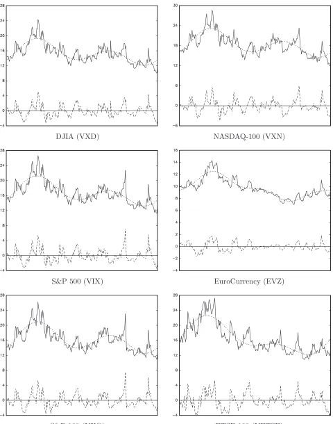
To that end we collected daily data on six volatility indices for the one year period ending 18
March 2013. Five of these indices measure the volatility of a particular stock market index: the Dow
Jones Industrial Average Volatility Index (Ticker: VXD), the NASDAQ-100 Volatility Index (VXN),
the S&P 500 Volatility Index (VIX), the S&P 100 Volatility Index (VXO) and the FTSE 100 Volatility
Index (VFTSE). The …nal series considered is the EuroCurrency Volatility Index (EVZ), which is an
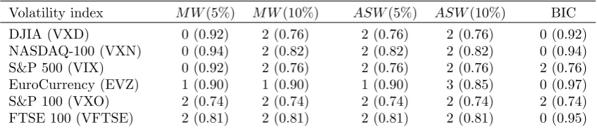
index of the volatility of the US$/EUR exchange rate. We applied the with-constant ASW andM W
algorithms described in section 8 (withnmax= 3), implemented at both the 0.05 and 0.10 signi…cance
levels, to each series. We also applied the BIC selection procedure as a point of comparison. The
number of frequencies, ^n, detected by these methods are reported in Table 6. In all cases, some form
of nonlinear deterministic behaviour is detected in the volatility indices, suggesting a consistent body
of evidence for nonlinear behaviour in the deterministic components of these …nancial volatility series.
The pattern of results observed in Table 6 is consistent with the …nite sample simulations presented
in sections 7 and 8. In all cases, for a given signi…cance level, ASW choosesn^ to be greater than or
equal to that chosen byM W; indeed there are three series for whichM W does not …nd any evidence
of nonlinearity at the 0.05-level, whileASW selectsn^= 2. In comparison with the BIC procedure, we
…nd that ASW …nds more evidence for deterministic nonlinearity, with BIC selecting ^n= 0 for four
of the series, and never identifying a greater number of frequencies thanASW.
As a measure of the underlying persistence in each series, Table 6 also reports (in parentheses)
the estimate of obtained from the DF regression (3) used in the M W0n statistic, where n is set to the corresponding number of frequencies listed in Table 6. These suggest that the series are highly
persistent around a nonlinear deterministic component, but it is unclear whether the stochastic
com-ponents would be best modelled by stationary or unit root processes. This highlights the advantages
of the robust procedures considered in this paper, as we do not need to take a stand on the integration
properties of the data. Interestingly, …tting only a constant to the data results in estimates of very
close to unity, suggesting that failure to specify the nonlinear deterministic components of these series
could well lead to the inference that they contain a unit root. Note also that since the with-constant
ASW procedure always selectsn >^ 0, it does not appear that problematic low frequency movements
are a feature of these time series.
ASW are presented alongside the original and detrended series in Figure 3. Note that for the EVZ
series we plot the …tted and detrended series forn^= 3rather thann^ = 1. We see that the deterministic
components detected byASW appear to …t the data rather well, with the apparent nonlinear behaviour
in the series well approximated by the Fourier frequency representation in most cases.
10
Conclusions
We have proposed a new approach to testing for the presence of nonlinear deterministic components
in an economic time series designed to be robust to the order of integration of the data and to any
weak dependence present. The recommended approach involves using a scaled Wald statistic that
has well de…ned, but di¤erent, limit distributions depending on whether the stochastic component of
the series is I(0) or I(1). Robustness is achieved by using an adaptive critical value constructed so
that the appropriate I(0) or I(1) critical value is selected asymptotically. This delivers a test with
the same asymptotic properties as the test of HLX in an I(0) environment, but with worthwhile local
asymptotic power gains in an I(1) setting. Monte Carlo simulations suggest that the new test also has
superior overall …nite sample size and power properties to the HLX test for both I(0) and I(1) shocks.
The proposed testing procedure can be employed in the algorithm of HLX to determine the number
of frequencies used to model a series that contains potential nonlinear deterministic components. We
have also considered a model selection approach based on the BIC which was also shown to outperform
the original HLX procedure. Our empirical application to …nancial market volatility indices over the
last year supports the notion that the new procedures o¤er bene…ts over extant methods.
References
Becker, R., Enders, W. and Hurn, S. (2004). A general test for time dependence in parameters.
Journal of Applied Econometrics 19, 899-906.
Becker, R., Enders, W. and Lee, J. (2006). A stationarity test in the presence of an unknown number
of smooth breaks. Journal of Time Series Analysis 27, 381-409.
Breitung, J. (2002). Nonparametric tests for unit roots and cointegration. Journal of Econometrics
108, 343-363.
Cao, C.Q. and Tsay, R.S. (1992). Nonlinear time-series analysis of stock volatilities. Journal of
Applied Econometrics 7, 165-185.
Enders, W. and Lee, J. (2012). A unit root test using a Fourier series to approximate smooth breaks.
Oxford Bulletin of Economics and Statistics 74, 574-599.
French, K.R., Schwert, G.W. and Stambaugh, R. (1987). Expected stock returns and volatility.
Harvey, D.I., Leybourne, S.J. and Xiao, L. (2010). Testing for nonlinear deterministic components
when the order of integration is unknown. Journal of Time Series Analysis 31, 379-391.
Ng, S. and Perron, P. (2001). Lag length selection and the construction of unit root tests with good
size and power. Econometrica 69, 1519-1554.
Perron, P. (1998). Trends and random walks in macroeconomic time series: further evidence from a
new approach. Journal of Economic Dynamics and Control 12, 297-332.
Perron, P. and Qu, Z. (2007). A simple modi…cation to improve the …nite sample properties of Ng
and Perron’s unit root tests. Economics Letters 94, 12-19.
Poterba, J.M. and Summers, L.H. (1986). The persistence of volatility and stock market ‡uctuaions.
American Economic Review 76, 1143-1151.
Schwert, G.W. and Seguin, P.J. (1990). Heteroscedasticity in stock returns. Journal of Finance 45,
1129-1155.
Vogelsang, T.J. (1998). Trend function hypothesis testing in the presence of serial correlation.
Table 1. Asymptoticξ-level critical values forSW0nand SWm−1m statistics
n= 1 n= 2 n= 3
ξ 0.10 0.05 0.01 0.10 0.05 0.01 0.10 0.05 0.01
With-constantSWn 0
cv0,ξ 5.268 7.439 13.370 9.337 12.754 21.495 13.259 17.702 29.159
cv1,ξ 50.631 76.222 167.163 193.162 274.977 565.278 475.264 680.520 1300.226
With-trendSWn 0
cv0,ξ 2.677 3.708 6.370 4.685 6.124 9.921 6.550 8.468 13.308
cv1,ξ 30.601 47.342 103.816 100.248 150.228 295.168 227.125 329.713 644.469
m= 2 m= 3
ξ 0.10 0.05 0.01 0.10 0.05 0.01
With-constantSWm m−1
cv0,ξ 1.779 2.406 4.007 1.038 1.393 2.252
cv1,ξ 9.829 14.138 27.101 4.636 6.437 12.147
With-trendSWm m−1
cv0,ξ 1.310 1.774 2.904 0.856 1.138 1.849
cv1,ξ 8.556 12.624 24.795 4.591 6.513 12.293
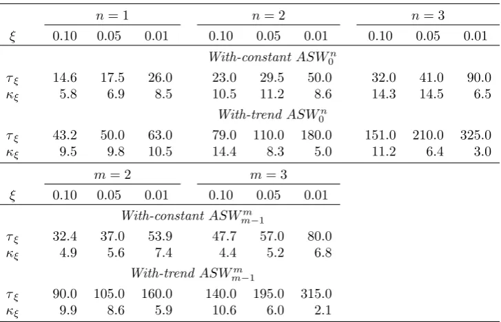
Table 2. τξ and κξ values for ASW0n and ASWm−1m tests
n= 1 n= 2 n= 3
ξ 0.10 0.05 0.01 0.10 0.05 0.01 0.10 0.05 0.01
With-constantASWn 0
τξ 14.6 17.5 26.0 23.0 29.5 50.0 32.0 41.0 90.0
κξ 5.8 6.9 8.5 10.5 11.2 8.6 14.3 14.5 6.5
With-trendASW0n
τξ 43.2 50.0 63.0 79.0 110.0 180.0 151.0 210.0 325.0
κξ 9.5 9.8 10.5 14.4 8.3 5.0 11.2 6.4 3.0
m= 2 m= 3
ξ 0.10 0.05 0.01 0.10 0.05 0.01
With-constantASWm m−1
τξ 32.4 37.0 53.9 47.7 57.0 80.0
κξ 4.9 5.6 7.4 4.4 5.2 6.8
With-trendASWmm−1
τξ 90.0 105.0 160.0 140.0 195.0 315.0
[image:16.595.117.481.391.625.2]Table 3. Finite sample size ofM W01 and ASW01 tests
With-constant tests With-trend tests
T = 150 T = 300 T = 150 T = 300
φ θ M W01 ASW01 M W01 ASW01 M W01 ASW01 M W01 ASW01
0.00 −0.5 0.006 0.033 0.010 0.034 0.002 0.010 0.004 0.014 0.0 0.009 0.051 0.012 0.050 0.004 0.026 0.007 0.032 0.5 0.004 0.057 0.011 0.063 0.001 0.053 0.006 0.068 0.50 −0.5 0.003 0.018 0.004 0.018 0.000 0.003 0.001 0.004 0.0 0.007 0.025 0.008 0.024 0.002 0.007 0.003 0.007 0.5 0.009 0.051 0.012 0.050 0.004 0.026 0.007 0.032 0.70 −0.5 0.002 0.014 0.003 0.011 0.000 0.002 0.001 0.002 0.0 0.006 0.018 0.006 0.014 0.002 0.004 0.002 0.003 0.5 0.008 0.040 0.006 0.033 0.004 0.015 0.003 0.013 0.90 −0.5 0.010 0.022 0.005 0.009 0.002 0.005 0.001 0.001 0.0 0.015 0.025 0.007 0.010 0.005 0.006 0.002 0.002 0.5 0.015 0.045 0.007 0.018 0.006 0.017 0.002 0.005 0.95 −0.5 0.024 0.041 0.011 0.015 0.008 0.014 0.003 0.003 0.0 0.030 0.044 0.013 0.016 0.013 0.016 0.005 0.004 0.5 0.031 0.069 0.014 0.025 0.015 0.032 0.005 0.008 1.00 −0.5 0.039 0.058 0.040 0.049 0.038 0.057 0.039 0.049 0.0 0.047 0.060 0.047 0.050 0.047 0.061 0.047 0.050 0.5 0.049 0.076 0.048 0.058 0.052 0.091 0.049 0.063
Table 4. Number of frequencies selected by with-constant M W and ASW algorithms and BIC:T = 150
M W ASW BIC
φ γ n= 0 n= 1 n= 2 n= 3 n= 0 n= 1 n= 2 n= 3 n= 0 n= 1 n= 2 n= 3
[image:17.595.36.562.428.762.2]Table 5. Power ofASW algorithm and BIC to detect exponential and logistic smooth transitions: T = 150
ESTR LSTR
φ γ ASWc BIC ASWt γ ASWc BIC ASWt
0.0 1.0 0.508 0.526 0.520 2.0 0.484 0.969 0.263 1.5 0.806 0.929 0.837 4.0 0.055 0.428 0.687 2.0 0.936 0.997 0.958 6.0 0.001 0.034 0.895 0.5 3.0 0.588 0.893 0.660 10.0 0.001 0.042 0.474 4.0 0.797 0.990 0.803 15.0 0.000 0.005 0.765 5.0 0.906 0.997 0.922 20.0 0.000 0.026 0.921 1.0 25.0 0.405 0.730 0.868 25.0 0.163 0.332 0.312 50.0 0.701 0.999 1.000 50.0 0.057 0.922 0.698 75.0 0.872 1.000 1.000 75.0 0.011 0.993 0.474
Note: ASWc andASWt denote with-constant and with-trendASW, respectively.
Table 6. Number of frequencies selected by with-constant M W and ASW algorithms and BIC for volatility indices
Volatility index M W(5%) M W(10%) ASW(5%) ASW(10%) BIC
DJIA (VXD) 0 (0.92) 2 (0.76) 2 (0.76) 2 (0.76) 0 (0.92) NASDAQ-100 (VXN) 0 (0.94) 2 (0.82) 2 (0.82) 2 (0.82) 0 (0.94) S&P 500 (VIX) 0 (0.92) 2 (0.76) 2 (0.76) 2 (0.76) 2 (0.76) EuroCurrency (EVZ) 1 (0.90) 1 (0.90) 1 (0.90) 3 (0.85) 0 (0.97) S&P 100 (VXO) 2 (0.74) 2 (0.74) 2 (0.74) 2 (0.74) 2 (0.74) FTSE 100 (VFTSE) 2 (0.81) 2 (0.81) 2 (0.81) 2 (0.81) 0 (0.95)
[image:18.595.86.510.335.427.2](a) I(0) shocks, n= 1 (b) I(1) shocks,n= 1
(c) I(0) shocks, n= 2 (d) I(1) shocks,n= 2
[image:19.595.61.536.95.720.2](e) I(0) shocks, n= 3 (f) I(1) shocks, n= 3
Figure 1. Local asymptotic power of with-constant tests: M Wn
(a)φ= 0.00 (b)φ= 0.50
(c) φ= 0.70 (d)φ= 0.90
[image:20.595.54.538.90.712.2](e) φ= 0.95 (f)φ= 1.00
Figure 2. Finite sample power of with-constant tests: T = 150, n= 1;M Wn
DJIA (VXD) NASDAQ-100 (VXN)
S&P 500 (VIX) EuroCurrency (EVZ)
[image:21.595.61.541.85.695.2]S&P 100 (VXO) FTSE 100 (VFTSE)