Published Online November 2008 in SciRes (http://www.SciRP.org/journal/ijcns/).
Improving Throughput in Wireless Local Area Networks
Imam AL-WAZEDI, Anjali AGARWAL, Ahmed K. ELHAKEEM
Department of Electrical and Computer Engineering,Concordia University, Montreal, Quebec, Canada
Email: [email protected], {aagarwal,ahmed}@ece.concordia.ca Received September 6, 2008; revised October 16, 2008; accepted October 21, 2008
Abstract
The medium access control (MAC) technique of standard WLANs, called the distributed coordination function
(DCF), is carrier sense multiple access based on collision avoidance (CSMA/CA) scheme with binary slotted
exponential backoff. It has a two way handshaking technique for packet transmission and also defines an
additional four way handshaking technique called RTS/CTS mechanism, which is used to reduce the hidden
terminal problem. The RTS/CTS frames carry the information of the packet length to be transmitted which can
be read by any listening stations, to update a network allocation vector (NAV) about the information of the
period of time in which the channel is busy. In this paper a method is proposed called the table driven technique
(which has two parts called table driven DCF and table driven RTS/CTS) which is similar to the standard DCF
(IEEE802.11) and RTS/CTS (IEEE802.11) system without having the exponential backoff. In this technique
users use the optimum transmission probability by estimating the number of stations from the traffic conditions
in a sliding window fashion one period at a time, thereby increasing the throughput compared to the standard
DCF (IEEE802.11) and RTS/CTS (IEEE802.11) mechanism while maintaining the same fairness and the
delay performance.
Keywords: Standard DCF (IEEE802.11), Standard RTS/CTS (IEEE802.11), Table Driven DCF, Table
Driven RTS/CTS
1. Introduction
Wireless local area networks (WLANs) have been widely deployed for the past decade. Their performance has been the subject of intensive research. In [1] an improvement of throughput and fairness is shown by optimizing the backoff without estimating the number of active nodes in the network. In [2], the authors proposed a MAC layer based WLAN technique in which they gave higher priority to access points so as to improve the throughput and the channel utilization. A technique is proposed where the backoff is tuned based on collision avoidance and fairness to improve the channel utilization [3]. In [5] a DCF model is proposed where the arrival and the service of the packets in the queue are controlled to improve the throughput and delay performance.
Cali in [6] pointed out that depending on the network configuration, DCF may deliver a much lower throughput compared to the theoretical limit. Cali derived a distributed algorithm that enables the stations to tune its backoff at run time where a considerable improvement in
the throughput is shown. In [7] a contention based MAC protocol named fast collision resolution is presented where the backoff is also utilized. A model named DCF+ in [8] is proposed which uses the backoff to improve the fairness.
It is evident that the throughput, delay, fairness performances are improved by tuning the backoff in different scenarios considered by the authors in [1–8].
RTS/CTS mechanism with (NAV) is used solve the hidden terminal problem. In [9] Khurana proposed a concept of Hearing graph to model the hidden terminals in static environment and analyzed the performance. Also in [11] Fullmer, proposed a three way handshaking technique to solve the hidden terminal problems of single channel WLANs. However our paper does not concentrate on the hidden terminals but contributes on a modification of the standard DCF and standard RTS/CTS mechanisms.
the use of the exponential backoff. In table driven DCF and table driven RTS/CTS the users estimate the number of active stations and transmit with an optimum probability measured from the traffic conditions (by sensing the channel) in a sliding window fashion, which is described elaborately later on. Simulation results show that our systems out perform the standard in terms of throughput while maintaining same delay and fairness.
2. The IEEE 802.11 MAC Protocol
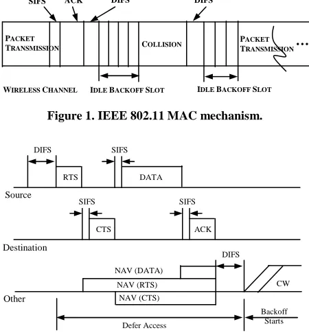
Figure 1 shows one of many transmission scenarios possible with the IEEE 802.11 DCF mode. In this mode a node with a packet to transmit initializes a backoff timer with a random value selected uniformly from the range [0, CW-1], where CW is the contention window in terms of time slots. After a node senses that the channel is idle for an interval called DIFS (DCF interframe space), it begins to decrease the backoff timer by one for each idle time slot observed on the channel. When the channel becomes busy due to other nodes transmission ativity the node freezes its backoff timer until the channel is sensed idle for another DIFS. When the backoff timer reaches zero, the node begins to transmit. If the transmission is successful, the receiver sends back an acknowledgement (ACK) an interval called the SIFS. Then, the transmitter resets its CW to CWmin. In case of collisions the transmitter fails to
receive the ACK from its intended receiver within the specified period, it doubles its CW subject to maximum value CWmax, chooses a new backoff timer, and starts the
above processes again.
[image:2.595.59.284.480.724.2]In 802.11, DCF also provides a more efficient way of transmitting data frames that involves transmission of special
Figure 1. IEEE 802.11 MAC mechanism.
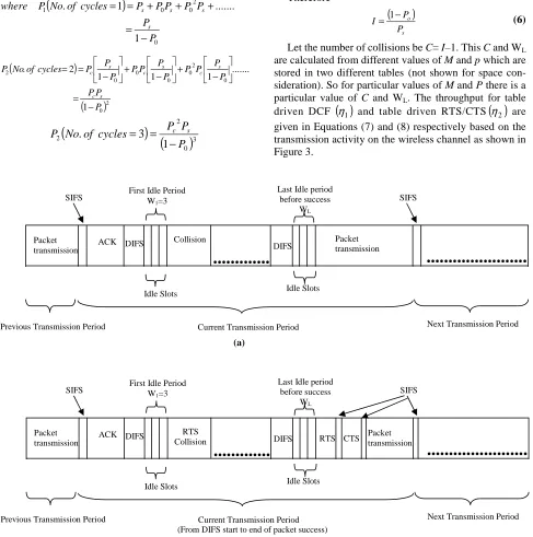
Figure 2. Standard RTS/CTS access mechanism in IEEE 802.11.
short RTS and CTS frames prior to the transmission of actual data frame. As shown in Figure 2, an RTS frame is transmitted by a node, which needs to transmit a packet. When the destination receives the RTS frame, it will transmit a CTS frame after SIFS interval immediately following the reception of the RTS frame. The source station is allowed to transmit its packet only if it receives the CTS correctly. Note that all the other stations are capable of updating their knowledge about other nodes transmission duration by receiving a certain field in RTS, CTS, ACK, and packets transmission called network allocation vector (NAV). This helps to combat the hidden terminal problem. In fact, a node that is able to receive the CTS frames correctly, can avoid collisions even when it is unable to sense the data transmissions directly from the source station. If a collision occurs with two or more RTS frames, much less bandwidth is wasted when compared with the situations where larger data frames in collision, thus justifying the case for RTS, CTS mode of operation [4].
3. Analysis of Table Driven DCF and Table
Driven RTS/CTS
Let p be the transmission probability of each node and M be the number of active stations. Assuming each user tries to transmit randomly in each slot following the DIFS period. According to table driven DCF (Figure 3) the probability of successful transmission, is thus given by Equation (1).
1
) 1
( − −
= M
s Mp p
P (1)
The probability of an idle slot in table driven DCF is
M
o p
P =(1− ) (2)
and the probability of unsuccessful transmission for table driven DCF is
o s
c P P
P =1− − (3)
Let
i
be the number of idle periods (cycles) before a successful transmission as shown in Figure 3 and j be the number of idle slots in each idle period lengths (W1,W2,…). The throughput (η1) is given by Equation (7)for table driven DCF.
It is easily seen that the average length of each idle period except the last one before packet success in table driven DCF is given by
( )
∑
∞ =− = =
= =
1 1
2
1 ... ( )
j
c j o
L E j j P P
W W
W
(
)
21 o
c o
P P P −
= slots (4)
which means Equation (4) determines the number of idle slots before a collision.
The last idle period before a success, has an average of
(
)
21 o
s o L
P P P W
−
= slots (5) RTS
DIFS
DATA SIFS
Source
Destination
Other
SIFS
CTS
SIFS
ACK
DIFS NAV (DATA)
NAV (RTS) NAV (CTS)
Defer Access
CW
Backoff Starts PACKET
TRANSMISSION
SIFS ACK DIFS
WIRELESS CHANNEL IDLE BACKOFF SLOT IDLE BACKOFF SLOT COLLISION
DIFS
PACKET TRANSMISSION…
The average number of cycles (I) is given by,
∑
∞ ==
1 i iiP
I
(
)
0 2 0 0 1 1 ... 1 . P P P P P P P cycles of No P where s s s s − = + + + = =(
)
(
)
2 0 0 2 0 0 0 0 2 1 ... 1 1 1 2 . P P P P P P P P P P P P P P cycles of No P s c s c s c s c − = − + − + − = =(
) ( )
30 2 2
1
3
.
P
P
P
cycles
of
No
P
c s−
=
=
(
)
is i c i
P
P
P
P
0 11
−
=
− Therefore(
)
s o P PI= 1− (6)
Let the number of collisions be C= I–1. This C and WL
are calculated from different values of M and p which are stored in two different tables (not shown for space con- sideration). So for particular values of M and P there is a particular value of C and WL. The throughput for table
driven DCF
( )
η1 and table driven RTS/CTS( )
η2 aregiven in Equations (7) and (8) respectively based on the transmission activity on the wireless channel as shown in Figure 3.
(a)
(b)
Figure 3. Transmission Activity on the Wireless Channel for (a) table driven DCF and (b) table driven RTS/CTS.
(
L)
Slot{
DIFS}
DIFS ACK SIFS Payload L SlotPayload T W T T T T T I T W W W T + + + + + − + + + =
− ( 1)
.. 1
2 1 1
η
(7)
(
L)
Slot{
RTS DIFS SIFS}
DIFS RTS CTS ACK SIFS Payload L SlotPayload T W T T T T T T T T T I T W W W T + + + + + + + + + − + + + =
− ( 1) 3
.. 1
2 1 2
η
(8)
(From DIFS start to end of packet success) Packet
transmission SIFS
ACK DIFS
Idle Slots RTS Collision
...
...
DIFS Idle Slots Packet transmission...
...
Current Transmission Period
SIFS
Previous Transmission Period Next Transmission Period
First Idle Period W1=3
RTS CTS Last Idle period
before success WL
Packet transmission
SIFS
ACK DIFS
Idle Slots Collision
...
...
DIFS Idle Slots Packet transmission...
...
Current Transmission Period
SIFS
Previous Transmission Period Next Transmission Period
First Idle Period W1=3
Last Idle period before success
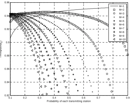
The throughput η1 (for table driven DCF) is calculated for different values of M and p as in Figure 4. Table 1 depicts the probabilities at which the maximum throughput occurs for different values of M.
Similarly for the table driven RTS/CTS, to calculate the C and WL, Equations (1)–(6) are used. However the
throughput is calculated from Equation (8) which includes the RTS/CTS frames (Figure 3).
For the case of table driven RTS/CTS all cycles leading to no success (RTS heard but no CTS) will each have a cost of TRTS+TDIFS+TSlot seconds.
4. Operation of Table Driven Technique
In the proposed protocol, if the nodes sense that the channel is idle for an interval called DIFS (DCF interframe space), they try to send a packet with a proba- bility p, which is dependent on the traffic condition i.e. the number and activities of the nodes, as follows.
A user continuously monitors the channel in each idle slot following the DIFS idle period. If the previous slot is idle, it calls a uniform random generator (0,1). If the value
0.1 0.2 0.3 0.4 0.5 0.6 0.7 0.8 0.9
0.82 0.84 0.86 0.88 0.9 0.92 0.94 0.96
Probability of each transmitting station
T
h
ro
u
g
h
p
u
t(η
1
)
M=1 M=2 M=3 M=4 M=5 M=6 M=7 M=8 M=9 M=10
[image:4.595.60.287.354.533.2]Figure 4. Throughput for different probabilities and different number of stations for table driven DCF.
Table 1. Optimum throughput for different probabilities and different number of stations for table driven DCF.
No of
Stations Probability Optimum throughput
1 0.9000 0.9532
2 0.3400 0.9458
3 0.2200 0.9444
4 0.1600 0.9437
5 0.1300 0.9434
6 0.1000 0.9431
7 0.1000 0.9428
8 0.1000 0.9420
9 0.1000 0.9410
10 0.1000 0.9397
of this generator is less than or equal to p, it tries to start its packet transmission in the given next slot. If the value is larger than p, the user persist on listening and repeats trials as stated. However if the channel is sensed busy the user defers his transmission till the next DIFS idle period heard.
The users measure the number of collisions C= I–1 and the length WL by monitoring the channel over a large
enough window (which is explained latter on). With the help of these values the users can use the tables formulated in Section 3 to obtain the corresponding p and M.
Users having a non-empty queue start by monitoring the channel for the first n transmission periods. This active user will average the length of the idle period preceding the correct packet transmission over n transmission periods, i.e. WL and C, the average number of collisions over the same period. Aided with these values the users obtain the operating values of p and M and uses p to control their activities for the head of line packet in their queue. Active users continuously monitor the channel and use a sliding window technique to estimate WL and I and hence obtain (M, p). For example
the first sliding window averages WL and C of the first n
transmission periods. The second window averages WL
and C of the l=2,3,...,n+1 transmission periods. The sliding window averaging process reflects the changing traffic, so transmission activity of active users are dependent only on the current traffic and not on past history.
It is possible that the tables relating (M, p) to (WL, I)
yield more than one possibility for (M, p) for certain (WL, I)
measurement values from the sliding window. In this case, the user averages the obtained values of M and use Table 1 to find the optimum p at this averaged value of M. This Table 1 is obtained from Figure 4 in an evident manner. The operation of this table driven technique is similar to the DCF standard (IEEE 802.11) [4] except for using this optimized transmission probability p. The active users just estimate (M, p) from the traffic conditions (by sensing the channel) in a sliding window fashion one period after another.
We note that old and new users both measure the traffic and adapt to the same traffic conditions fairly and obtain the same p. However having same p does not mean all users will repeatedly collide in the same slot because of feeding a random number generator with p.
The above procedure is followed for both table driven DCF and table driven RTS/CTS shown in Figure 3.
5. Simulation Results
For numerical calculations the following parameters are taken from “Bianchi” in [4].
In the table driven DCF, as per the standards, following the observance of each DIFS, users try to transmit with probability p obtained from WL and C. If two or more
[image:4.595.55.286.609.753.2]TPayload 10msec
PHYheader 128bits
ACK 112bits+PHY header
RTS 160bits+PHY header
CTS 112bits+PHY header
Channel bit rate 1 Mbits/s
Slot time (TSlot) 50 µs
TSIFS 28 µs
TDIFS 128 µs
service rate 1
payload T
µ =
offered traffic λpackets/sec
Mλ µ≤
No of stations M
number of idle and collision periods, the transmission period ends. As a result the total time for one successful packet transmission include TDIFS, TSIFS TIdle,TPayload. The
throughput is calculated at the end of the simulation at certain values of M,
λ
and p i.e. ,( )n Payload Time simulation whole the in Periods on Transmissi of No T × = η
where Time( )n is the total simulation time that depends on TDIFS, TSIFS, TSlot,TPayload.Initially ( ) DIFS
n
T
Time = and is subsequently increased based on the user’s activity, e.g.,
( ) ( ) ( ) ( ) ( ) ( ) packet successful each for T T T Time Time collision each for T Time Time period slot idle each for T Time Time Payload SIFS DIFS n n DIFS n n Slot n n ; ; ; + + + = + = + =
For the Table driven RTS/CTS the total simulation time is calculated by the following equations,
( ) ( ) ( ) ( ) ( ) ( ) packet successful each for T T T T T Time Time collision each for T T Time Time period slot idle each for T Time Time Payload SIFS DIFS CTS RTS n n DIFS RTS n n Slot n n ; 3 ; ; + + + + + = + + = + =
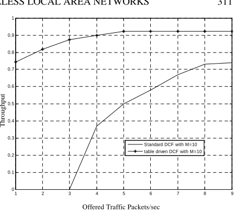
Figure 5 shows a comparison of the throughput between the table driven DCF and the standard DCF (IEEE 802.11) for 10 stations. The values of standard DCF are taken from [5] which uses the same parameters as in [4]. It is evident the table driven DCF performs better than the standard DCF (IEEE 802.11).
Figure 6 shows a comparison of average delay between the table driven DCF and the standard DCF (IEEE 802.11). The values of standard DCF are again taken from [5]. It is noticeable that the delay performances are the same.
[image:5.595.307.539.61.269.2]Figure 7 shows the throughput curve for different offered loads for the table driven RTS/CTS technique. It shows that the throughput rises and becomes saturated at higher values of the load. The maximum throughput calculated by “Bianchi” in [4] for the standard RTS/CTS (IEEE 802.11) mechanism is 0.837281 when M=10.
Figure 5. Throughput comparison between the table driven DCF and the standard DCF (IEEE 802.11).
Figure 6. Average Delay Comparison between the table driven DCF and standard DCF (IEEE 802.11).
Figure 7. Throughput corresponding to different offered traffic for table driven RTS/CTS.
1 2 3 4 5 6 7 8 9
0 0.1 0.2 0.3 0.4 0.5 0.6 0.7 0.8 0.9 1
Offered Traffic Packets/sec
[image:5.595.51.289.79.246.2] [image:5.595.307.541.304.488.2]Standard DCF with M=10 table driven DCF with M=10
T h ro u g h p u t
Offered Traffic Packets/sec
1 2 3 4 5 6 7 8 9
0 0.2 0.4 0.6 0.8 1 1.2 1.4
[image:5.595.314.537.531.722.2]Standard DCF with M=10 table driven DCF with M=10
Offered Traffic Packets/sec
A v er ag e D el ay i n S ec o n d s
1 2 3 4 5 6 7 8 9
0.8 0.82 0.84 0.86 0.88 0.9 0.92
table driven RTS/CTS
Offered Traffic λ packets/sec
500 1000 1500 2000 2500 3000 3500 1
2 3 4 5 6 7 8 9 10 11
No of Transmission Periods
T
h
ro
u
g
h
p
u
t
a
n
d
T
ra
ff
ic
(λ
)
Input Traffic λ Throughput
Figure 8. Throughput and input traffic corresponding to the number of transmission periods (table driven RTS/CTS).
From the Figure 7 it is evident that table driven RTS/CTS performs better than the standard RTS/CTS in terms of throughput.
The table driven RTS/CTS technique has an extra advantage as it is a load adaptive system. It means that it has the capability to adapt to the input traffic as quickly as possible. Figure 8 shows a case where the input traffic suddenly increases from 5 packets/sec to 10 packets/sec. In this case the throughput
(
η×Input traffic rate( )λ)
is shown to follow the offered trafficλ
.Fairness (FI) is another important issue considered in this paper. To express this, we take the fairness index defined in [10] and [2] to measure the fair packet capacity allocation. In [10] fairness index is represented as
1
1 1
1
r n
i i
n r
i i
x n
x n
=
=
∑
∑
. For example if m dollars are to be
distributed among n people and we favor k people by giving them m/k dollars each and discriminate against n-k
people, then the above function becomes
1
r k FI
n −
= .
Favoring 10% would result in a fairness index of 1
0.1r
FI = − and discriminate index of 1 0.1− r−1. Therefore
r should be equal to 2. That is,
(
)
(
)
2
1
2 1
n i i
n i i
x FI
n x
=
=
=
∑
∑
, whereFI is the fairness index, n is the number of stations,
x
iis the packets transmitted by thei
thactive station during the simulation time (current traffic in which the offered trafficλ is same for all stations).
Figure 9 shows the comparison of the fairness index performance of table driven DCF, table driven RTS/CTS and standard DCF (IEEE 802.11). It can be observed that, for the three cases up to 15 active stations the performance is fair.
Figure 9. Fairness index for different number of stations for table driven DCF, table driven RTS/CTS and standard DCF (IEEE 802.11).
6. Conclusions and Future Work
In this paper a new approach that is based on the table driven technique is proposed for DCF and RTS/CTS mechanism in WLANs. While maintaining the same delay the table driven DCF outperforms the standard DCF (IEEE 802.11) in terms of throughput. The table driven RTS/CTS also demonstrates that its throughput is more than the standard RTS/CTS mechanism. Moreover the table driven DCF and table driven RTS/CTS gives very good fairness performance. In the table driven technique (for both DCF and the RTS) a simple search mechanism is used to find the values of M and p from WL and
C
. However an efficient lookup mechanism is required for this purpose.The subnet technique presented in this paper is amenable to implementation with two hops or more from the SS (subscriber stations) of the IEEE802.16. This SS is typically aware of the number of the nodes of the subnet of the IEEE802.11 standard and will broadcast such number to the nodes of the IEEE802.11 subnet. The nodes may use this value as rule of thumb against the actual estimated value of M obtained by the new table driven technique. This current paper estimates p and M from the nodes activities on the channel. Further, the value of M from SS and its favorable consequences are for future research. Our table based technique shall hence improve the performance of such subnet.
7. References
[1] X. J. Tian, X. Chen, T. Ideguchi, and Y. G. Fang, “Improving throughput and fairness in WLANs through dynamically optimizing backoff,” IEICE Transactions on Communications 2005 E88-B(11), pp. 4328–4338.
[2] L. Zhang, Y. T. Shu, and O. Yang, “Performance improve- ment for 802.11 based wireless local area networks,”
5 6 7 8 9 10 11 12 13 14 15
0.8 0.85 0.9 0.95 1 1.05
Table driven DCF Table driven RTS Standard DCF
Number of Mobile station
F
ai
rn
es
s
In
d
IEICE Transactions on Communications, Vol. E90-B, No. 4, April 2007.
[3] V. Bharghvan, “Performance evaluation of algorithms for wireless medium access,” IEEE International Computer Performance and Dependability Symposium IPDS’98, pp. 86–95, 1998.
[4] G. Bianchi, “Performance analysis of the IEEE 802.11 distributed coordination function,” IEEE Journal of Selected Areas on Communications, Vol. 18, No. 3, pp. 535–547, March 2000.
[5] S. Pasupuleti and D. Das, “Throughput and delay evaluation of a proposed-DCF MAC protocol for WLAN,” IEEE INDIA annual conference 2004, lndicon 2004. [6] F. Cali, M. Conti, and E. Gregori, “Dynamic tuning of the
IEEE 802.11 protocol to achieve a theoretical throughput limit,” IEEE/ACM Transactions on Networking, Vol. 8, No. 6, pp. 785–799, December 2000.
[7] Y. Kwon, Y. Fang, and H. Latchman, “A novel MAC protocol with fast collision resolution for wireless LANs,” IEEE INFOCOM’03, April 2003.
[8] J. Weinmiller, H. Woesner. J. P. Ebert, and A. Wolisz, “Analyzing and tuning the distributed coordination function in the IEEE 802.11 DFWMAC draft standard,” Proceedings MASCOT, San Jose, CA, February 1996.
[9] S. Khurana, A. Kahol, S. K. S. Gupta, and P. K. Srimani, “Performance evaluation of distributed co-ordination function for IEEE 802.11 wireless LAN protocol in presence of mobile and hidden terminals,” Modeling, Analysis and Simulation of Computer and Telecommunication Systems, 1999, Proceedings, 7th International Symposium, Digital Object Identifier 10.1109/MASCOT.1999.805038, pp. 40–47, October 24–28, 1999.
[10] R. Jain, D. Chiu, and W. Hawe, “A quantitative measure of fairness and discrimination for resource allocation in shared computer systems,” Technical Report TR-301, DEC Research Report, 1984.
[11] C. L. Fullmer and J. J. Garcia-Luna-Aceves, “Complete single-channel solutions to hidden terminal problems in wireless LANs,” Communications, 1997, ICC 97 Montreal, ‘Towards the Knowledge Millenniu’, 1997 IEEE International Conference, Vol. 2, Digital Object Identifier 10.1109/ICC.1997.609856, pp. 575–579, 8–12 June 1997.