A STUDY OF ANALYTICAL AND COMPUTATIONAL APPROACHES
TO PROBLEM SOLVING IN COLLISIONLESS SYSTEMS
Jeremy Andrew Barber
A Thesis Submitted for the Degree of PhD
at the
University of St Andrews
2014
Full metadata for this item is available in
Research@StAndrews:FullText
at:
http://research-repository.st-andrews.ac.uk/
Please use this identifier to cite or link to this item:
http://hdl.handle.net/10023/6548
This item is protected by original copyright
A study of analytical and computational approaches to problem solving in collisionless systems
by
Jeremy Andrew Barber
No man should escape our universities without knowing how little he knows.
— J. Robert Oppenheimer
Submitted for the degree of Doctor of Philosophy in Astrophysics
I, Jeremy Andrew Barber, hereby certify that this thesis, which is approximately 42,000
words in length, has been written by me, and that it is the record of work carried out by
me, or principally by myself in collaboration with others as acknowledged, and that it has
not been submitted in any previous application for a higher degree.
Date Signature of candidate
I was admitted as a research student in September 2010 and as a candidate for the
degree of PhD in September 2010; the higher study of which this is a record was carried
out in the University of St Andrews between 2010 and 2014.
Date Signature of candidate
I hereby certify that the candidate has fulfilled the conditions of the Resolution and
Regulations appropriate for the degree of PhD in the University of St Andrews and that
the candidate is qualified to submit this thesis in application for that degree.
In submitting this thesis to the University of St Andrews we understand that we are giving
permission for it to be made available for use in accordance with the regulations of the
University Library for the time being in force, subject to any copyright vested in the work
not being affected thereby. We also understand that the title and the abstract will be
pub-lished, and that a copy of the work may be made and supplied to any bona fide library or
research worker, that my thesis will be electronically accessible for personal or research
use unless exempt by award of an embargo as requested below, and that the library has
the right to migrate my thesis into new electronic forms as required to ensure continued
access to the thesis. We have obtained any third-party copyright permissions that may be
required in order to allow such access and migration, or have requested the appropriate
embargo below.
The following is an agreed request by candidate and supervisor regarding the
elec-tronic publication of this thesis: Access to printed copy and elecelec-tronic publication of thesis
through the University of St Andrews.
Date Signature of candidate
I present an overview of the tools and methods of gravitational dynamics motivated by
a variety of dynamics problems. Particular focus will be given to the development of dynamic phase-space configurations as well as the and the distribution functions of
colli-sionless systems.
Chapter 1 is a short review of the descriptions of a gravitational system examining Poisson’s equations, the probability distribution of particles, and some of the most popular
model groups before working through the challenges of introducing anisotropy into a model.
Chapter 2 covers the work of Barber & Zhao (2014) which looks at the relations
be-tween quantities in collisionless systems. Analytical methods are employed to describe a model that can violate the GDSAI, a well-known result connecting the density slope to the
velocity anisotropy. We prove that this inequality cannot hold for non-separable systems and discuss the result in the context of stability theorems.
Chapter 3 discusses the background for theories of gravity beyond Newton and
Ein-stein. It covers the ‘dark sector’ of modern astrophysics, motivates the development of MOND, and looks at some small examples of these MONDian theories in practice.
Chap-ter 4 discusses how to perform detailed numerical simulations covering code methods for generating initial conditions and simulating them accurately in both Newtonian and MONDian approaches. The chapter ends with a quick look at the future of N-body codes.
Chapters 5 and 6 contain work from Barber et al. (2012) and Barber et al. (2014) which look at the recent discovery of an attractor in the phase-space of collisionless sys-tems and present a variety of results to demonstrate the robustness of the feature.
At-tempts are then made to narrow down the necessary and sufficient conditions for the effect while possible mechanisms are discussed.
Finally, the epilogue is a short discussion on how best to communicate scientific ideas
I have a lot of people that I need to thank for their help and support over the last
three-and-a-bit years.
First of all, special thanks to DD. Without you I’m not sure I’d have made it this far are at all. I owe a lot of this to you. Thank you.
Thanks to my good friends – you know who you are – for being there when I needed you the most. I owe you.
Thanks to my family for supporting me even when I didn’t get to see them for a while.
Special thanks to Hongsheng. You have the patience of a saint and have taught me so much, especially in the final stretch. I hope you can be proud of the finished product.
Thanks go out to Steen for arranging all the visits and being such a lovely host. It has
been a pleasure to work with you and I very much hope to do so again.
Thanks to Xufen for letting me pester her about codes and numerical work. Thanks also to Diana and Martin for their help when I was just starting out. It’s been great to
collaborate with you all.
Thanks to all my colleagues and friends in the department. I know I haven’t been around so much lately, but it has been a pleasure to know you all. I wish you all the very
best.
Thanks to STFC, St Andrews, and DARK. Without the funding from them I wouldn’t be here in the first place.
Declaration i
Copyright Agreement iii
Abstract v
Acknowledgements vii
1 The foundations 1
1.1 Potential density pairs in Newtonian gravity . . . 2
1.1.1 Solving Poisson’s equation for the Hernquist model . . . 4
1.2 Distribution Functions . . . 5
1.2.1 Deriving a DF with constant anisotropy . . . 8
1.2.2 Examining constant anisotropy models . . . 13
1.2.3 Osipkov-Merritt models and the Cuddeford generalisation . . . 16
1.2.4 Factors for DF positivity . . . 19
2 The General Density-Slope Anisotropy Inequality in non-separable systems 23 2.1 The inadequacy of a Jeans’ equation approach . . . 26
2.2 The Distribution Function approach . . . 31
2.2.1 Finding density . . . 32
2.2.2 Finding anisotropy . . . 33
2.2.3 Finding potential . . . 35
2.3 Understanding the system . . . 36
2.3.1 Characterising the density profile . . . 36
2.3.2 Characterising the anisotropy profile . . . 41
2.3.3 The inability to extend the GDSAI to this model . . . 42
2.4.2 H´enon Instability . . . 44
2.4.3 Radial Orbit Instability . . . 46
2.4.4 Stability dependence on L2cut . . . 47
2.5 Generalising the model . . . 50
2.6 Summary . . . 55
3 The motivation for a new gravity 57 3.1 Dark matter . . . 58
3.2 Dark energy . . . 59
3.3 Breakdowns of the current theory . . . 61
3.4 Modifications to Newtonian dynamics . . . 62
3.5 The difficulties of working in MOND . . . 64
3.6 Constructing MOND models . . . 69
3.6.1 Prolate spheroid densities . . . 70
3.6.2 Finding the velocity dispersion . . . 73
3.6.3 A simple model . . . 74
3.7 Relativistic approaches . . . 78
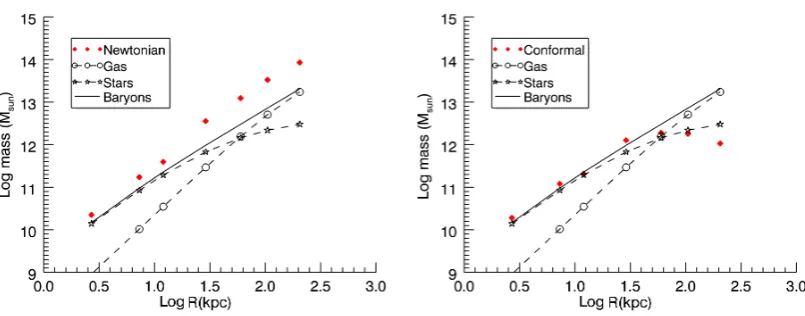
3.8 Working in conformal gravity . . . 79
4 Numerical simulation 83 4.1 Generating initial conditions . . . 84
4.2 GADGET-2: a Newtonian code . . . 86
4.2.1 Tree and TreePM force calculations . . . 87
4.2.2 Time-step determination . . . 89
4.3 NMODY: A MONDian code . . . 90
4.3.1 Force calculations and time-steps . . . 91
4.4 Hardware and next generation codes . . . 91
4.4.1 GRAPE . . . 91
4.4.2 CUDA . . . 92
4.4.3 Quantum processing . . . 95
5.2 Initial conditions and numerical code . . . 103
5.2.1 Basic perturbation . . . 105
5.2.2 Analysis pipeline . . . 107
5.3 The basic results . . . 108
5.3.1 Effect of initial anisotropy profiles . . . 110
5.3.2 Effect of gravity theory . . . 113
5.3.3 Changing implicit coordinate system . . . 116
5.3.4 Random scale factors and flow time . . . 117
5.4 Impact of numerical resolution effects . . . 120
5.5 Condensing the method — bimodal perturbation . . . 124
5.6 Connection to radial orbit instability . . . 129
5.6.1 Universal anisotropy profiles . . . 129
5.6.2 Convergence ofρ/σ3 . . . 131
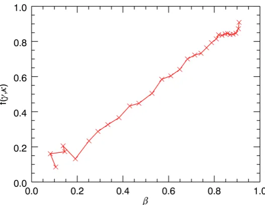
5.6.3 β -γ relation . . . 133
5.7 The story so far . . . 133
6 Necessary and Sufficient Conditions 135 6.1 Ruling out radial infall by adding energy . . . 137
6.1.1 Algorithm for avoiding infall . . . 138
6.2 The requirements for convergence . . . 140
6.2.1 Energy exchange — the anisotropy kick . . . 140
6.2.2 Energy exchange — the anisotropy contours . . . 145
6.2.3 Phase mixing in a fixed potential — the massless kick . . . 149
6.3 Impact of the attractor . . . 151
6.3.1 Density profiles . . . 154
6.3.2 Anisotropy profiles . . . 156
6.4 The path to convergence . . . 159
6.5 Summary . . . 160
7 Epilogue – communication 163 7.1 The power of analogy . . . 164
Online resources 169
1.1 DF of an anisotropic Plummer sphere . . . 13
1.2 Hernquist DFs for a set of anisotropies . . . 15
1.3 Comparison of anisotropy models . . . 18
1.4 Characteristic profiles of an anisotropic Plummer sphere . . . 20
2.1 Density of Jeans’ model for GDSAI violation . . . 29
2.2 Demonstrating the negativity of the DF . . . 31
2.3 Numerical potential from our DF . . . 37
2.4 The components of the DF density profile . . . 38
2.5 The density profile of our DF . . . 39
2.6 Angular momentum of circular orbits in our DF . . . 40
2.7 Anisotropy profile of our DF . . . 41
2.8 Radial velocity profile of our DF . . . 43
2.9 Demonstrating GDSAI violation in our DF . . . 44
2.10 H´enon instability in our DF . . . 46
2.11 ROI as a function of angular momentum threshold . . . 47
2.12 GDSAI function of our system . . . 48
2.13 LOSVD through the centre of the system . . . 50
2.14 Energy functions in the generalised DF . . . 52
2.15 Density profiles of our generalised DF . . . 53
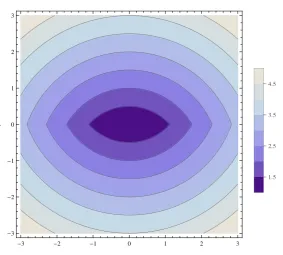
3.1 Iso-potential surfaces of a prolate system . . . 70
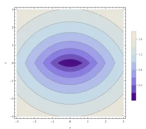
3.2 Iso-density contours for Newtonian and MOND gravity . . . 72
3.3 Iso-potential surfaces of a simple prolate system . . . 75
3.4 Iso-density contours for the simple Newtonian and MOND gravity . . . 76
5.1 The form of the attractor . . . 103
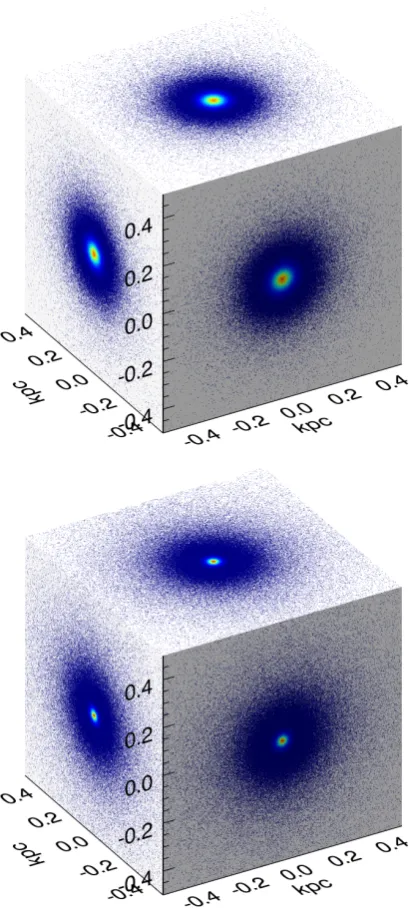
5.2 3D projection of the density . . . 109
5.3 Basic attractor evolution in a model system . . . 111
5.4 Evolution in initially anisotropic systems . . . 112
5.5 Evolution in extreme anisotropy initial conditions . . . 112
5.6 Acceleration profile showing gravitational regimes . . . 113
5.7 Evolution in weak MOND in an isotropic system . . . 114
5.8 Evolution in weak MOND in a radially anisotropic system . . . 114
5.9 Evolution in deep MOND . . . 115
5.10 The collapse of deep MOND models . . . 116
5.11 Average anisotropy contours in a stable, unperturbed system . . . 118
5.12 Anisotropy contours in a perturbed system . . . 119
5.13 Demonstrating factors effecting convergence rate . . . 120
5.14 Attractor plot demonstrating negligible two-body interaction . . . 123
5.15 Demonstration of the possible statistical roots of the attractor . . . 126
5.16 Artificial distortion of the attractor through poor algorithm choice . . . 128
5.17 Anisotropy profiles of all models . . . 130
5.18 Phase-space density profiles of all models . . . 132
6.1 Attractor plot demonstrating no radial infall . . . 140
6.2 Schematic of the anisotropy kick . . . 142
6.3 Contour plot of an isotropising kick with kick artifacts included . . . 146
6.4 Attractor plot of the same information as Fig. 6.3 . . . 146
6.5 Contour plot of a stronger isotropising kick . . . 148
6.6 Contour plot demonstrating a tangentially orientated kick . . . 148
6.7 Attractor plot of the massless kick . . . 150
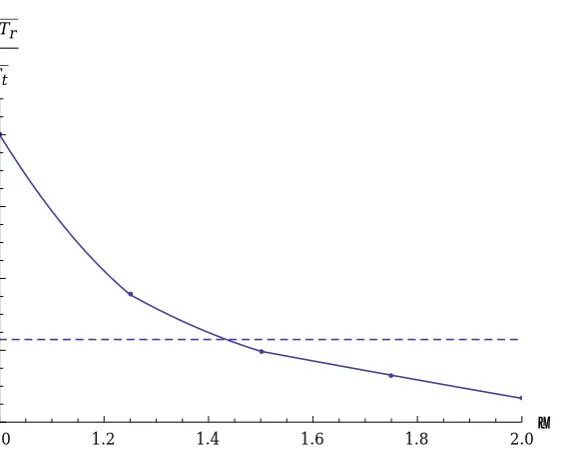
6.8 Virial ratio at the end of the flow periods . . . 151
6.9 Kinetic energy contours for the isotropic system . . . 153
6.10 Demonstrating the development of a dense nucleus and large radius envelope155 6.11 Final density profiles compared to standard profiles . . . 155
6.14 Time evolution of a single bin in phase space . . . 160
1
The foundations
“Gravity is a habit that is hard to shake off.”
— Terry Pratchett, Small Gods
It is often noted in popular physics that, among the fundamental forces in our universe,
gravity stands out as rather strange. Most obvious, perhaps, is its apparent weakness
compared to its fellows — a toy bar magnet can exert a force on, say, a paper-clip that is
many orders of magnitude more significant than the gravitational attraction of the entire
Earth. So while it is perhaps unfair to single out differences between the forces – clearly
differencesmustexist otherwise the forces wouldn’t be distinct from each other – the fact
that gravity is a good1030weaker than the other forces bears comment. It should be noted
that there is nothing ‘clear’ about how the forces are distinct from each other or, indeed,
if they even are. However that is a whole other story that will not be told in this thesis.
So, given gravity’s rather anaemic pull on matter it might be wondered, then, how
answer is what makes gravity so important. There is no such thing as negative mass.
Electrostatic forces may be born of positive or negative charge, magnets, at least generally,
have a north and a south pole, but there is no such thing as negative mass.
Why this is is a matter of debate. Nothing in fundamental physics explicitly forbids
neg-ative mass, although the properties of such material are rather counter-intuitive (Bondi,
1957). All that matters for our purposes is that the more matter that there is, the more
gravity becomes dominant. And so it is that, at galactic scales and beyond, the dynamical
behaviour and structure of the universe is governed almost exclusively by gravitational
interactions, the other forces cancelling themselves, lacking the range of transmission,
or being too specific in what they affect. Consequently, if you want to understand and
describe how anything is born, moves, evolves, and, eventually, is destroyed, gravity is
foundation of everything that you need to know.
However, this is easier said than done. Gravity can be surprisingly complex, often
confusing, and sometimes completely intractable. Therefore it is vital to have an
under-standing of the wide variety of approaches, methods, and tools that astrophysicists have
developed to solve any system that nature can conjure up (including a few that it can’t,
but are interesting anyway). On that note, let us start at the beginning and look at how
gravitational fields are born.
1.1
Potential density pairs in Newtonian gravity
At its heart, a theory of gravity describes the coupling between a distribution of matter
and an accompanying potential field. If one knows what the distribution of matter in a
system is, then the theory can be applied to predict how the matter in the system will
move. The limits on these predictions vary depending on the specifics of the theory, but
examples in Newtonian gravity include the unpredictable evolution of systems containing
more than two objects of similar mass and the degeneracy of predicted densities that can
produce a given potential (Binney & Tremaine, 2008). Newtonian gravity is the most
fa-miliar paradigm alongside its adaption into Einstein’s general relativity and between them
these theories have an imposing list of successes, ranging from predictions of gravitational
lensing to the successful launching of probes to the outer solar system.
equa-tion:
∇2Φ = 4πGρ (1.1)
In brief, this relationship is a rather neat representation of a collection ideas. A
distri-bution of matterρin some enclosed volume produces a vector field, a forceg, which can be described as the gradient of a potentialΦ. The fact that you can construct one-to-one
pairings between the potentials and the densities that created them, a level of
degener-acy aside, gives rise to the description of ‘potential-density pairs’. As powerful and as
simple as Poisson’s equation can be when dealing with complex potentials or densities
it can be difficult and time consuming to find a new solution for an unknown part of a
potential density pair. Additionally, there are certain forms of system that appear far more
frequently in nature than others, such as spheres, and having a set of well understood,
generalised potential-density pairs speeds up many areas of analysis.
This motivates a need for densities that translate easily and tractably to potentials
and vice versa but that are still accurate descriptions of physically interesting systems.
One of the earliest families used were the polytropic models (Lane, 1870). These models
were developed to describe the structure of hydrostatic, pressure supported spheres of gas
and subsequently found use in the study of stellar interiors before the advent of complex
hydrodynamic simulations. These models are a general prescription parameterised as:
1
s2 d ds
s2dψ
ds
=−3ψn;ψ >0 (1.2) where sand ψ are the dimensionless radius and positive potential. Also, much like the Dehnen models we will encounter momentarily, these are important due to their well
understood potential density pairs and relation to physical systems. One model which has
found extensive use in the field of galactic modeling, and will be appearing frequently
throughout the following chapters, is then= 5polytrope, or Plummer Sphere (Plummer, 1911).
Today, many of the most commonly useful density models are drawn from a family of
models called ‘two-power’ models after their characteristic profile of an inner power law
ρ(r) = r ρ0
a
α
(1 + ra)β−α (1.3)
Models drawn from this family thus have two free parameters besides the slope of
the power laws, a critical density, ρ0, and a scale length, a. Generically they are known as ‘two-power density laws’ but the subgroup where β = 4, the aforementioned Dehnen models (Dehnen, 1993), contain several widely used models of interest most notably the
Hernquist (Hernquist, 1990) and Jaffe (Jaffe, 1983) models having α = 1 and α = 2 respectively. To demonstrate the simple connection between the density and potential in
these models we now solve Poisson’s equation for the Hernquist model.
1.1.1 Solving Poisson’s equation for the Hernquist model
Solving a potential to find a density involves differentiation which, in almost all cases,
is an easier proposition than integration. Accordingly, we’ll do the reverse and find the
potential from the density.
The Hernquist model density profile is:
ρ(r) = M 2π
a r
1
(r+a)3 (1.4)
where a represents a characteristic length scale of the system and M is the total mass of the system. We can find the potential by first turning the density distribution into a
cumulative mass distribution. Since the volume is spherical:
M(r) =
Z 2π
0
Z π
2
−π2
Z r 0 M 2π a r 1 (r+a)3r
2sinθdrdθdφ=
−
ar
(r+a)2
r
0 −
−
a
(r+a)
r
0
(1.5)
Notice that the equations produce infinities at r=0. This can be solved by recognising
that: Z r 0 = Z ∞ 0 − Z ∞ r
andM =
Z
V
ρ(r)dV = 4π
Z ∞
0
M(r) =M−
−ar
(r+a)2
∞
r −
−a
(r+a)
∞
r
= M r
2
(r+a)2 (1.7)
From here, we can simply use the fact thatF =∇Φand thus integrate with respect to
rto find the potential:
Φ =
Z ∞
r
−GM
(r+a)2 dr=
GM r+a
∞
r
= −GM
r+a (1.8)
As useful as this is it does not contain any information on particle movements beyond
the general form of the potential. In general, dealing only with potential density pairs
makes it difficult to assess the dynamical properties of the system. What we would prefer
is a description of the system which contains information not only on particle positions,
but also contains the distribution of energy and angular momenta. To be exact, we would
like a function that describes the distribution of particles in phase-space; a ‘Distribution
Function’, so to speak.
1.2
Distribution Functions
The distribution function (DF) is a representation of a system in a six-dimensional
position-velocity phase space. At a given time the DF describes the probability of finding particles
with three-dimensional positionxand three-dimensional velocityv.
In order to understand the next chapter properly it is necessary to develop some of
the tools associated with the assessment of a DF. Most quantities derived from the DF are
found through integration and frequently require special solutions and inversions to be
analytically soluble. In order to explain them, and also to motivate the next chapter, we
will embark on a worked example of the use of a DF.
It should be noted, however, that while the DF is an incredibly simple and powerful
description of a system it generally does not do the job of relating potential to density.
The DF is just a distribution of energies and does not encode the coupling of gravitational
force like the Poisson equation does.
We can start by defining a useful quantity which describes the probability per unit
ν(x) =
Z
f(x,v)d3v (1.9)
wheref(x,v)is our DF. We can relate this to the real-space number density by multiplying by the number of stars in the system,N:
n(x) =N ν(x) (1.10)
This kind of description is particularly useful when considering how to construct
nu-merical models as it provides a natural link between the smooth density and the number
of particles used in a simulation. The DF can also immediately tell us the probability
distribution of velocities at a given position:
Px(v) =
f(x,v)
ν(x) (1.11)
wherePx(v)is the probability distribution of velocities at the pointxand can be expressed
as the probability of finding a star at x with specific velocity v over the probability of finding a star atxwithanyvelocity.
The velocity dispersion is characterised by both the changes in the mean velocity from
point to point and also the local spread of velocities around the mean at those points so
we need to find a way to describe those quantities. The mean velocity can be found by the
standard formula for expectation values:
¯ v(x) =
Z
vPx(v)d3v (1.12)
Using the expression in Eq. 1.11 we can write the mean velocity as:
¯
v(x) = 1
ν(x)
Z
vf(x,v)d3v (1.13)
Our velocity dispersion measure now has a description of the changes in mean velocity
from point to point so now we just modify it so that the spread of velocities (the variance
σ2 ≡ 1
ν(x)
Z
(v−¯v)2f(x,v)d3v (1.14) This is an analogue of the statistical measure of variance and can be expressed in a
more familiar way:
σ2= ¯v2−v¯2 (1.15)
Notice that the dispersion is governed entirely by the form of the DF. This also allows
us to define a very useful quantity which describes the ratio of energy contained within
the various axes which is the velocity anisotropy parameter:
β= 1−σ 2
θ+σ2φ
2σ2
r
(1.16)
In an isotropic system β = 0while a completely radial system gives β = 1. A com-pletely circular system gives the rather strange behaviourβ → −∞. The isotropic case is particularly important because of how it relates to the angular momentum behaviour of
the DF.
If the distribution of particles in the system is governed only by energy then the
Hamil-tonian H = K+V completely describes the motion. Accordingly we can make the
substitu-tion thatf(x,v) =v2/2 + Φin Eq. 1.13 and describe a general mean velocity.
Since this expression is a function only of v2 it is implicit that equipartition of energy will be what dictates how energy is split between the different axes. This means that the
energy will be spread evenly across all velocity components and thus all of the velocity
dispersions will be the same. In other wordsif a system has a DF that is a function only of
energy then it is necessarily isotropic.
It is easy to see why we can say that the dispersions will be equal rather than just the
mean velocities. The integral of Eq. 1.13 is over all possible velocities butvis odd while H is even. This implies that the overall integral is odd and will evaluate to0. Consequently,
¯
Having covered some of basics of the DF we can now try to use it to examine the
properties of a system we are interested in.
1.2.1 Deriving a DF with constant anisotropy
The Plummer sphere Plummer (1911) is one of the more popular models in dynamics
despite not being the most realistic thanks primarily to its considerable simplicity. Even
in this thesis Plummer spheres comprise the majority of simulations in the latter chapters
simply because of how easy they are to create with a desired anisotropy profile. Here and
now, however, we use them because we desire a simple example to illustrate two things:
how a DF can be used to create a complete system, and to show thatβis not independent of density.
We will begin with a model whose anisotropy is not a function of radius. DFs of such
systems have a simple enough parameterisation (Binney & Tremaine, 2008):
f(E, L) =L−2βf(E) (1.17)
whereLis the angular momentum distribution.
Notice that our DF is in terms of different but equivalent variables. In practice it is not
always optimal to construct a DF in terms of velocities as energies and momenta are more
fundamental descriptions. We define the relevant energies as follows:
E =−
1 2v
2+ Φ
+ Φ0 = Ψ−1 2v
2 (1.18)
whereΦ0is some constant potential andΨis the relative potentiali.e.the positive
equiv-alent of the potentialΦ.
So, we begin by finding the density of our model. Now obviously we know what this
should be because it is a well known result, but actually reproducing it is not as simple as
it might seem. Since we already know that the Plummer sphere is just the n=5 polytrope
we can save a little time and use the DF that we know leads to Plummer models. If we try
ρ=C
Z E7
2
L2β
π r2
L2
r2 +E −Ψ
−1
dL2d(−E) (1.19)
which is not conducive to analytic results. The much better way to solve this system is by
posing the question in terms of specialised coordinates. The coordinates we choose are
best at describing velocity vectors in a spherical polar system and are constructed thus:
vr =vcosη;vθ =vsinηcosχ;vφ=vsinηsinχ (1.20)
The geometry ofηandχis apparent from the consideration that forη= 0,vr =v. ηis
the angular difference between the velocity vector and the radial axis. Similarly,χ is the angle made by the velocity vector and a circumferential ring. Using this description we
can express Eq. 1.9 as:
ν=
Z
f(E, L2) d3v= 2π
Z π
0
sinηdη
Z
√
2ψ
0
v2f
ψ− 1 2v
2, rvsinη
dv (1.21)
where we applied the standard spherical volume element to arrive at this. This expression
is simple enough to integrate without further simplification to yield a general solution:
ν = 2
−(β+7/2)Cψ5−βΓ3
2−β
r2βΓ[6−β] (1.22)
C= 210π2 1(−β)!
2 −β
! (1.23)
where the gamma function is defined as (Hazewinkel, 1994):
Γ[t] =
Z ∞
0
xt−1e−xdx (1.24)
This is a rather nasty equation but for this example we do not particularly care about
the full range of its behaviour. Remember that we are just trying to find the density profile
interesting we examine the case ofβ= 1/2instead which yields:
ν = Dψ 9/2
r (1.25)
whereDis some constant. We need to be able to solve the Poisson equation now which, upon substitution, takes the form:
1
r2 d dr
r2dψ
dr
+ 4πGD rψ
9/2 = 0 (1.26)
If you think back to start of the chapter we talked briefly about how polytropes are
derived from the Lane-Emden equation (LE) of Eq. 1.2. As you can perhaps see, Eq.
1.2 can be derived directly from Eq. 1.26 with only some small assumptions about the
equations of state were it not for one problem.
The problem is that in this version there is an extra factor of r that is not normally
present. Explicitly, if we had solved for an isotropic system rather than an anisotropic one
then we would have arrived at the standard Plummer result:
ν =F ψ5 (1.27)
which leads to the LE and is one of the rare analytical solutions to it given that F is just some constant
All of this highlights the essential problem with gravitational systems and why we place
so much emphasis on potential-density pairs. It is extremely rare to find a system where
everything is simple. You can start from a simple DF but be left with a non-analytic density
or you can start from a simple potential-density pair but the DF is extremely complex.
The isotropic Plummer model is one of the simplest models around but even that rapidly
becomes obstructively complex when applying a basic anisotropy law.
The reason for the complexity is this. The anisotropy cannot be directly accounted
for in the density profile or potential i.e. if presented with a standard Plummer density
profile there is no way to tell what anisotropy behaviour it has without needing additional
information. Because of this, the anisotropy is best introduced at the level of the DF as it
However, as we have just seen, if we introduce anisotropy at the DF level we will not
recover the same density profile as an isotropic DF would have done. This is because by
changing the anisotropy at a given radius the available phase-space is smaller and thus
the real-space density is also lower.
So, this leaves us in a quandary. If we want to build an anisotropic, analytic model
we must start from the DF but then still guarantee the form of the resulting density. One
of the better ways to try and arrive at an analytical solution for a general system is to
perform an inversion.
If we go back to our general solution for the constant anisotropy model in Eq. 1.21 we
can choose not to specify the DF we were using to instead arrive at:
1 2 −β
! √
π(−β)! 2β−1/2
2π r
2βν =
Z ψ
0
f(E) (ψ− E)β−12
dE (1.28)
where we have solved the integral over η. Now this may not seem like an improvement on our first attempt, but it is saved by a standard result called the Abel integral. The Abel
integral is a useful inversion formula which we will see again later. The inversion is as
follows:
f(x) =
Z x
0
g(t)
(x−t)αdt→g(t) =
sin(πα)
π
Z t
0
dx
(t−x)1−α
df(x) dx +
f(0)
t1−α
(1.29)
This particular integral is especially useful in the mathematics of DFs because of how
often one ends up solving equations of the form:
dν
dΨ =
Z Ψ
0
f(E) √
Ψ− EdE (1.30)
where it is known as Eddington’s formula (Eddington, 1916). So, if we apply this to our
current system then we can find the troublesomef(E) section of our DF. This still isn’t simple or necessarily analytic but it is a good start. Let us once again take a case where
f(E =ψ) = 1 2π2
d
dψ(rν) (1.31)
We can solve this directly into a function of radius because we can ‘cheat’ a little bit
and simply use the Plummer potential density pair. We could solve the isotropic case to
derive it ourselves if we really wanted to but we can save ourselves a little time instead.
We know the Plummer potential-density pair is simply:
ψ= p 1
1 + (r/a)2;ν= 3 4πa3
1 +r 2
a2
−52
(1.32)
where a ≡ra. We can rearrange these relations to solve Eq. 1.31 and with that we can
arrive at our DF:
f(E) = 3 8π3a2E
3
5p1− E2−√ 1 1− E2
(1.33)
If we were to solve this DF again we would recover a standard Plummer model with
an anisotropyβ = 1/2. However, there is still a problem with the model and this time it is something more serious than just mathematical inconvenience. If we plot the form of
the DF we see that it has two main regions with different behaviour. At smaller values
of E, corresponding to larger radii, we see that the DF is always positive and gradually
increases up to some maximum value off(E). At smaller radiiE →1and what we see is thatf(E)drops very rapidly as shown in Fig. 1.1.
Of critical importance is the fact that there is no way to avoid that asr →0the model always follows f(E) → −∞ which is disastrous. Remember, at its most basic the DF represents a probability distribution and so must globally obey f(E) ≥ 0 in order to be consistent. If the DF is anywhere negative then the probability of finding a particle at that
position in phase-space cannot be meaningfully assessed and the model breaks down. In
short, global non-negativity is a primary measure of the success of a DF.
What we have found is that our model will fail in a manner that is not found in isotropic
versions of the same system as the usefulness of the isotropic Plummer sphere is well
established. Additionally we have shown that it is not possible to simply force a given
0.2 0.4 0.6 0.8 1.0 E
-0.010 -0.005 0.005 0.010fHEL
Figure 1.1: The energy function of a DF describing a Plummer sphere with a constant
β= 1/2. Note the negativity of the DF, and hence the failure of the model, at small radii.
fail and which will succeed.
What we can take from this model is that the failure occurs at low radii around the
region where a Plummer sphere is near to its constant density core. At large radii the
density drops off asr5 and the model seems to work. We may examine this relationship further if we examine a few more models and, along the way, discuss how to make a more
realistic anisotropy description.
1.2.2 Examining constant anisotropy models
The methods of the previous section can be applied to a variety of models but there is
no guarantee of whether the result will produce a viable system. Fortunately, finding
solutions for these systems has been a major endeavour which has lead to some measure
of success. For example we can now move on to examine constant anisotropy Hernquist
models.
Rather than solving the system ourselves, as we did for the Plummer model, we will
instead use the results of Baes & Dejonghe (2002) from their exhaustive examination of
the Hernquist model. They used a similar analysis routine to arrive at the DF for a constant
f(E, L) = 2
β
(2π)5/2
Γ[5−2β]
Γ[1−β]Γ[7/2−β]×L
−2βE5/2−β
2F1
5−2β,1−2β;7 2−β;E
(1.34)
where2F1is a hypergeometric series given by (Hazewinkel, 1994):
2F1(a,b;c;z) =
∞
X
n=0
(a)m(b)m
(c)m
zm
m! where(a)m=a(a+ 1)(a+ 2). . .(a+m−1) (1.35)
This is an example of how simple DFs and simple potential-density pairs tend to be
mutually exclusive. It’s a little difficult to assess the complete behaviour of this system.
However, all we really care about is the positivity of the system for a variety of anisotropies
so we can make a few assumptions to simplify it.
First of all we know that the angular momentum will always be non-negative and so
we can ignore factors of L for our analysis. Likewise, for bound particles we know that
E will always be positive as well and since the system is defined as bound we can ignore pre-factors ofE as well. Finally, we need to think about the various gamma functions.
From Eq. 1.24 we can see that none of our gamma functions will be negative for any
value ofβ so we can equate the positivity of the DF with the behaviour of the hypergeo-metric series. If we plot ourf(E) against the domain ofE we can check the positivity for a range of anisotropies.
As we can see from Fig. 1.2 we have three cases of interest. The DF is always positive
forβ ≤1/2with the additional case that, as can be seen from the thick curve in Fig. 1.2,
β = 1/2gives a constant value:
f(E, L) = 3 4π3
E2
L (1.36)
This is also the last case that retains the property of global positivity. In every other
case the DF will be negative for large values ofE which corresponds to small radii.
What we are seeing is that it is difficult to make a system with a large anisotropy when
0.2 0.4 0.6 0.8 1.0 E
-1 1 2 3
2F1@fHEL D
Figure 1.2: The hypergeometric series term for an anisotropic DF producing a Hernquist
model as a function ofE for a variety of anisotropies. The different curves for β={0,0.25,0.50,0.75}are the dotted, dashed, thick, and thin lines respectively.
to set an anisotropy that is greater than half the magnitude of the density slope.
The Plummer sphere we developed actually didn’t have a globally positive solution
that generated anisotropy in the constant density core. In the Hernquist profile, which has
a central cusp ofr−1, we cannot generate an anisotropy of more thanβ= 1/2. In fact, this result holds for all of the Dehnen models. A general DF for Dehnen models withβ = 1/2 is given by Buyle et al. (2007):
f(E, L, γ) = 3−γ 8π3L
1−(1−(2−γ)E)1/(2−γ)
2
4−γ+ γ−1
(1−(2−γ)E)1/(2−γ)
!
(1.37)
where the parameter γ chooses the slope of central cusp according to Eq. 1.3. Again, we see that the last term in this DF will force the function to be negative if γ < 1. In other words, it would appear as if the density slope and the anisotropy are bound by the
requirement that the former be at least twice as big as the latter.
To examine this in some detail we need to look at something more than just the simple
cases of constant anisotropy and to dothatwe need a more powerful method.
It should be noted that the assumption of constant anisotropy is not without its uses.
anisotropic DFs for dark matter halos using NFW and Moore profiles. However, it must
still be acknowledged that real systems tend to have more complex anisotropy profiles and
one must be cautious when extending the results from simpler models.
1.2.3 Osipkov-Merritt models and the Cuddeford generalisation
If you want to try and construct an analytical DF for a particular potential density pair
then your options are rather limited. One of the few ways to do this reliably is by using
the method of Osipkov (1979) and Merritt (1985) which is essentially an extension of the
methods that we have used so far.
In the Osipkov-Merritt formalism the energy dependence of the system is expanded to
include an angular momentum term:
f(E, L) =f(Q) =f
E − L 2
2r2
a
(1.38)
where the termrais a radius which determines the shape of the anisotropy profile.
If we make the substitution into the polar coordinate space that we used back in Eq.
1.20 then we can recover the following form of Eq. 1.21:
ν(r) = 2π
Z π
0
sinηdη
Z ψ
0
f(Q)
p
2(ψ−Q) (1 + (r/ra)2sin2η)3/2
dQ (1.39)
which inverts into a rather familiar equation:
f(Q) =√1 8π2
" Z Q
0
dψ
√
Q−ψ
d2νQ
dψ2 + 1 √
Q
dνQ
dψ
ψ=0
#
(1.40)
thanks to the striking similarity to the Abel integrals we have already been dealing with
back in Eq. 1.29. This construction has a number of nice features that spring from the
familiarity of this result not least of which is the simple relationship between the density
of these models and the isotropic model:
νQ(r) =
1 +r 2
r2
a
ν(r) (1.41)
general result for the anisotropy profile:
β(r) = 1 1 +r2
a/r2
(1.42)
This is the problem, at least for us, with Osipkov-Merritt models. The system is always
anisotropic atr = 0and will be nearly isotropic for allr rabefore smoothly becoming
more radially anisotropic for r ra. This is very good for most systems, but we are
wanting to discuss models with a central anisotropyβ0 >0. For that we need a different formalism such as the one provided by Cuddeford (1991).
In this system the Osipkov-Merritt model is extended according to:
f(E, L) =f0(Q)L−2β (1.43)
This minor alteration gives us a similar density profile:
νQ(r) =r−2β
1 +r 2
r2
a
β0−1
ν(r) (1.44)
but, importantly, yields a much more flexible anisotropy profile:
β(r) = 1 +β0r 2
a/r2
1 +r2
a/r2
(1.45)
This reduces to the Osipkov-Merritt profile for the case of β0 = 0and a comparison of the two profile shapes is given in Fig. 1.3. In particular we note that the Cuddeford
models allow the central anisotropy to be specified with the rest of the model describing
the increasing radial anisotropy.
So now we can yet again go through the process of inverting the expression for density
into one for the DF through the Abel integral to produce a generalised expression for
Cuddeford models. It is more difficult than in our simple example but with suitable choice
of variables and differentials an analogous form can be found. The principle difficulty
comes from the requirement for repeated differentiations depending on what anisotropy
0.0 0.5 1.0 1.5 2.0 2.5 3.0 r ra 0.2 0.4 0.6 0.8 1.0 Β
Figure 1.3:A comparison of the anisotropy profiles created by Osipkov-Merritt (solid) and
Cuddeford (dotted) models. The Cuddeford model usesβ0= 1/2.
f(E, L) = 2
β0
(2π)3/2
L−2β0
Γ[1−β0]Γ[1−m] d dQ
Z Q
0
dnf(E, L) dψn
dψ
(Q−ψ)m (1.46)
where we need to define a few terms to deal with the unusual amount of differentiation:
n= 1 +
1 2−β0
;m=
1 2 −β0
−
1 2 −β0
(1.47)
wheredxeis the ceiling function (Hazewinkel, 1994).
As you can perhaps appreciate this DF is very difficult to evaluate for generic values
of β0 and most treatments limit themselves to the simpler solutions for integer or half integer values as these cases are the only ones with analytical solutions. This is a slight
problem for us here as we are interested in analytical solutions where β0 >1/2but none exist. β0 = 1 is technically such a case but since the inversion is only valid for β0 < 1 (Cuddeford, 1991) we cannot use that case either.
However, an examination of the system can still give us some insights. If the anisotropy
radius is allowed to tend towards infinity then we will recover a system with constant
anisotropy which we already have tested. Additionally, allowing the anisotropy radius
to decrease will only cause the anisotropy to increase at a given radius. In other words
if a constant anisotropy system would fail to have a globally positive DF due to a high
This means that the results for our constant anisotropy Hernquist model still stand for the
Cuddeford model (Baes & Dejonghe, 2002).
1.2.4 Factors for DF positivity
The final point we will cover for this chapter is to mention that the relationship between
anisotropy and the DF is far from the be-all and end-all of DF positivity. We will discuss
this extensively in the next chapter but what we have been uncovering is an established
result stating that the anisotropy can never exceed half the logarithm of the density slope.
This relationship is outlined in Ciotti & Morganti (2010b) and is known as the general
density-slope anisotropy inequality.
That will be the focus of the next chapter but for now we will just prove that a DF
can be negative without this being due exclusively to the anisotropy. Thinking back to
the constant anisotropy Plummer model we found that, due to the constant density core,
the model cannot be radially anisotropic at small radii. Armed with only this fact and the
inequality of Ciotti & Morganti (2010b) we might perhaps expect that we can predict the
positivity of the DF.
We could, for example, assume that any Cuddeford models with β0 > 0 would have negative DFs which, for the Plummer model at least, is accurate. However, we might
suppose that Osipkov-Merritt models would be allowed due their behaviour thatβ0= 0at the centre of the system.
This has been examined in Dejonghe (1987) although with a more flexible anisotropy
profile than the Osipkov-Merritt model allows. In that paper an analytical set of solutions
was found which produced Plummer spheres with an anisotropy given by a parameter q:
β= q 2
r2
1 +r2 (1.48)
This generalisation is different to that of Cuddeford (1991) as the anisotropy at the
core is always zero like an Osipkov-Merritt model but the anisotropy radius is implicit
rather than explicit. Incidentally, the generalisation recovers an Osipkov-Merritt type
anisotropy profile for q= 2.
0.5 1.0 1.5 2.0 2.5 3.0 r
-1 1 2 3 4 5 2Β and Γ
Figure 1.4:A comparison of2βagainst the logarithmic density slope. The slope of the density
profile is the thick curve while anisotropy profiles for q= 1,3,6 are the dotted, dot-dashed, and dashed curves respectively. Note that the anisotropy curves are
2β rather thanβ for direct comparison. Curves above the density slope profile are expected to cause a negative DF.
to inversion. We have gone over the mechanics of these inversions in detail so we shall
just state the result of Dejonghe (1987). The DF to generate anisotropic Plummer spheres
is:
f(E, L) = 3Γ[6−q] 2(2π)5/2Γ[9/2−q]E
7/2−q
2F1
p/2, q−7/2; 1;L 2
2E
(1.49)
We should note that the full function is larger but we have simplified it here as we are
only interested in a very specific case. As with previous models the fact that we are only
interested in the positivity of the DF means we can neglect a large amount of the DF since
the positivity is once again entirely dependent on the behaviour of only one component.
Accordingly, as before, if we understand the positivity of the hypergeometric series then
we will understand the positivity of the DF.
But first, we can make a prediction based on our experiences of the anisotropy relation.
It is simple to plot twice the anisotropy profile against the power law of the density slope
to produce Fig. 1.4.
We can actually examine the relationship between the anisotropy and the density slope
2β = qr 2
1 +r2; d logρ
d logr =
d log d logr
3 4π(1 +r2)5/2
= 5r 2
1 +r2 (1.50)
If we set these two terms equal to each other then we can solve for the value of q
at which we would expect the change from a positive to a negative DF to occur. Doing
so gives us the simple result of q = 5. This is a rather interesting result as we should
immediately notice that a value that large will very quickly produce an anisotropy that
is physically impossible; a system that is more than twice as radial as a completely radial
system. We could take this to reasonably mean that we can set any value for the anisotropy
of these models and as long as it is physically meaningful then it will never lead to a
negative DF.
This is a very neat result and makes this system of modelling very useful for
produc-ing Plummer spheres, but we are interested in this because of what it implies about the
positivity. If the anisotropy cannot meaningfully go above β = 1 then any system that claims to do so must be non-physical. If it is non-physical then it must necessarily have a
negative DF so that the model cannot be produced. To achieve an anisotropy ofβ = 1at large radii we require q = 2which means that this value for q must be the real limit on
the DF positivity.
In other words, what we have proved is that the rule where the anisotropy cannot
exceed half the logarithmic density slope is not a necessary condition for a positive DF. It
is sufficient but there are other factors which may be of greater importance.
Now we have a robust understanding of the background to the DF formalism and have
introduced a little of the results from Ciotti & Morganti (2010b) we may now embark on
2
The General Density-Slope Anisotropy
Inequality in non-separable systems
“Everyone has an equal right to inequality.”
— John Ralston Saul
In the last chapter we covered a lot of material to do with the business of finding DFs
and solving models in order to use or plot them. In this chapter we are going to expand on
this a little more by looking at one problem in much greater detail. Throughout the latter
half of chapter 1 we ran into an apparent relationship between the density slope and the
anisotropy profile and it is that that we are going to investigate. This will obviously use a
large amount of the material that we discussed in the previous chapter so, to summarise,
the key points are as follows.
It is often difficult to derive the anisotropy of a system from observational data as the
thus extremely useful to find constraints and relationships that allow the anisotropy to be
known as a function of more easily observed variables such as density.
Usually a particular potential or density profile will be chosen to model a particular
system of interest. The most effective and powerful presentation of such a system is the
phase-space distribution function (DF) which is connected to observable, real-space
quan-tities of a system via various integral relations. Because the DF is a probability distribution
that describes the phase-space of a system there are some fundamental requirements for
a DF that produces a viable system. The most basic constraint is the positivity of the DF
over the entire permitted domain of the system as while a system with a positive DF may
not be stable, but a system with a negative DF cannot even be created.
The relationship between a density profile and a DF is complicated and is not even
one-to-one (Dejonghe, 1987). Since the DF describes the full six-dimensional shape of the
system there are multiple possible DFs that can produce the same density profile which
only differ through, for example, their anisotropy profiles. Accordingly, it is very important
to be able to derive unambiguous analytical expressions for a system of interest so that
the positivity can be known precisely.
The main problem here is that the process of finding an expression for the DF of an
arbitrary system is highly non-trivial and can usually not be done analytically. The most
reliable method of finding a DF is through Eddington’s formula (Eddington, 1916) which
inverts the integral relationship between the density and the DF, however even this is only
analytic for a selection of density profiles and parameters.
So in general, while specific models and schemes to produce analytical DFs for a given
density do exist, there is a pressing need for simple, fundamental relationships between
the quantities of a system that can constrain the positivity of a DF. A way to look at a
particular model and know, without having to work through the inversions, whether or
not the DF is likely to be positive would be ideal.
One particularly important result was that of Ciotti & Pellegrini (1992) who found a
simple criteria for the consistency of models using an Osipkov-Merritt anisotropy scheme.
This paved the way for a dramatic expansion in the scope of relations between DF
positiv-ity and anisotropy profiles, which would eventually lead to the birth of the result we will
dark halo under reasonable assumptions of spherical symmetry, a power law phase-space
density (Taylor & Navarro, 2001), and the requirement for physical solutions to the Jeans
Equations (which we will be discussing shortly). They found that any system with an
in-ner density profileρ∝r−γ would obey1 +β ≤γ ≤3where β is the velocity anisotropy
parameter.
This was subsequently improved until the relation could constrain a non-negative DF
(An & Evans, 2006) in multi-component systems (Ciotti & Morganti, 2009) and Cuddeford
models (Cuddeford, 1991; Ciotti & Morganti, 2010a) which contain the Osipkov-Merritt
models as a special case. After the discovery that the constraints held even for systems
outside these model groups (Ciotti & Morganti, 2010c) there was an effort made to define
exactly how universal such constraints could be. This lead to the significant result of Ciotti
& Morganti (2010b) where it was proven that a large class of models obey the relation:
γ ≥2β (2.1)
This relationship was termed the Global Density Slope-Anisotropy Inequality (GDSAI)
and was shown to be strongly connected to the positivity of the DF in this broad class
of multi-component models Cuddeford models as well as in a variety of other anisotropic
systems. Specifically, the work of Van Hese et al. (2011) showed that obeying the GDSAI is
a necessary condition for DF positivity in models where the central anisotropy wasβ0≤0 but did demonstrate counter-examples for larger anisotropies.
All the systems that had been investigated and had a proven relationship to the GDSAI
fall into the category of models with separable augmented density. An augmented density
is one that can be described only in terms of a potential as a function of radius and the
radius itself. A separable model of this kind can be described thusly:
ρ(r) =ρaug(ψ(r), r) =f(ψ)g(r) 0≤ψ≤ψ0 (2.2) where we alter the usual notation for the augmented density to avoid later confusion with
are referring to the density profile and are requiring the density to be expressed in two
separate functions of radius and potential. This is distinctly different from the DF being
separable and we are not interested in the separability of the DF, only the separability of
the augmented density.
Since the GDSAI has been proved for all separable augmented systems withβ0 ≤1/2 and is understood in such systems with β0 > 1/2, we will investigate the behaviour of augmented systems which are non-separable. We accomplish this by using mono-energy
DFs that produce non-separable density profiles which, while highly artificial, are also
comparatively easy to understand and analyse.
We present a simple spherical model that significantly violates the GDSAI over a range
of radii, produces systems withβ0 = 0, and has a globally positive DF. The DF is a mono-energy halo that is separable in E and L2and produces a non-separable augmented density
profile. We suggest that this is evidence that the GDSAI cannot be extended to all
non-separable systems and cannot be used to constrain the positivity of their DFs. We instead
suggest that, since our DF is not guaranteed to be dynamically stable, system stability is
still the principle measure that can confirm whether such non-separable systems can be
created and kept in equilibrium.
So, in§2.1 we briefly confirm the inadequacies of a purely Jeans Equation-based
ap-proach,§2.2 shows our construction of a simple system that does not follow the inequality,
§2.3 examines the practical implications of the system,§2.4 examines the stability of the
system,§2.5 describes possible generalisations of our model, and§2.6 concludes.
2.1
The inadequacy of a Jeans’ equation approach
It is already known that the criteria provided by the Jeans’ equations are not as stringent
as testing for the positivity of the distribution function. However, there are mathematical
difficulties associated with calculating properties of most general DFs which mean the
Jeans’ equations are still relevant. We will demonstrate why apparently simple violations
of the GDSAI which rely on the Jeans’ equations are insufficient to disprove it, as noted
in Ciotti & Morganti (2010b). This is done by creating a density profile from two simple,
superimposed models which, together, should apparently break the GDSAI according to
unphysical in a way that the Jeans’ equations cannot indicate.
First we examine the derivation of the Jeans’ equations. The Jeans’ equations are a
useful tool which can relate the observable quantities of a system which can be derived
from the DF by treating the movement of stars like the motion of a fluid. We begin from a
description of fluid flow where the change in mass contained within a surface is equated
to the flux of matter through the surface. This yields the continuity equation:
∂ρ
∂t +∇ ·(ρx˙) = 0 (2.3)
This describes the conservation of matter but can also express a conservation of
prob-ability by using the full coordinate space and the DF:
∂f
∂t +∇ ·(f [ ˙x,v˙]) = 0 (2.4)
Expanding this gives us the first step towards the Jeans’ equation:
f 3 X i=1 ∂vi ∂xi
+∂v˙i
∂vi + 3 X i=1 vi ∂f ∂xi
+ ˙vi
∂f ∂vi
= 0 (2.5)
We can eliminate some of the terms of this equation immediately. All terms of the form
∂vi/∂xican be removed as we know thatxi andvi are independent coordinates. We also
know that∂v˙i/∂vi can be removed as the acceleration is a function of∂Φ/∂xinotvi. The
result is known as the collisionless Boltzmann equation (CBE).
If we use the spherical Hamiltonian of the system we can cast our result into spherical
coordinates. Using spherical coordinates allows us to simplify the system by using
sym-metry arguments to remove angular differentials. We can also assume that the system is
time-independent which removes differentials in time. The resulting spherical CBE can
then be constructed in terms of momenta,pi, and is given by:
pr ∂f ∂r + pθ r2 ∂f ∂θ − ∂Φ ∂r − p2θ r3 −
p2φ r3sin2θ
! ∂f ∂pr −p 2 θ r2 cosθ
sin3θ ∂f ∂pθ
In order to solve this further we need to find a useful substitution for our DF. First we
should redefine our momenta in terms of the spherical coordinates used by our system:
pr = ˙r=vr;pθ =r2θ˙;pφ=r2sin2θφ˙=rsinθvφ (2.7)
which allows us to redefine the DF in terms of velocities:
Z
dprdpθdpφf =r2sinθ
Z
dvrdvθdvφf =r2sinθν (2.8)
To arrive at the Jeans’ equation from this we must multiply by a factor ofprdprdpθdpφ
and integrate. This eventually reduces to the Jeans’ equation as follows:
d(νv¯2) dr + 2
β rν
¯
v2 =−νdφ
dr (2.9)
The principle is that any system that violates this expression will be time-dependent
and thus the phase-space density will not be static. This implies that the system is evolving
and is not stable in its current configuration. This is useful for determining some of the
general properties of a system but is less descriptive than the DF.
So, the system we construct is created by overlaying a large cusped model from the
Zhao (1996) family of models onto a smaller, cored, Hernquist model (Hernquist, 1990)
to create a structure with the density profile shown in Fig. 2.1 described by:
ρ= 1
r(1 +r)3 +
5×10⁵
(7 +r)4 (2.10)
φ=−2π(7000147 + 8500042r+ 1500003r 2
3r(1 +r)(7 +r)2 (2.11)
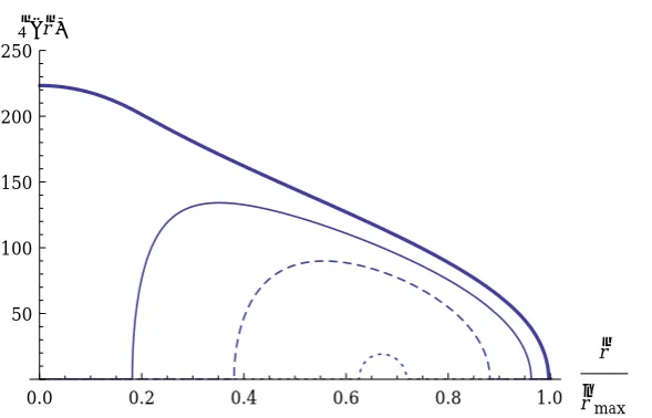
The smaller model has a cusp withρ∝r−1in the centre transitioning toρ∝r−4while the larger of the two models is cored. This means the constant density core extends past
0.001 0.01 0.1 1 10 r 5
10 50 100 500 1000 Ρ
Figure 2.1: Density profiles of a simple composite model designed to violate the GDSAI. The
dashed and dotted lines are the1/r(1 +r)3 cusped and5×105/(7 +r4)cored
subsidiary models while the solid line is the sum of the two profiles.
if we state that our system has an anisotropy ofβ = 1/2everywhere then the system will not follow the inequality.
So, we then attempt to solve the Jeans’ equation for the system:
−d(ρσ 2
r)
ρdr −
2βσr2 r =
dφ
dr (2.12)
We want to solve this forσr2so we can express this as follows assuming constantβ:
ρr2βσr2 =
Z ∞
r
ρr2βdφ
dr dr (2.13)
By definition, we can replace ddφr with terms of density instead:
ρr2βσr2 =
Z ∞
r
ρr2βG r2
Z r
0
4πr2ρdr
dr (2.14)
A full, rigorous treatment of this integral can be performed, however the density
func-tion is sufficiently complex that the analytical result is too large to be worth reproducfunc-tion
β ≥1/2then our expression will include instances of evaluating1/0 which is undefined. In other words, we cannot evaluate σr2 forβ ≥1/2meaning that any attempt to force an anisotropy which violates the GDSAI results in an unphysical solution.
The problem is that it is difficult to predict this failure in advance of solving a
spe-cific instance of the Jeans’ equation. The separate components of the model are both
independently stable, so nothing immediately seems to be wrong with the system that we
attempted to create. Rather than working through large numbers of possible models to
find combinations of parameters that work, it is easier to work directly with distribution
functions.
For instance, with the benefit of a littlea prioriknowledge, we could have known this
system would not be physical. In a system such as this we can assume that the distribution
function follows the form (Cuddeford, 1991):
f(E, L) =L−2βF(E);F(E)|E=φ=−d(rρ)
dφ (2.15)
where we assumed the form of the functionF(E)according to An & Evans (2006) assum-ing thatβ= 1/2. The problem is that the angular momentum term will always be positive but if we look at the energy term there is one region whereF(E) is locally negative. We can see this more clearly by breaking down the expression for the energy function:
F(E) =−d(rρ) dφ =−
d(rρ) dr /
dφ
dr (2.16)
To be clear, given that we need the entire energy term to be negative and
non-zero everywhere, we require d(drρr)/ddφr < 0. However, the term ddφr is always going to be positive as ddφr ≡ GMr(2<r)and clearly neither the radius nor the contained mass will be able
to become negative. The problem comes from the other term, d(drρr), i.e. the requirement
thatρmust fall steeper thanr−1.
The problem is highlighted in Fig. 2.2 where we see that rρrises for all small radii, meaning the gradient is positive. This is the region that we are interested as it contains
the transition between the two components of our model and the region in which we
0.001 0.01 0.1 1 10 r 0.001
0.01 0.1 1 10 100 1000r
Ρ
Figure 2.2: Plot ofrρ, the differential of which comprises half of the energy function of Eq.
2.16. As discussed, we require this function to have a negative gradient every-where in order for the DF to be non-negative. This figure shows that everyevery-where where the model could potentially fail to follow the GDSAI has a positive gradi-ent, indicated by the shaded areas, strongly suggesting the model is unphysical.
function Eq. 2.16 will be negative. This has the unfortunate implication that there is
a significant section of our system for which the DF is negative overall; the system is
unphysical.
In other words, the one region where we might see violation of the inequality is
un-physical by definition. If we are to investigate the GDSAI we are going to have to start
with the DF and work up, rather than the other way around.
2.2
The Distribution Function approach
We set up a system where the DF is defined as:
f(E, L) =Aδ(E−E0)H L2cut−L2
(2.17)
where the constant Ais for dimensional consistency. This represents a system where all allowed orbits have exactly energy E0and must have angular momentum L2under L2cut as
H(L2cut−L2) =
1 ifL2 < L2cut
0 ifL2 > L2cut
(2.18)
This system is actually a type of polytropic model developed by Polyachenko et al.
(2013) to study radial orbit instability. The model we use is equivalent to their q=−1
mono-energy model and is interesting to us for its non-monotonic density profile. Given
that the DF is potentially of interest, we wish to extract density and anisotropy profiles
from it to examine in detail.
2.2.1 Finding density
As we showed in chapter 1 the density is defined as the integral of the DF over all velocity
space:
ρ(r) =
Z
f(E, L) dvxdvydvz=
Z
f(E, L) dvrdvθdvφ (2.19)
To ease the subsequent integration we express the integration variables in terms of
E and L which we do by solving only for a constant radius, r. We use the following
relationships between the velocity components:
vθ2+vφ2 = L 2
r2 (2.20)
vr= √
2
r
E−Φ(r)− L 2
2r2 (2.21)
which we then use to rewrite our integration variables:
dvrdvθdvφ=
dE vr
π r2 dL
2 (2.22)
We first integrate with respect to E. This is simple as there is only one function of E,
namely vr, and the delta function makes the integration trivial. We are then just left with