A New Classifier based on The Reference Point Method with Application in Bankruptcy Prediction
Jamal Ouenniche ([email protected]) University of Edinburgh, Business School
29 Buccleuch Place, Edinburgh EH8 9JS, United Kingdom Kais Bouslah ([email protected])
University of St Andrews, School of Management,
Gateway Building, North Haugh, St Andrews KY16 9RJ, United Kingdom Jose Manuel Cabello ([email protected])
University of Malaga, Department of Applied Economics (Mathematics), Calle Ejido 6, 29071 Malaga, Spain
Francisco Ruiz ([email protected])
University of Malaga, Department of Applied Economics (Mathematics), Calle Ejido 6, 29071 Malaga, Spain
1. Introduction
Decision making under multiple and often conflicting criteria or objectives is common in a variety of real-life settings or applications. Formally, these multi-criteria problems are classified into several categories; namely, selection problems, ranking problems, sorting problems, classification problems, clustering problems, and description problems. A variety of multi-criteria decision-aid (MCDA) methodologies have been designed to address each of these problems. Ranking problems have received considerable attention in both academia and industry. One popular class of ranking methods consists of the so-called reference point methods (RPMs). To the best of our knowledge, there are no classifiers based on RPMs. In this paper, we extend the risk analytics toolbox by proposing a first RPM-based classifier and test its performance in risk class prediction with application in bankruptcy prediction.
have been studied in Ogryczak (2001). Some of the above-mentioned functions have been used in a variety of applications. Examples include paper industry (Diaz-Balteiro et al., 2011), tourism industry (Blancas et al., 2010), finance industry (Cabello et al., 2014), sustainability of municipalities (Ruiz et al., 2011), wood manufacturing industry (Voces et al., 2012), computer networks (Granat and Guerriero, 2003), procurement auctions (Kozlowski and Ogryczak, 2011), and inventory management (Ogryczak et al., 2013).
The remainder of this paper unfolds as follows. In section 2, we provide a detailed description of the proposed integrated in-sample and out-of-sample framework for RPM classifiers and discuss implementation decisions. In section 3, we empirically test the performance of the proposed framework in bankruptcy prediction of companies listed on the London Stock Exchange (LSE) and report on our findings. Finally, section 4 concludes the paper.
2. An Integrated Framework for Designing and Implementing Reference Point
Method-based Classifiers
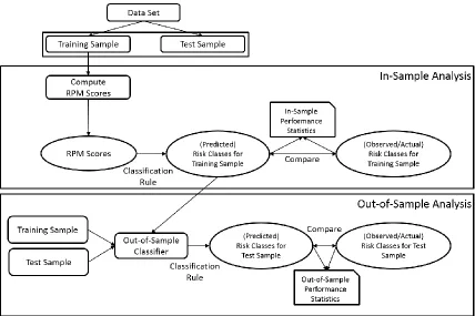
Nowadays, prediction models – whether designed for predicting a continuous variable (e.g., the level or volatility of the price of a strategic commodity such as crude oil) or a discrete one (e.g., risk class belonging of companies listed on a stock exchange) – have to be implemented both in-sample and out-of-in-sample to assess their ability to reproduce or forecast the response variable in the training sample and to forecast the response variable in the test sample, respectively. In principle, a properly designed prediction model fitted to in-sample data should be able to reproduce or predict the response variable with a high level of accuracy. However, in real-life settings, in-sample performance is not enough to qualify a prediction model for actual use in predicting the future. Because the future is unknown, out-of-sample implementation and evaluation frameworks are required to simulate the future. Therefore, an integrated framework for implementing a full classification analysis based on a reference point method; namely, in-sample classification and out-of-sample classification, is proposed in this paper.
Figure 1: Generic Design of In-Sample and Out-of-Sample Analyses of RPM Classifiers For illustration purposes, we shall customize the presentation of the proposed framework to a bankruptcy application where we reproduce or rework a classical bankruptcy prediction model; namely, the multivariate discriminant analysis (MDA) model of Taffler (1984), within a RPM classifier framework.
sample observations be denoted by 𝑥𝑖𝑗𝑘𝐸 , 𝑖 = 1, … , #𝑋𝐸, 𝑘 = 1, … , 𝑛𝑐, 𝑗 = 1, … , #𝐶𝑘 (respectively, 𝑥𝑖𝑗𝑘𝑇 , 𝑖 = 1, … , #𝑋𝑇, 𝑘 = 1, … , 𝑛𝑐, 𝑗 = 1, … , #𝐶𝑘), where #𝑋𝐸 (respectively, #𝑋𝑇) denote the cardinality of the training (respectively, test) sample and #𝐶
𝑘 denotes the cardinality of the 𝑘th category of performance criteria 𝐶𝑘.
Phase 1: In-Sample Analysis
Step 1: Choice and Computation of Double Reference Points or Benchmarks
Choose the approach and method according to which double reference points (reservation, aspiration) or virtual benchmarks, say 𝑟− and 𝑟+, are determined and compute them for each criterion or measure 𝑗 (𝑗 = 1, … , 𝑚). There are several approaches to setting up these reference points; namely, the neutral scheme where, for example, all aspiration and reservation levels are chosen as percentages of criteria ranges; the statistical scheme is based on some statistical measures of each criterion; and the voting scheme, which requires input from a group of decision makers, experts, or stakeholders – for details on these schema, see Wierzbicki et al (2000). In our risk application, we have chosen the so-called statistical scheme to show the merit of the proposed classifier empirically. Note that the use of neutral or statistical reference points results in a final comparative measure, whereas the use of the voting scheme results in an absolute measure. When the size of the training set is large enough, it seems reasonable to assume that a comparative measure is enough, and we do not need to add subjective reference points to the model. Within the statistical scheme, the best, the worst, and the average observed measure of each criterion 𝑗 (𝑗 = 1, … , 𝑚), say 𝑟𝑗𝑏𝑒𝑠𝑡, 𝑟
𝑗𝑤𝑜𝑟𝑠𝑡 and 𝑟𝑗𝑎𝑣𝑒𝑟𝑎𝑔𝑒 respectively, are first computed. Then, the double reference points (reservation, aspiration), 𝑟− and 𝑟+, are computed as follows:
𝑟𝑗− = 𝑟
𝑗𝑎𝑣𝑒𝑟𝑎𝑔𝑒−
(𝑟𝑗𝑎𝑣𝑒𝑟𝑎𝑔𝑒−𝑟𝑗𝑤𝑜𝑟𝑠𝑡)
2 ; 𝑗 = 1, … , 𝑚 𝑟𝑗+ = 𝑟
𝑗𝑎𝑣𝑒𝑟𝑎𝑔𝑒+
(𝑟𝑗𝑏𝑒𝑠𝑡−𝑟𝑗𝑎𝑣𝑒𝑟𝑎𝑔𝑒)
2 ; 𝑗 = 1, … , 𝑚 where
𝑟𝑗𝑏𝑒𝑠𝑡 = { min 𝑖=1,…,#𝑋𝐸𝑥𝑖𝑗𝑘
𝐸 𝐼𝐹𝑗 ∈ 𝑀−
max 𝑖=1,…,#𝑋𝐸𝑥𝑖𝑗𝑘
𝑟𝑗𝑤𝑜𝑟𝑠𝑡= { max 𝑖=1,…,#𝑋𝐸𝑥𝑖𝑗𝑘
𝐸 𝐼𝐹𝑗 ∈ 𝑀−
min 𝑖=1,…,#𝑋𝐸𝑥𝑖𝑗𝑘
𝐸 𝐼𝐹𝑗 ∈ 𝑀+ ; 𝑗 = 1, … , 𝑚 𝑟𝑗𝑎𝑣𝑒𝑟𝑎𝑔𝑒 = #𝑋1𝐸∑#𝑋𝑖=1𝐸𝑥𝑖𝑗𝑘𝐸 ; 𝑗 = 1, … , 𝑚
Notice that, for each criterion or its measure, the reservation reference point 𝑟𝑗− is placed half way between the worst and the average observed values of the measure, and the aspiration reference point 𝑟𝑗+ is placed half way between the average and the best values of the measure. Note that one might, in principle, choose to use a single reference point. However, from an application perspective, individual achievement functions have mainly been designed for the double reference point method. As will be seen in the next step, these functions are crucial for operationalizing these methods. Note that a major advantage of using two reference points is that they allow one to take account of the whole range of data or its distribution better than a single reference point and are likely to enhance the predictive performance of an RPM classifier.
Step 2: Choice and Computation of Each Category of Criteria-dependent Performance
Scores
For each entity 𝑖 (𝑖 = 1, … , 𝑛) and each category of performance criteria 𝐶𝑘 (𝑘 = 1, … , 𝑛𝑐), compute the strong or non-compensating performance score, say 𝑆𝑖𝑘𝑠𝑡𝑟𝑜𝑛𝑔, which does not allow for any compensation between criteria, as follows:
𝑆𝑖𝑘𝑠𝑡𝑟𝑜𝑛𝑔 = min
𝑗∈𝐶𝑘{𝑎𝑖𝑗𝑘(𝑥𝑖𝑗𝑘
𝐸 , 𝑟
𝑗−, 𝑟𝑗+)},
compute the weak or compensating performance score, say 𝑆𝑖𝑘𝑤𝑒𝑎𝑘, which allows for full compensation between criteria, as follows:
𝑆𝑖𝑘𝑤𝑒𝑎𝑘 = #𝐶1
𝑘∑ 𝑎𝑖𝑗𝑘(𝑥𝑖𝑗𝑘
𝐸 , 𝑟 𝑗−, 𝑟𝑗+) #𝐶𝑘
𝑗=1 ,
and compute the entity 𝑖 individual achievement function, 𝑎𝑖𝑗𝑘(𝑥𝑖𝑗𝑘𝐸 , 𝑟𝑗−, 𝑟𝑗+), on criterion 𝑗 with respect to the benchmarks or reference points 𝑟𝑗− and 𝑟
𝑎𝑖𝑗𝑘(𝑥𝑖𝑗𝑘𝐸 , 𝑟
𝑗−, 𝑟𝑗+) =
{
1 + 𝑥𝑖𝑗𝑘𝐸 − 𝑟𝑗+ 𝑟𝑗𝑏𝑒𝑠𝑡− 𝑟
𝑗+
, 𝐼𝐹𝑟𝑗+ ≤ 𝑥
𝑖𝑗𝑘𝐸 ≤ 𝑟𝑗𝑏𝑒𝑠𝑡
𝑥𝑖𝑗𝑘
𝐸 − 𝑟 𝑗− 𝑟𝑗+− 𝑟
𝑗−
, 𝐼𝐹𝑟𝑗− ≤ 𝑥
𝑖𝑗𝑘𝐸 < 𝑟𝑗+
𝑥𝑖𝑗𝑘
𝐸 − 𝑟 𝑗− 𝑟𝑗−− 𝑟
𝑗𝑤𝑜𝑟𝑠𝑡
, 𝐼𝐹𝑟𝑗𝑤𝑜𝑟𝑠𝑡≤ 𝑥𝑖𝑗𝑘𝐸 < 𝑟𝑗−
Note that this achievement function takes values between −1 and 2. To be more specific, when entity 𝑖 performance on criterion 𝑗 is below the reservation level 𝑟𝑗−, 𝑎
𝑖𝑗𝑘(𝑥𝑖𝑗𝑘𝐸 , 𝑟𝑗−, 𝑟𝑗+) takes values between −1 and 0; when entity 𝑖 performance on criterion 𝑗 is between the reservation level 𝑟𝑗−and the aspiration level 𝑟
𝑗+, 𝑎𝑖𝑗𝑘(𝑥𝑖𝑗𝑘𝐸 , 𝑟𝑗−, 𝑟𝑗+) takes values between 0 and 1; and when entity 𝑖 performance on criterion 𝑗 is above the aspiration level 𝑟𝑗+, 𝑎𝑖𝑗𝑘(𝑥𝑖𝑗𝑘𝐸 , 𝑟𝑗−, 𝑟𝑗+) takes values between 1 and 2. Note also that higher values of 𝑆𝑖𝑘𝑤𝑒𝑎𝑘 and 𝑆𝑖𝑘𝑠𝑡𝑟𝑜𝑛𝑔 indicate better performance.
Step 3: Choice and Computation of Overall Performance Scores
Choose a weighting scheme for the 𝑛𝑐 categories of criteria, which reflects their relative importance for the decision maker, say 𝜇, so that ∑𝑛𝑐 𝜇𝑘
𝑘=1 = 1. For each entity 𝑖 (𝑖 = 1, … , 𝑛), aggregate each of the category of criteria-dependent performance scores computed in the previous step into a single one as a convex combination of the weighted sum across categories of weak performance scores and the maximum across categories of weighted strong performance scores, commonly referred to as the mixed performance score, 𝑆𝑖𝑘𝑚𝑖𝑥𝑒𝑑 as follows:
𝑆𝑖𝑚𝑖𝑥𝑒𝑑 = 𝛼 ∑ 𝜇
𝑘𝑆𝑖𝑘𝑤𝑒𝑎𝑘 𝑛𝑐
𝑘=1 +(1 − 𝛼) min𝑘=1, …,𝑛𝑐{𝜇𝑘𝑆𝑖𝑘𝑠𝑡𝑟𝑜𝑛𝑔}; (0 ≤ 𝛼 ≤ 1).
Step 4: Use the mixed performance scores computed in the previous step to classify entities in the training sample 𝑋𝐸 according to a user-specified classification rule into risk classes, say 𝑌̂𝐸. Then, compare the RPM-based classification of entities in 𝑋𝐸 into risk classes (i.e., the predicted risk classes 𝑌̂𝐸) with the observed risk classes 𝑌𝐸 of entities in the training sample, and compute the relevant in-sample performance statistics. The choice of a decision rule for classification depends on the nature of the classification problem; that is, a two-class problem or a multi-class problem. In this paper, we are concerned with a two-class problem; therefore, we shall provide a solution that is suitable for these problems. In fact, we propose a RPM score-based cut-off point procedure to classify entities in 𝑋𝐸. The proposed procedure involves solving an optimization problem whereby the RPM score-based cut-off point, say 𝜌, is determined so as to optimize a given classification performance measure, say 𝜋 (e.g., Type I error, Type II error, Sensitivity, Specificity), over an interval with a lower bound, say 𝜌𝐿𝐵, equal to the smallest RPM score of entities in 𝑋𝐸 and an upper bound, say 𝜌𝑈𝐵, equal to the largest RPM score of entities in 𝑋𝐸. Any derivative-free unidimensional search procedure could be used to compute the optimal cut-off score, say 𝜌∗ – for details on derivative-free unidimensional search procedures, the reader is referred to Bazaraa et al. (2006). The optimal cut-off score 𝜌∗ is used to classify observations in 𝑋
𝐸 into two classes; namely, bankrupt and non-bankrupt firms. To be more specific, the predicted risk classes 𝑌̂𝐸 is determined so that firms with RPM scores less than 𝜌∗ are assigned to a bankruptcy class and those with RPM scores greater than or equal to 𝜌∗ are assigned to a non-bankruptcy class. Note that a novel feature of the design of our RPM score-based cut-off point procedure for classification lies in the determination of a cut-off score so as to optimise a specific performance measure of the classifier.
Phase 2: Out-of-Sample Analysis
class belonging for an entity 𝑖 ∈ 𝑋𝑇, because the performance of entity 𝑖 on some criterion 𝑗 might be better (respectively, worse) than 𝑟𝑗𝑏𝑒𝑠𝑡 (respectively, 𝑟𝑗𝑤𝑜𝑟𝑠𝑡) which would make the reference points inappropriate; instead, we propose an instance of case-based reasoning; namely, the k-nearest neighbour (k-NN) algorithm, which could be described as follows: Initialization Step
Choose the Case Base as 𝑋𝐸 and the Query Set as 𝑋𝑇;
Choose a distance metric 𝑑𝑘−𝑁𝑁 to use for computing distances between entities. In our implementation, we tested several choices amongst the following: Euclidean, Cityblock, and Mahalanobis;
Choose a classification criterion. In our implementation, we opted for the most commonly used one; that is, the majority vote;
Iterative Step
// Compute distances between queries and cases FOR 𝑖1 = 1 to |𝑋𝑇| {
FOR 𝑖2 = 1 to |𝑋𝐸| {
Compute 𝑑𝑘−𝑁𝑁(𝑒𝑛𝑡𝑖𝑡𝑦𝑖1, 𝑒𝑛𝑡𝑖𝑡𝑦𝑖2); }}
// Sort cases in ascending order of their distances to queries and classify queries FOR 𝑖1 = 1 to |𝑋𝑇| {
Sort the list 𝐿𝑖1 = {(𝑖2, 𝑑𝑘−𝑁𝑁(𝑒𝑛𝑡𝑖𝑡𝑦𝑖1, 𝑒𝑛𝑡𝑖𝑡𝑦𝑖2)) ; 𝑖2 = 1, … |𝑋𝐸|} in ascending order of distances and use the first 𝑘 entries in the list 𝐿𝑖1(1: 𝑘, . ) to classify 𝑒𝑛𝑡𝑖𝑡𝑦𝑖1 according to
the chosen criterion; that is, the majority vote; }
Output: In-sample and out-of-sample classifications or risk class belongings of entities along with the corresponding performance statistics.
Finally, we would like to stress out that, when the decision maker is not confident enough to provide a value for 𝛼 in step 3 above, one could automate the choice of 𝛼. In fact, an optimal value of 𝛼 with respect to a specific performance measure (e.g., Type 1 error, Type 2 error, Sensitivity, or specificity) to be optimized either in-sample or out-of-sample could be obtained by using a derivative-free unidimensional search procedure, which calls either a procedure that consists of step 1 through step 4 to optimize in-sample performance, or the whole procedure; that is, step 1 through step 5, to optimize out-of-sample performance.
In the next section, we shall report on our empirical evaluation of the proposed framework. 3. Empirical Results
Stock Exchange (LSE) during 2010-2014 excluding financial firms and utilities as well as those firms with less than 5 months lag between the reporting date and the fiscal year. The source of our sample is DataStream. The list of bankrupt firms is however compiled from London Share Price Database (LSPD) – codes 16 (Receivership), 20 (in Administration) and 21 (Cancelled and Assumed valueless). Information on our dataset composition is summarised in Table 1. As to the selection of the training sample and the test sample, we have chosen the size of the training sample to be twice the size of the test sample. The selection of observations was done with random sampling without replacement to ensure that both the training sample and the test sample have the same proportions of bankrupt and non-bankrupt firms. A total of thirty pairs of training sample-test sample were generated.
Observations (2010-2014) Nb. %
[image:10.612.164.451.286.359.2]Bankrupt Firm-Year Observations 407 6.16% Non-Bankrupt Firm-Year Observations 6198 94.38% Total Firm-Year Observations 6605 100%
Table 1: Dataset Composition
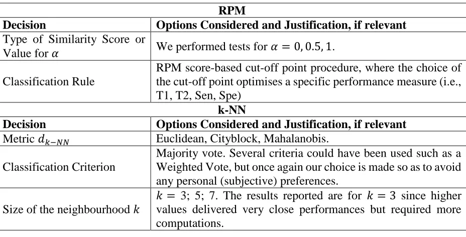
Since both the RPM classifier and the k-NN classifier, trained on the classification done with RPM, require a number of decisions to be made for their implementation, we considered several combinations of decisions to find out about the extent to which the performance of the proposed framework is sensitive or robust to these decisions. Recall that, for the RPM classifier, the analyst must choose (1) the type of similarity score to use or equivalently a value for 𝛼, and (2) the classification rule. On the other hand, for the k-NN classifier, the analyst must choose (1) the metric to use for computing distances between entities, 𝑑𝑘−𝑁𝑁, (2) the classification criterion, and (3) the size of the neighbourhood 𝑘. Our choices for these decisions are summarised in Table 2.
RPM
Decision Options Considered and Justification, if relevant Type of Similarity Score or
Value for 𝛼 We performed tests for 𝛼 = 0, 0.5, 1. Classification Rule
RPM score-based cut-off point procedure, where the choice of the cut-off point optimises a specific performance measure (i.e., T1, T2, Sen, Spe)
k-NN
Decision Options Considered and Justification, if relevant Metric 𝑑𝑘−𝑁𝑁 Euclidean, Cityblock, Mahalanobis.
Classification Criterion
Majority vote. Several criteria could have been used such as a Weighted Vote, but once again our choice is made so as to avoid any personal (subjective) preferences.
[image:11.612.75.539.242.478.2]Size of the neighbourhood 𝑘 𝑘 = 3; 5; 7. The results reported are for values delivered very close performances but required more 𝑘 = 3 since higher computations.
Table 2: Implementation Decisions for RPM and k-NN
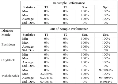
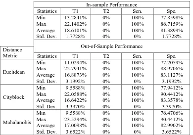
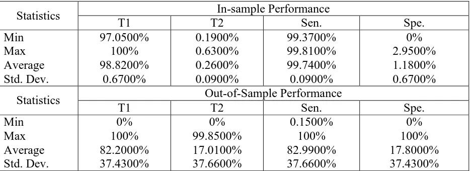
obtained with 𝛼 = 0.5; that is, when the mixed performance score is used for classification – see Table 4. As to the predictive performance of the proposed classifier when using the strong or non-compensating performance score (i.e., 𝛼 = 0), it is lower than the ones obtained with the weak and the mixed scores – see Table 5. This lower performance is expected, as the strong scheme is a much stricter one in that it only identifies the worst performance of each unit. Therefore, as far as bankruptcy prediction is concerned, we recommend the implementation of our framework using the weak performance score as long as the relevant stakeholders are comfortable with a full compensation scheme; otherwise the mixed performance score should be used with 𝛼 values closer to 1 than to 0. Note that, in risk class prediction applications, a mixed scheme may help to identify risky units that otherwise would not have been identified by a purely weak one. Note, however, that regardless of the choice of the decision maker with regards the compensation scheme, the predictive performance of the proposed classification framework is by far superior to the predictive performance of multivariate discriminant analysis – see Table 6.
In-sample Performance
Statistics T1 T2 Sen. Spe.
Min Max Average Std. Dev. 0% 0% 0% 0% 0% 0% 0% 0% 100% 100% 100% 0% 100% 100% 100% 0% Out-of-Sample Performance Distance
Metric Statistics T1 T2 Sen. Spe.
[image:12.612.115.500.372.647.2]Euclidean Min Max Average Std. Dev. 0% 0% 0% 0% 0% 0% 0% 0% 100% 100% 100% 0% 100% 100% 100% 0% Cityblock Min Max Average Std. Dev. 0% 0% 0% 0% 0% 0% 0% 0% 100% 100% 100% 0% 100% 100% 100% 0% Mahalanobis Min Max Average Std. Dev. 0% 2.2059% 0.2941% 0.4961% 0% 0% 0% 0% 100% 100% 100% 0% 97.7941% 100% 99.7059% 0.4961%
In-sample Performance
Statistics T1 T2 Sen. Spe.
Min Max Average Std. Dev. 0% 0% 0% 0% 0% 0% 0% 0% 100% 100% 100% 0% 100% 100% 100% 0% Out-of-Sample Performance Distance
Metric Statistics T1 T2 Sen. Spe.
[image:13.612.114.500.68.342.2]Euclidean Min Max Average Std. Dev. 0% 0% 0% 0% 0% 0% 0% 0% 100% 100% 100% 0% 100% 100% 100% 0% Cityblock Min Max Average Std. Dev. 0% 0% 0% 0% 0% 0% 0% 0% 100% 100% 100% 0% 100% 100% 100% 0% Mahalanobis Min Max Average Std. Dev. 0% 2.2059% 0.2941% 0.4961% 0% 0% 0% 0% 100% 100% 100% 0% 97.7941% 100% 99.7059% 0.4961%
Table 4: Summary Statistics of The Performance of The Proposed Framework for 𝛼 = 0.5
In-sample Performance
Statistics T1 T2 Sen. Spe.
Min Max Average Std. Dev. 13.2841% 22.1402% 18.6101% 1.7728% 0% 0% 0% 0% 100% 100% 100% 0% 77.8598% 86.7159% 81.3899% 1.7728% Out-of-Sample Performance Distance
Metric Statistics T1 T2 Sen. Spe.
Euclidean Min Max Average Std. Dev. 11.0294% 22.7941% 16.8873% 3.1992% 0% 0% 0% 0% 100% 100% 100% 0% 77.2059% 88.9706% 83.1127% 3.1992% Cityblock Min Max Average Std. Dev. 9.5588% 22.0588% 16.6422% 3.3970% 0% 0% 0% 0% 100% 100% 100% 0% 77.9412% 90.4412% 83.3578% 3.3970% Mahalanobis Min Max Average Std. Dev. 9.5588% 23.5294% 17.0098% 3.6522% 0% 0% 0% 0% 100% 100% 100% 0% 76.4706% 90.4412% 82.9902% 3.6522%
[image:13.612.114.504.400.673.2]Statistics In-sample Performance
T1 T2 Sen. Spe.
Min Max Average Std. Dev.
97.0500% 100% 98.8200%
0.6700%
0.1900% 0.6300% 0.2600% 0.0900%
99.3700% 99.8100% 99.7400% 0.0900%
0% 2.9500% 1.1800% 0.6700%
Statistics Out-of-Sample Performance
T1 T2 Sen. Spe.
Min Max Average Std. Dev.
0% 100% 82.2000% 37.4300%
0% 99.8500% 17.0100% 37.6600%
0.1500% 100% 82.9900% 37.6600%
[image:14.612.74.541.71.241.2]0% 100% 17.8000% 37.4300% Table 6: Summary Statistics of The Performance of MDA
4. Conclusions
References
Bazaraa, M.S., Sherali, H.D. and Shetty, C.M. (2006). Nonlinear Programming: Theory and Algorithms. (3rd edition), New Jersey: John Wiley & Sons Inc.
Benayoun, R., de Montgolfier, J., Tergny, J. and Laritchev, O. (1971). Linear Programming with Multiple Objective Functions: Step method (STEM). Mathematical Programming, 1: 366-375. Blancas, F., Caballero, R., González, M., Lozano-Oyola, M. and Pérez, F. (2010). Goal programming synthetic indicators: an application for sustainable tourism in Andalusian coastal countries. Ecological Indicators, 69: 2158-2172.
Buchanan, J. (1997). A naive approach for solving MCDM problems: The GUESS method. Journal
of the Operational Research Society, 48: 202-206.
Cabello, J., Ruiz, F., Pérez-Gladish, B. and Méndez-Rodríguez, P. (2014). Synthetic indicators of mutual funds' environmental responsibility: An application of the reference point method. European
Journal of Operational Research, 236: 313-325.
Diaz-Balteiro, L., Voces, R. and Romero, C. (2011). Making sustainability rankings using compromise programming. An application to European paper industry. Silva Fennica, 45(4): 761-773.
Granat, J. and Guerriero, F. (2003). The interactive analysis of the multicriteria shortest path problem by the reference point method. European Journal of Operational Research, 151: 103-118.
Kozlowski, B. and Ogryczak, W. (2011). On ordered weighted reference point model for multiattribute procurement auctions, in Computational Collective Intelligence. Technologies and Applications, eds. P. Jedrzejowicz, N. Nguyen and K. Hoang, Lecture Notes in Computer Science, 6922, 294-303. Springer, Berlin.
Lewandowski, A. and Wierzbicki, A.P. (Eds.) (1989). Aspiration Based Decision Support Systems. Theory, Software and Applications. Lecture Notes in Economics and Mathematical Systems, 331. Springer, Berlin.
Miettinen, K. and Mäkelä, M.M. (1995). Interactive bundle-based method for nondifferentiable multiobjective optimization: NIMBUS. Optimization, 34: 231-246.
Miettinen K. and Mäkelä M.M. (2002). On scalarizing functions in multiobjective optimization. OR
Spectrum, 24: 193–213.
Miettinen, K. (1999). Nonlinear Multiobjective Optimization. Kluwer, Boston.
Ogryczak, W. and Lahoda, S. (1992). Aspiration/reservation-based decision support – a step beyond goal programming. Journal of Multi-Criteria Decision Analysis, 1: 101-117.
Ogryczak, W., Studzinski, K. and Zorychta, K. (1992). DINAS: A computer-assisted analysis system for multiobjective transshipment problems with facility location. Computers and
Operations Research, 19, 637-647.
Ogryczak, W. (2001). On goal programming formulations of the reference point method. Journal of
the Operational Research Society, 52: 691-698.
Ogryczak, W., Perny, P. and Weng, P. (2013). A compromise programming approach to multiobjective markov decision processes. International Journal of Information Technology &
Decision Making, 12, 1021-1053.
Ouenniche J. and Tone K. (2017), An Out-of-Sample Evaluation Framework for DEA with Application in Bankruptcy Prediction, Annals of Operations Research, doi:10.1007/s10479-017-2431-5
Rodríguez-Uría, M., Caballero, R., Ruiz, F., and Romero, C. (2002). Meta-Goal Programming.
European Journal of Operational Research, 136: 422-429.
Romero, C. (1991). Handbook of Critical Issues in Goal Programming. Pergamon Press, Oxford. Romero, C. (2001). Extended lexicographic goal programming: A unifying approach. Omega. The
International Journal of Management Science, 29: 63-71.
Ruiz, F., Luque, M., Miguel, F. and Munoz, M.D.M. (2008). An additive achievement scalarizing function for multiobjective programming problems. European Journal of Operational Research, 188: 683–694.
Ruiz, F., Luque, M. and Cabello, J. M. (2009). A classification of the weighting schemes in reference point procedures for multiobjective programming. Journal of the Operational Research Society, 60: 544-553.
Ruiz, F., Cabello, J. M. and Luque, M. (2011). An application of reference point techniques to the calculation of synthetic sustainability indicators. Journal of the Operational Research Society, 62: 189-197.
Steuer, R.E. and Choo, E.U. (1983). An interactive weighted Tchebycheff procedure for multiple objective programming. Mathematical Programming, 26: 326-344.
Steuer, R.E. (1986). Multiple Criteria Optimization. Theory, Computation & Applications. Wiley, New York.
Taffler, R.J. (1984). Empirical models for the monitoring of UK corporations. Journal of Banking
and Finance, 8(2), 199–227.
Voces, R., Diaz-Balteiro, L. and Romero, C. (2012). Characterization and explanation of the sustainability of the European wood manufacturing industries: A quantitative approach. Expert
Wierzbicki, A. P. (1979). A Methodological Guide to Multiobjective Optimization. IIASA Working Paper, WP-79-122, Laxenburg, Austria.
Wierzbicki, A. P. (1980). The use of reference objectives in multiobjective optimization. In G. Fandel and T. Gal, editors, Lecture Notes in Economics and Mathematical Systems, vol. 177, pp. 468-486, Springer-Verlag, Berlin.
Wierzbicki, A. P., Makowski, M. and Wessels, J., (Eds.) (2000). Model-Based Decision Support