Stochastic Dynamics of Cholera Epidemic Model: Formulation, Analysis and Numerical Simulation

(1)

ISSN Online: 2327-4379 ISSN Print: 2327-4352

DOI: 10.4236/jamp.2019.75074 May 23, 2019 1097 Journal of Applied Mathematics and Physics

Stochastic Dynamics of Cholera Epidemic Model:

Formulation, Analysis and Numerical

Simulation

Yohana Maiga Marwa

1,2*

_{, Isambi Sailon Mbalawata}

3

_{, Samuel Mwalili}

4

_{, Wilson Mahera Charles}

5

1_{Mathematics and Statistics Department, Institute for Basic Sciences, Technology and Innovation, Pan African University,} Nairobi, Kenya

2_{Tanzania Public Service College, Singida, Tanzania}

3_{African Institute for Mathematical Sciences, Dar es Salaam, Tanzania} 4_{Jomo Kenyatta University of Agriculture and Technology, Nairobi, Kenya} 5_{University of Dar es Salaam, Dar es Salaam, Tanzania}

Abstract

In this paper, we describe the two different stochastic differential equations representing cholera dynamics. The first stochastic differential equation is formulated by introducing the stochasticity to deterministic model by para-metric perturbation technique which is a standard technique in stochastic modeling and the second stochastic differential equation is formulated using transition probabilities. We analyse a stochastic model using suitable Lyapu-nov function and Itô formula. We state and prove the conditions for global existence, uniqueness of positive solutions, stochastic boundedness, global stability in probability, moment exponential stability, and almost sure con-vergence. We also carry out numerical simulation using Euler-Maruyama scheme to simulate the sample paths of stochastic differential equations. Our results show that the sample paths are continuous but not differentiable (a property of Wiener process). Also, we compare the numerical simulation re-sults for deterministic and stochastic models. We find that the sample path of

s a

SI I R B− _{stochastic differential equations model fluctuates within the} solution of the SI I R Bs a − ordinary differential equation model.

Further-more, we use extended Kalman filter to estimate the model compartments (states), we find that the state estimates fit the measurements. Maximum li-kelihood estimation method for estimating the model parameters is also discussed.

Keywords

Stochastic Differential Equations, Stability Condition, Extended Kalman

How to cite this paper: Marwa, Y.M., Mbalawata, I.S., Mwalili, S. and Charles, W.M. (2019) Stochastic Dynamics of Cho-lera Epidemic Model: Formulation, Analysis and Numerical Simulation. Journal of Ap-plied Mathematics and Physics, 7, 1097-1125.

https://doi.org/10.4236/jamp.2019.75074

Received: February 27, 2019 Accepted: May 20, 2019 Published: May 23, 2019

http://creativecommons.org/licenses/by/4.0/

(2)

DOI: 10.4236/jamp.2019.75074 1098 Journal of Applied Mathematics and Physics

Filter, Itô Formula, Lyapunov Function, Euler-Maruyama Scheme

1. Introduction

It is well known that diseases have impacts on people’s health. Therefore, it is necessary to study the mechanism by which the disease spread, conditions for the disease to have minor or major outbreak and get the knowledge on how to control the diseases such as cholera, Ebola, etc. In this study we are mainly con-cern with cholera epidemic. Cholera is an infectious disease that causes severe watery diarrhea, which leads to dehydration and even death if untreated. Ac-cording to WHO report [1], about 1.4 to 4.3 million cases of cholera are reported each year worldwide and more than 140,000 deaths per year are reported due to cholera. As a result of this, several mathematical models have been developed to model cholera epidemics, through these models one can predict the behaviour of the disease and control the particular epidemic. Any epidemic of an infectious disease can be modelled by using either deterministic or stochastic models. The deterministic models are formulated as a system of ordinary different equations and are preferred by many researchers since its analysis is simple compared to stochastic models. However, the shortcomings of deterministic models are: they give less information, rely on the law of large numbers, difficulty to do estima-tion, when the population is very small it becomes difficult to do analysis and also, experimentally the measured trajectories do not behave as predicted due to some random effects that disturb the system [2].

Due to these limitations of ordinary differential equations in modelling infec-tious diseases, stochastic modelling of infecinfec-tious diseases in both heterogeneous and homogeneous population emerged as an alternative to deterministic model and alleviated some of the problems of deterministic models in modelling epi-demic diseases. In reality many phenomena in nature are usually affected by stochastic noise and the ordinary differential Equation (ODEs) models ignore the stochastic effects [2]. The stochasticity can be added to the ODEs by includ-ing the random terms or elements by parametric perturbation technique. This technique introduces other parameters to the model known as noise intensities.

Many of the models that have been employed in water-borne settings have been deterministic, thus ignoring the possible effects of randomness; see, e.g. [3] [4] [5] [6][7]. These models incorporate an environmental pathogen compo-nent that is the concentration of the vibrios into a SIR (suscepti-ble-infected-recovered) and SIsIaR (susceptible-symptomatic infected-asymptomatic

(3)

the feedback loop from infected individuals to the environment reservoir. How-ever, in their studies no stochastic models considered, so as to keep track where the disease is at continuous time and not only at discrete time as shown in their studies.

In [7] they developed deterministic model by extending the work by [6]. The work in [6] considered infected individuals (I) as a homogeneous group that is people with severe symptoms like vomiting and diarrhoea. Therefore, [7] di-vided infected individuals (I) into symptomatic infected (Is) and asymptomatic

infected (Ia), in order to observe the contribution of concentration of Vibrio

cholerae in the environment through excretion from each compartment and hence how it leads to the transmission dynamics of cholera epidemic.

In the stochastic modeling of cholera epidemic few papers emphasized on cholera stochastic models. [8] developed a deterministic model and further, ex-tended it stochastic differential equations, the limitations to their paper are: no numerical analysis considered in their paper and compartment I is considered as single compartment, it could be better to split it into two groups, individuals with severe symptoms (symptomatic infected individuals) and those with mild symptoms (asymptomatic infected individuals) so as to observe the contribution of these two groups to the concentration of Vibrio cholerae through excretion.

[9][10] developed a simple deterministic and stochastic model to discuss the spread of cholera. In their paper, they described the spread of cholera by model-ing the bacteria population in contaminated water and human interaction with the bacteria in the water supply. The limitation to their paper is the absence of enough theoretical and numerical analysis. In [11] proposed a deterministic model that described the interaction among the two types of vibrios and viruses. The deterministic model proposed was further extended to include the random effects and from the stochastic model formulated it indicated that there is always a positive probability of disease extinction within the human host.

In this paper, we extend the deterministic model developed in [7] by formu-lating an equivalent stochastic differential Equation (SDEs). The formulated stochastic differential Equation (SDEs) models will be analyzed theoretically us-ing suitable Lyapunov functions, Itô formula and some stochastic techniques. Numerical simulation will be carried using Euler-Maruyama scheme and ex-tended Kalman filter. Also, maximum likelihood estimation method will be used to estimate the model parameters.

(4)

support our findings. Ultimately, the last section concludes our paper.

2. Cholera Deterministic Model

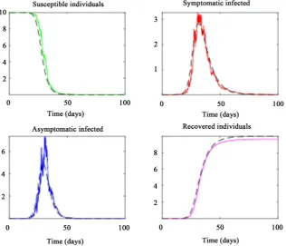
From the description of the dynamics of cholera as shown in Figure 1, we the following set of ordinary differential equation system as in [7].

( )

( ) ( )

( )

( ) ( )

( )

(

) ( )

( )

( ) ( )

( )

(

) ( )

( )

_{( )}

( )

_{( )}

_{( ) (}

_{) ( )}

1

2

1 2

d

, d

d

, d

d

, d

d

, d

d

, d

e s

s a

a

s a

S t B t S t

bN S t

t B t

I t p B t S t

r d I t

t B t

I t q B t S t

r I t

t B t

R t

r I t r I t R t

t B t

I t I t B t

t

β

µ κ

β

µ κ

β

µ κ

µ

α α δ φ

= − −

+

= − + +

+

= − +

+

= + −

= + − +

(1)

with suitable initial conditions. The total human population is given by

( )

e s a

N =S t +I t +I t +R t .

From the model: S t

( )

, I ts

( )

, I ta

( )

, R t

( )

and B t

( )

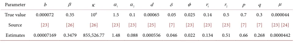
refer to

suscepti-ble individuals, symptomatic infected individuals, asymptomatic infected indi-viduals, recovered individuals and the pathogen concentration in the contami-nated environment respectively. The model parameters are described as follows. b is the birth rate or recruitment rate, β_{is rate of exposure to contaminated}

[image:4.595.210.538.450.692.2]

water,

κ

is the concentration of Vibrio cholerae in water, α1 is the contribution

(5)

of I ts

( )

to the population of Vibrio cholerae through excretion, α2 is the

contribution of I ta

( )

to the population of Vibrio cholerae through excretion,

d death rate due to cholera,

δ

death rate of Vibrio cholerae due to water treatment, φ_{is the mortality rate for bacteria including phage degradation,} r₁ is the recovery rate of symptomatic infected individuals, r2 is the recovery rate

of asymptomatic infected individuals, p is the prob. of new infected from S t

( )

to be symptomatic, q is the prob. of new infected S t

( )

to be asymptomatic ,

µ is the natural death rate.

The key parameter in epidemiology is the basic reproduction number, which is defined as the average number of secondary infectious cases transmitted by a single primary infectious cases introduced into a whole susceptible population

[12]. This parameter is useful because it helps determine whether an infectious disease will spread within the population or not. To compute R0, the next

gen-eration matrix approach is used as in [13]. It is obtained by taking the largest (dominant) eigenvalue value (spectral radius) of

( )

1

0 0 _,

i i

E E −

∂  ∂   _∂   _∂ 

   

 

 

where i is the rate of appearance of new infection in compartment i, i is

the net transition between compartments, E0 is the disease free equilibrium

and i stand for the terms in which the infection is in progression i.e., I ta

( )

,

( )

a

I t and B t

( )

in the model (1). Hence, the basic reproduction number ob-tained in [7] was as follows:

1 2 1 1 2 2 2

0 e,

n

bN

p qr pr dq q

R

D

α βµ α β α β α β α βµ

µ

 + + + + 

=  

  (2)

where

2

1 2 2 1 2

2

1 2 2 1 2.

n

D d r dr r r r

r dr r r r

δκµ δκµ δκµ δκ δκµ δκ δκµφ

φκµ κµφ κφ κµφ κφ

= + + + + + +

+ + + + +

From Equation (2), when R0<1, the highly infectious vibrios will not grow

within human host and the environmental vibrios ingested into human body will not cause cholera infection. But when R0>1 the human vibrios will grow

and persist, and hence leads to human cholera.

3. Stochastic Differential Equations

In this section we provide two approaches of formulating stochastic differential equations from the deterministic model (1). These approaches are parametric perturbation Itô SDEs and Itô SDEs from the transition probabilities.

3.1. Parametric Perturbation Itô SDEs

(6)

( )

1d 1 t

β _β σ+  and dd+σ2d2

( )

t , where 1 and 2 are two

in-dependent standard Brownian motions with the following properties: 1) 0 =0  a.s,

2) For all times 0≤ <s t, the increment  t− s is normally distributed

with zero mean and variance t s− ; i.e.,  t − sN

(

0,t s−

)

,

3) For all times 0< < <t t1 2 <tn, the increments  t1, t2, , tn −tn−1 of

the process are independent random variables,

4) All samples paths 

( )

.,ω : 0,

[

∞ →

)

_,ω∈ Ω, are continuous  a.s. Similarly, σ1 and σ2 are real constants, known as the intensities of the

stochastic environment.

From the deterministic model (1) we get the following system of stochastic differential equations:

( )

( ) ( )

_{( )}

( )

1

( ) ( )

_{( )}

d 1

( )

dS t bN_e B t S t S t dt B t S t t ,

B t B t

β σ

µ

κ κ

 

= − −  −

+ +

 

 



( )

( ) ( )

_{( )}

(

) ( )

( ) ( )

_{( )}

( )

1 1

1

2 2

d

d d

d ,

s s

s

p B t S t pB t S t t

I t r d I t t

B t B t

I t t

β σ

µ

κ κ

σ

 

=_ − + + _ −

+ +

 

 

−



( )

( ) ( )

_{( )}

(

) ( )

1

( ) ( )

_{( )}

1

( )

2

d

dI t_a q B t S t r I t_a dt qB t S t t ,

B t B t

β σ

µ

κ κ

 

=_ − + _ −

+ +

 

 



(3)

( )

1

( )

2

( )

dR t =r I ts +r I ta −µR t d ,t

( )

1

( )

2

( ) (

) ( )

dB t =αI ts +α I ta − δ φ+ B t d ,t

with suitable initial conditions. The technique of parameter perturbation intro-duces another parameters σ1 and σ2 in a model.

3.2. Itô SDEs with Transition Probabilities

This method was proposed by [16][17], the stochastic differential equations fol-low from the diffusion process. The nature of stochastic differential equation to be formulated is in this form:

( )

(

( )

)

(

( )

)

( )

dx t = f t x t, ; dθ t G t x t+ , ; dθ  t , (4)

where G t x t

(

,

( )

;θ

)

is a matrix satisfying _GGT _{= Σ} _[16] _[17]_, _Σ _{is the}

co-variance to order ∆t, Σ∆t is the approximate covariance matrix, 

( )

t is the vector of independent Wiener process, θ is a vector of parameters and

( )

(

, ;

)

f t x t θ is the drift part or deterministic part. From Equation (1) we formulate an equivalent SDEs as

( )

dx t =F t G_td + _td t , (5)

where t

[ ]

x F

t ∆ =

∆

 _and

( )

T

t

x x G

t

_{∆ ∆} 

 

=

∆ 

(7)

such that

( )

[

]

T

1, , ,2 3 4

x t = x x x x . Then, x x x x1, , ,2 3 4, corresponds to the number

of individuals S t I t I t R t

( ) ( ) ( ) ( )

, _s , _a , ∈

[

0,N_e

]

_{respectively and}B t

( )

the Vi-brio cholerae concentration in the environment. However, B t

( )

is not a com-partment occupancy as the other one are so its transition is not considered in the formulation of transitions.

In order to find the expectation 

[ ]

∆x and covariance matrix Σ_{, we need}

to consider the transition probabilities as stated in Table 1. The transition probabilities are formulated from Equation (1). From Table 1, the expectation and variance co-variance matrix are computed as follows:

[ ]

10

( )

1 1 2 2 3 3 4 4 5 5 6 6

1

7 7 8 8 9 9 10 10.

i i

i

E x P x P x P x P x P x P x P x

P x P x P x P x

=

∆ = ∆ = ∆ + ∆ + ∆ + ∆ + ∆ + ∆

+ ∆ + ∆ + ∆ + ∆

∑

₍₆₎

On substituting the values of Pi, ∆xi and

[

]

T

( ) ( ) ( ) ( )

T

1, , ,2 3 4 , s , a ,

x x x x = _S t I t I t R t _ to Equation (6), we get

[ ]

( ) ( )

( )

( ) ( )

( )

(

) ( )

( ) ( )

( )

(

) ( )

( )

1

2

1 2

d

e

s

a

s a

B t S t

bN S t

B t p B t S t

r d I t B t

E x t

q B t S t

r I t B t

r I t r I t R t

β

µ κ

β

µ κ

β

µ κ

µ

 

− −

 ₊ 

 

 ₋ _{+ +} 

 + 

∆ =

 

− +

 ₊ 

 

 ₊ ₋ 

 

[image:7.595.200.538.466.736.2]

and the co-variance matrix is given by

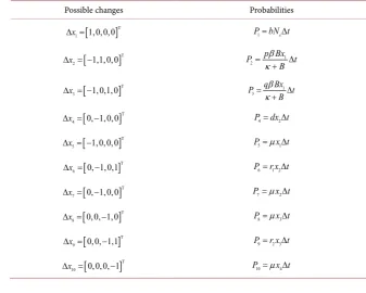
Table 1. Possible changes in the process for the SI I R Bs a − model.

Possible changes Probabilities

[

]

T

1 1,0,0,0

x

∆ = P bN t1= e∆

[

]

T

2 1,1,0,0

x

∆ = − 1

2

p Bx

P t

B

β κ = ∆

+

[

]

T

3 1,0,1,0

x

∆ = − 1

3

q Bx

P t

B

β κ = ∆

+

[

]

T

4 0, 1,0,0

x

∆ = − P dx t4= 2∆

[

]

T

5 1,0,0,0

x

∆ = − P5=µx t1∆

[

]

T

6 0, 1,0,1

x

∆ = − P r x t6= 1 2∆

[

]

T

7 0, 1,0,0

x

∆ = − P7=µx t2∆

[

]

T

8 0,0, 1,0

x

∆ = − P8=µx t3∆

[

]

T

9 0,0, 1,1

x

∆ = − P r x t9= 2 3∆

[

]

T

10 0,0,0, 1

x

(8)

( )

( )( )

(

)(

)

( )( )

(

)(

)

( )( )

(

)(

)

( )( )

(

)(

)

10 _T T 1 T T T

1 1 1 2 2 2 3 3 3

T T

T

4 4 4 5 5 5 6 6 6

T T T

7 7 7 8 8 8 9 9 9

T

10 10 10 .

i i i

i

E x x P x x

P x x P x x P x x

P x x P x x P x x

P x x

= _{∆ ∆} ₌ _∆ _∆   = ∆ ∆ + ∆ ∆ + ∆ ∆ + ∆ ∆ + ∆ ∆ + ∆ ∆ + ∆ ∆ + ∆ ∆ + ∆ ∆ + ∆ ∆

∑

(7)

Also, by substituting the values of Pi, ∆xi and

[

]

T

( ) ( ) ( ) ( )

T

1, , ,2 3 4 , s , a ,

x x x x = _S t I t I t R t _ to Equation (7), we get

( )

( ) ( )

( )

( ) ( )

( )

( ) ( )

( )

( ) ( )

( )

T 2 1 2 2 1 2 3 2 2

1 2 4

0 0 , 0 0 s a s a

E x x

p B t S t q B t S t

B t B t

p B t S t

r I t

B t _t

q B t S t

r I t B t

r I t r I t

β β σ κ κ β σ κ β σ κ σ _{∆ ∆}      − −  ₊ ₊      ₋ ₋   ₊  =_ _∆   − −  +     − −     where

( ) ( )

( )

2

1 e ,

B t S t

bN S t

B t β σ µ κ = + + +

( ) ( )

( )

(

) ( )

2

2 1 s ,

p B t S t

r d I t B t β σ µ κ = + + + +

( ) ( )

( )

(

) ( )

2

3 2 a ,

q B t S t

r I t B t β σ µ κ = + + +

( )

2

4 r I t1 s r I t2 a R t .

σ = + +µ

The Itô stochastic differential equation, where global Lipschitz conditions are satisfied to ensure the existence and uniqueness of strong solution, can be writ-ten as in Equation (4) as found in [14]. Hence by Equation (5), the Itô stochastic differential equations become:

( )

( ) ( )

( )

( ) ( )

( )

(

) ( )

( ) ( )

( )

(

) ( )

( )

1 2 1 2 d d e s a s a

B t S t

bN S t

B t p B t S t

r d I t B t

x t t

q B t S t

r I t B t

r I t r I t R t

(9)

( ) ( )

( )

( ) ( )

( )

( ) ( )

( )

( ) ( )

( )

2

1

2

2 1

2

3 2

2

1 2 4

0 0

d .

0 0

s

a

s a

p B t S t q B t S t

B t B t

p B t S t

r I t

B t _t

q B t S t

r I t B t

r I t r I t

β β

σ

κ κ

β

σ κ

β

σ κ

σ

 

− −

 ₊ ₊ 

 

− − 

+

 

+

 

₋ ₋ 

 ₊ 

 

 ₋ ₋ 

 

 (8)

Note that if I t_s

( )

=I t_a

( )

=0_and B t

( )

=0_{, then cholera epidemic stops.}

4. Analysis of Parametric Perturbation Itô Stochastic

Differential Equation Model

In this paper, unless otherwise stated, we let

(

Ω, , 

{ }

t ,

)

be a complete

fil-tered probability space, with

{ }

_{t t}≥₀ satisfying the usual conditions (i.e.,

in-creasing and right continuous also 0 contains all -null sets). Let

4

1 2 3 4

: bNe ,

x x x x x

µ

+

 

∆ =_ ∈ + + + < _

  

where

( )

1 , 2 s , 3 a , 4 .

x =S t x =I t x =I t x =R t

4.1. Global Existence and Uniqueness of Positive Solutions

Before proving the existence and uniqueness of positive solutions, let us state the conditions that guarantee the existence and uniqueness of solution of Equation (4).

Lemma 1. Assume that there exist two positive constants _Kˆ_{and K such that}

1) (Lipschitz condition) for all _{x y}, _∈_n_and

[

]

0, t∈ t T

( )

_,

( )

_, 2 _ˆ 2

f x t − f y t ≤K x y−

2) (Linear growth condition) for all

( )

[ ]

( )

2

(

2

)

0

, n , , 1 .

x t ∈_ × t T f x t ≤K + x

Theorem 1. For any initial value

(

( ) ( ) ( ) ( ) ( )

_{0 ,} _{0 ,} _{0 ,} _{0 ,} ₀

)

5

s a

S I I R B ∈+ ,

there is a unique solution x t

( )

=S t I t I t R t B t

( ) ( ) ( ) ( ) ( )

, _s , _a , , _{to system}₍₃₎_for

all t≥0_{, and the solution will remain in} 5 +

 with the probability 1, namely

( )

5

x t ∈+, for all t≥0 almost surely.

Proof. Since the coefficients of system (3) satisfy the local Lipschitz condition, then for initial values

(

( ) ( ) ( ) ( ) ( )

_{0 ,} _{0 ,} _{0 ,} _{0 ,} ₀

)

5

s a

S I I R B ∈+, there is unique

lo-cal solution S t I t I t R t B t

( ) ( ) ( ) ( ) ( )

, s , a , , on

[

0,νε

]

, where νε is the first hit-ting time or explosion time. In order to prove that the solution is global and pos-itive, we need to show that ν = ∞_ a.s. Let k0>0 be sufficiently large so

that S

( ) ( ) ( ) ( ) ( )

0 ,Is 0 ,Ia 0 , 0 , 0R B remain within the interval 0 0

1 ,k k

 

 

(10)

integer k k≥ 0. Let νk:Ω

[ ]

0,∞ be any random variable (taking eventually

infinite value) on a filtered probability space

(

Ω, , 

{ }

t ,

)

. We say that νk is

a stopping time for filtration t if at each (deterministic) time t≥0, the event

[

νk ≤t

]

is known in t. In this study we define

[

) ( )

1

inf 0, : , for some ,1 5

k t k x ti _k k i i

ν

= _ ∈

ν

∉_ _ ≤ ≤ _

 

 

Let ∅_{be empty set then the}inf∅ = ∞. By definition νk increases as

k→ ∞_{. Let}ν∞ =limk→∞νk, then ν∞≤νε a.s. We need to show that ν∞ = ∞ a.s. Then ν = ∞ε and x t

( )

∈5+. If this statement is false we say that, there

exist ε∈

( )

0,1 _{and a constant}T >0_{, such that}

{

ν_∞ ≤T

}

>ε. As a conse-quence to this, there exist an integer k1 >k0 such that

{

νk ≤T

}

≥ε, ∀ ≥k k1

 (9)

For t≤νk and at each k,

(

)

(

)

(

)

d d

d ,

s a s a s

s a

S I I R S I I R dI t

S I I R t

µ µ

 

+ + + = Λ −_ + + + − _

 

≤ Λ −_ + + + _ (10)

where Λ =bNe. Then

( )

0

0 0

if

: , if

s a

N

S t I t I t R t

N N

µ µ

µ

Λ Λ

 _≤



+ + + ≤ _Λ =

 _≥



 (11)

where

( )

0 0 s 0 a 0 0 ,

N =S +I +I +R

and

0

max ,N .

µ

Λ 

= _ _

 



Define now _1,2_{the Lyapunov function}_V_: 5 +→ +

  by

(

)

(

)

(

) (

)

(

) (

)

, , , , 1 In 1 In 1 In

1 In 1 In ,

s a s s a a

V S I I R B S S I I I I

R R B B

= − − + − − + − −

+ − − + − − (12)

and S t I t I t R t B t

( ) ( ) ( ) ( ) ( )

, _s , _a , , ∈ Ω_{. Then}V x t t

(

_{( )}

,

)

is an Itô stochastic process with the SDEs given by

( )

(

)

( )

(

)

(

( )

)

( )

(

( )

(

( )

)

( )

)

( )

(

)

( )

T

d ,

1

, , trace , d

2

, d ,

t x xx

x

V x t t

V x t t V x t t f t g t V x t t g t t

V x t t g t t

 

=_ + + _

 

+ 

(13)

which becomes

( )

(

)

(

( )

)

( )

dV x t t, =LV t V x t t g td + x , d t , (14)

(11)

(

)

(

)

(

)

(

)

(

)

1

2 1 2

2 2 2 1

1 2 2 2

2 2 2 2 2 2

2 2

1 1

2

2 2 2

1 1 1 1 1 1 1 1 1 1 1 d 2

1 _d 1

2 2

s s

a s a

a

s a

s

s a

BS p BS

LV S r d I

S B I B

q BS _{r I} _{r I} _{r I} _R

I B R

B S

I I B t

B S B

p B S _I _t q B

I _B I

β _µ β _µ

κ κ

β _µ _µ

κ

σ

α α δ φ

κ

σ _σ σ

κ

 

= −_ _Λ − − + −_ _ − + +

+ +   _ _     + −_ _ − + + −_ _ + − +         + −_ _ + − + +     _ + _   +  +  + +    

(

)

2 2 2 d S _t B κ     +     Hence

(

)

(

)

(

)

1 2 1

2 2 2 2 2 2

1 1

2 1 2 2 2 2

2 2 2 2 2

2 1 2 2 2 2 , 2 2 s

a s a

s

a

B p BS q BS

LV r d r r I

B B B

B p B S

r I I I

B I B

q B S

I B

β _µ β _µ β _µ

κ κ κ

σ σ

µ α α δ φ

κ κ

σ σ

κ

≤ Λ + + + + + + + + + +

+ + + + + + + + + + + + + + + + (15)

From max

_µ

,N0

Λ 

= _ _

 

 , it follows that

(

)

₍

₎

₍

₎

1 2 1 2

2 2 2 2 2 2 2 2 2 2 2

1 1 2 1

2 1

2 2 2

2 4

2 2 2 2

: ,

a s

p B q B B

LV r r

B B B

B p B _{r r d} q B

B I B I B

β β _{α α} β _{δ φ}

κ κ κ

σ σ σ _µ σ

κ _κ _κ

 

≤ Λ +_ + + + + + _ + + +

+ + +   + + + + + + + + + + + =     (16)

where  is a positive constant independent of variables S I I R B, , , ,s a and

time t. Then we obtain

( )

_{( )}

1 1 1 1

2 2

d d

1

d d d ,

s a

pB t qB t

S S

V t t

I p B I B

σ σ σ κ κ   ≤ −_ − _ − − + +  

    (17)

let ν_k∧ =T min

{

ν_k,T

}

_{. Introduce integral to Equation (17)}

( ) ( ) ( ) ( ) ( )

(

)

( )

0 1 1 0 0 1 1 2 2 0 0

d , , , ,

d 1 d d d . k k k n n T s a T T s T T a

V S s I s I s R s B s

pB s

S s

I p B

qB s S s I B ν ν ν ν ν σ κ σ σ κ ∧ ∧ ∧ ∧ ∧   = − _ − _ +   − − +

∫

    (18)

Introducing the expectation to Equation (18) and by the Gronwall inequality, leads to

(

) (

)

(

_k , _s _k , _a _k , _k , _k

)

,

V S ν T I ν T I ν T Rν T Bν T C T

 ∧ ∧ ∧ ∧ ∧ ≤ +

 

  (19)

where C V S=

(

( ) ( ) ( ) ( ) ( )

0 ,I_s 0 ,I_a 0 ,R 0 ,B 0

)

_{. Since the mean of stochastic}

integral equals zero [18]. Then let Ω =k

{

νk ≤T

}

,∀ ≥k k1 from inequality (9),

(12)

(

_k, ,

) (

_s _k, ,

) (

_a _k, ,

) (

_k, ,

) (

_k, ,

)

S ν T I ν T I ν T R ν T Bν T

which can take either 1_k or k. Hence we have

(

) (

)

(

)

( )

, , , , , , , , ,

1 1

1 log 1 log ,

k s k a k k k

V S T I T I T R T B T

k k

ν ν ν ν ν

  

≥_ − − _∧_ − − _{ }_  

 

(20)

again define the indicator function on Ωk denoted by  be defined for all k

ω ∈ Ω _by

( )

1 if_{0 otherwise}

k

ω

Ω

∈ Ω 

=   



From Equation (19) and by Bienayme Chebyshev inequality we have

(

) (

)

( )

, , , , , , , , ,

1 1

1 log 1 log ,

k k s k a k k k

C T S T I T I T R T B T

k k

ν ν ν ν ν

Ω

 

+ _{≥ } _

  

≥ _ − − ∧ − − _{ }_

 

  

 (21)

when k→ +∞, this leads to contradiction as

( ) ( ) ( ) ( ) ( )

(

0 , _s 0 , _a 0 , 0 , 0

)

V S I I R B T

∞ > +_ = ∞

Therefore, we conclude that for the solution S t I t I t R t B t

( ) ( ) ( ) ( ) ( )

, _s , _a , , of cholera model not to explode at finite time with probability 1, we need to have ν_∞ = ∞_{a.s. This completes the proof.}□

Theorem 1 shows that the solution of model (3) will remain in 5 +

 . Next, we give the definition of stochastic ultimate boundedness [19], which is very im-portant in population dynamics.

Definition 1. The solution x t

( )

=

(

S t I t I t R t B t

( ) ( ) ( ) ( ) ( )

, _s , _a , ,

)

_{of model}₍₃₎

are said to be stochastically ultimately bounded, if for any ∈

( )

0,1 , there is a positive constant δ δ=

( )

 , such that for any initial value

( ) ( ) ( ) ( ) ( )

(

)

5

0 0 , s 0 , a 0 , 0 , 0

x = S I I R B ∈+, the solution x t

( )

to Equation (3)

has a property that

( )

{

}

limsup .

t→∞  x t >δ <

Theorem 2. The solutions of system (3) are stochastically ultimately bounded for any initial value 5

0 x ∈+.

Proof. From Theorem 1, we showed that S t I t I t R t B t

( ) ( ) ( ) ( ) ( )

, _s , _a , , re-main in 5

+

 , for all t≥0_{almost surely.}

Let V1, V2 and V3 be lyapunov functions stated as

1 et , 2 e ,t s 3 et a where 1.

V ₌ Sθ V ₌ Iθ V ₌ Iθ _θ_> ₍₂₂₎

Taking their derivatives with respect to θ we get

( )

1 2 3

e e

et _, t _and t _.

s a

I I

S

V V V

S I I

θ θ

θ

_θ

θ

′ = ′ = ′ = ₍₂₃₎

Using Itô formula we get

( )

1 1

e d dV LV td B St t ,

B

θ σ θ

κ

= −

+

(13)

( )

_{( )}

1 1

2 2 2 2

e d

d d t e dt ,

s

p B S t

V LV t I t

B

θ

σ θ _{σ θ}

κ

= − −

+



 (24)

( )

1 1

3 3

e d

dV LV td q B St t ,

B θ σ θ κ = − +  but

( )

(

T

( )

)

1

1 1 1 trace₂ 1 1 1 ,

V

LV V f t g t V g t

t θ θθ

∂

= + +

∂

( )

(

T

( )

)

2

2 V 2 1 trace₂ 2 2 2 ,

t θ θθ

∂

= + +

∂ (25)

( )

(

T

( )

)

3

3 V 3 1 trace₂ 3 3 3 ,

t θ θθ

∂

= + +

∂

where

(

)

(

)

(

)

1 2 2 2 3 2

1 e 1 e 1 e

, , ,

t t t

s a

S I I

V V V

S I I

θ θ θ

θθ θθ θθ

θ θ− θ θ− θ θ−

= = = ₍₂₆₎

( )

1

( )

1

( )

1

1 , 2 2 s , 3 .

BS pBS qBS

g t g t I g t

B B B

σ

_σ

σ

κ

−

     

=_ _ =_ − _ =_ _

+ + +

      (27)

Therefore

(

)

(

)

2 2 1 1 2 1 e 1

e 1 ,

2

t

t B S B

LV S

S B B

θ

θ _θ β _µ θ θ σ

κ κ

−

 Λ 

= _ + _ − − __+ +   +  

(

)

₍

(

₎

)

(

)

2 2 2 2 1

2 1 2 2

2 2 1 e 1 e 1 2

1 _{1 e ,}

2 t s t s s s t s

p B S I

p BS

LV I r d

I B I B

I

θ θ

θ

σ θ θ

β

θ µ

κ _κ

σ θ θ

   − =  + _ − − − _+ + +      + − (28)

(

)

(

)

2 2 2 2 1

3 2 2 2

1 e 1

e 1 .

2 t a t a a a

q B S I

q BS

LV I r

I B I B

θ

θ _θ β _µ σ θ θ

κ κ    − =  + _ − − _+ + ₊     

There exists positive constants 1, 2 and 3 such that

1 1e ,t 2 2et and 3 3e .t

LV < LV < LV < (29)

It follows that

( )

(

)

(

( )

)

(

( )

)

(

( )

)

( )

(

)

(

( )

)

1 2 3

0 , 0

and 0 .

s s

a a

S t S I t I

I t I

θ θ θ θ

θ θ

− ≤ − ≤

− ≤

     

   (30)

Then

( )

1 2

3

limsup , limsup

and limsup .

s

t t

a t

S t I t

I t

θ θ

θ

→∞ →∞

→∞

 ≤ < ∞  ≤ < ∞

   

  ≤ < ∞

 

   

  (31)

For

( )

(

( ) ( ) ( )

_, _,

)

3

s a

x t = S t I t I t ∈+ and consider the case of 0< <θ 3.

(14)

( )

(

( )

)

{

( ) ( ) ( )

}

( )

{

}

2 2 2 2 2

2

3 max , ,

3

s a s a

s a

x t S t I t I t S t I t I t

S t I t I t

θ θ

θ _θ _θ _θ

θ

θ θ θ

= + + ≤

≤ + +

(32)

consequently we have

( )

2

4

limsup 3 ,

t x t

θ

→∞  ≤  (33)

where 4 >0 is a suitable constant.

There exists a positive constants δ1 such that

( )

1

limsup .

t→∞  x t ≤

δ

Given >0 and let 12

2

δ

δ =

 , then by Bienayme Chebyshev inequality

( )

{

x t

δ

}

x t

( )

.

δ

> ≤

 (34)

Hence

( )

{

}

1

limsup .

t x t

δ δ

δ

→∞  > ≤ =

This completes the proof as required. □

4.2. Moment Exponential Stability

The moment exponential stability of the equilibrium solutions of stochastic differential Equation (3) are established from the idea of Lyapunov function

[20].

Lemma 2. Consider a function 1,2

(

n

[ ]

_t_{, ;}

)

+

× ∞

   satisfying these inequa-lities:

( )

1 , 2

p p

M x ≤V x t ≤M x

and

( )

, 3

p

LV x t ≤ −M x , _t_{≥ ∀}0,

( )

_{x t}, _∈_n_{× ∞}

[ ]

_t,

where M M M1, 2, 3 and p are positive constants. Then the equilibrium solution

of Equation (3) is pth moment exponentially stable. When p=2, it is usually said to be exponentially stable in mean square and the DFE is globally asymptot-ically stable.

Lemma 3. When p≥2_and x y, ,>0. Then

(

)

(

)

(2 )2

1 1 p 1 1 _and 2 2 2 p 2 _e p _.

p p x p p p p x p

x y y x y y

p p p p

− − _≤ −  ₊ _− − _≤ −  ₊

Theorem 3. If R0<1 and p≥2, the disease free equilibrium of the model

system (3) is pth moment exponentially stable in ∆_.

Proof. Given that

(

S

( ) ( ) ( ) ( ) ( )

0 ,Is 0 ,Ia 0 ,R 0 ,B 0

)

∈ ∆, as from Theorem 1

the solution of the system remains in ∆_{. Set} p≥2_{, then consider Lyapunov}

function 1 3 4 5

p _p

p p p

s a I

V S I R B

p

λ λ λ λ

µ

Λ 

= _ − _ + + + +

(15)

(

)

(

)

(

)

(

)

(

)

(

)

1 1 1

1

1 1

2 _{2 2 2} 1 1

1 2 1

2 2 2 2

2 1 2 2 1

3 2 2 4 1 ₁ 2 1 ₁ 2

p p p

p

p s

s s

p s p

s s a a

p

p BS

LV p S S p S S

B

p BS B S

p p S I r d I

B B

p B S q BS

p I I pI r I

B B

pR

λ β

λ λ µ

µ κ µ µ

β σ

λ µ

µ _κ κ

σ _σ _λ β _µ

κ κ λ − − − − − − − −

Λ  Λ  Λ 

= − Λ_ − _ + _ − _ + _ − _

+

     

Λ   

+ − _ − _ + _ − + + _ +   +     _ _   + − + + _ − + _  +   +    +

(

)

(

)

(

)

(

)

1 1

1 2 5 1 2

2 2 2 2 2 1

3 2

1 ₁ _.

2

p

s a s a

p a

r I r I R pB I I B B

q B S

p p I

B

µ λ α α δ φ

σ λ κ − − + − + + − − + − + (35)

In ∆ _{, we have}S

( ) ( ) ( ) ( ) ( )

0 ,Is 0 ,Ia 0 , 0 , 0R B

_µ

,0,0,0,0

Λ 

∈ 

 , such that

S≤_µΛ, then from the fact that B 1

B

κ+ ≤ , as B∈

[ ]

0,1 , there exists η∈

[ ]

0,1

such that 2

(

2 2

)

2 1 2

2

n

x y S x y

η

µ

−

Λ ₊ _≤

, Then LV becomes

(

)

(

)

(

)

(

)

(

)

(

)

1 1 1 1 2 2 2 1

1 1 2 1

2

2 2 2 2 1

1 2 2 3

1 1 1

3 2 4 1 4 2 4 5 1

5 2

1 ₁

2

1 ₁ 1 ₁

2 2

p p

p

p p

s s s

p p p

s s s a

p p p p p

a s a s

LV p S p S

p p S p I r d I

p p I p I qp I

p r I pr I R pr I R pR pI B

λ β µ λ

µ µ µ

λ ησ β µ

µ µ

µ

η σ σ λ β

µ µ

λ µ λ λ λ µ λ α

λ α − − − − − − − − −

Λ  Λ Λ 

≤ − Λ_ − _ + + _ − _

   

 

Λ Λ Λ

+ − _ − _ + − + +

 

Λ Λ

+ − + − +

− + + + − +

+ 1

(

)

(

)

2 2 2 2

5 3 1 2

1 ₁ _.

2

p p p

a a

pI B λ p δ φ B λ p p ησ q I

µ

− ₋ ₊ ₊ ₋ Λ −

(36)

Applying the idea of Lemma 3, we can formulate some of the inequalities as follows

1 1 1 1 _,

p p p p

s p s

I R R I

p p

− _≤ − _ ₊ _−

2 2

2 2 2 2 _,

p p p

p

s p s

I S S I

p p

µ µ

− −

Λ₋  _≤ − Λ₋  ₊

   

     (37)

1

1 1 _.

p p

e p e

N S S N

p p

µ µ

−

Λ₋  _≤ − Λ₋  ₊

   

    

On substituting these inequalities in Equation (19), we get

(

)

(

)

(

)

(

)(

)

(

)(

)

(

)

(

)

(

)

(

)

(

)

(

)

1 1 2 2 2 2 2

1 1 2 1

2

1 2 4 1 4 2

5 2 5 1

1 1

1 ₁ ₂ ₁ ₂

2 2

1 ₁ ₁ ₁

2

1 1 1

p p

p P

s

p p p

s

p p s p

s b

LV b p S p S

p

b b

p p S p p S

p

r d p I p r R p r R

p

p B p B p I

p

λ β µ λ

µ µ µ

λ ησ ησ

µ µ µ

µ

µ σ λ λ

λ α λ α β

µ

Λ  Λ 

≤ − − _ − _ + + − _ − _

   

Λ  Λ 

(16)

(

)

(

)

(

)

(

)(

)

(

)(

)

3 3 2 4

2 2 2

5 3 1 2

2

2 2 1 1

1 2 4 1 4 2

1 1

5 1 5 2

1

1 ₁ ₂

2

1 ₁ ₂

2

.

p p p

a a

p p

p p p p p

s s s a

p p p p

s a

q p I p r I pR

b

p B p p q S

b

p p p I r I r I

p

I I

λ β λ µ λ µ

µ

λ δ φ λ ησ η

µ µ

η σ λ λ

µ

λ α λ α

− −

Λ

+ − − + −

Λ 

− + + − − _ − _   + − − + + + +       (38) Hence

(

)

(

)

(

)(

)

(

)

(

)

(

)

(

)

(

)

(

)

(

)

2 1 2

2 2 1 1

1 2 4 1 5 1

1 2 4

1 2 5

1 1

2 3 4 2 5 2

1 ₁ ₁

2

1 ₁ ₂

2 1 1 1 1 1 s s

p p p

s s

p

p p p

a

p

LV r d p p

p

b

p p p r I

p

r p r p p R

p p p B

q

p b p r r I

µ σ β

µ

η σ λ λ α

µ

µ λ

δ φ α α λ

β µ λ λ λ α

µ − − − −  Λ ≤ −_ + + − − + −   − − − − − _  −_ − + − + _ −_ + + − + − _    −__ − + + _ − − _              

(

)

(

)

(

)

(

)

(

)

2 2

1 2 1 1

2 2

1 1 2 2

1 1 1 2 1

2 2

1 2 2 2

1 2 2

1 ₂ ₁

2 1 1 _, p p p p p p p s s e b b

b p F p S

b b

b p

p b p _p b _{F N}

p p

µ β ησ λ

µ µ µ

λ β µ λ ησ η λ

µ µ

β η σ

µ µ

−

− −

  Λ 

− −_ + − − − _ − _ − _      −_ − + − −   − − − −        (39)

where 2

(

)

2 2 3

(

)

12 2 2

1 2 1 2

1 1 2 2 2 2 s p q p b

F p b

p

λ ησ

ησ

λ

µ λ µ

−

= − + _and

(

)

2 2

1 2 2 2

2 3 3 1 1 2

p p

b b

F λ βq λ p ησ q

µ µ

− −

=  + −  . If we choose  sufficiently very

small, then we can choose λ λ λ λ λ1, , , ,2 3 4 5 positive such that the coefficients

, , , , ,

p

p p p p p

s a e

S I I R B N

µ

Λ₋ 

 

  become negative.

Hence, according to Lemma 2 the proof is complete. □

4.3. Almost Sure Convergence

Theorem 4 If R0<1, then I t I t R ts

( ) ( ) ( )

, a , converge almost surely

expo-nentially to (0, 0, 0).

Proof. Let

(

S

( ) ( ) ( ) ( )

0 ,Is 0 ,Ia 0 ,R 0

)

∈ ∆. As R0<1, define the lyapunov

function as V I I R

(

s, ,a

)

=In

(

I ts

( )

+I ta

( )

+wR t

( )

)

, such that w>0. Using Itô

(17)

( )

(

)

(

)

(

)

( )

(

)

(

)

(

)

( )

( )(

)

( )

(

) ( )

( )

1

2 1 2

2 2 2 2 2 2 2 2

2 2

1 1

2

2 2 2

1 1 2 2

1 1 1 d d 1 _d 2 d d d . s s a

a s a

s

s a

s

s a s a

s a

p BS

V r d I

I t I t wR t B

q BS _{r I} _{w r I} _{r I} _R _t

B

p B S _I q B S _t

B B

I t I t wR t

pBS t I t

I t I t wR t B I t I t wR t

qBS t

B I t I t wR t

β _µ

κ

β _µ _µ

κ

σ _σ σ

κ κ σ σ κ σ κ  = _ − + + + +  +  + − + + + − _ +      − + +  ₊ ₊  + + _ _ + + + + + + + + + + +    (40)

But p q+ =1, also by dropping some of the negative terms in Equation (40) we obtain

( )

(

)

(

)

(

)

₍

_{) ( )}

_{( )}

( )

(

) ( )

( )

1 2 1 1 1 2 1 1 2 2 1 d d d d d _. s a s a s a s a s

s a s a

BS

V r d I r I

pBS

w r I r I R t

qBS t

I

I t I t wR t B I t I t wR t

β _µ _µ

κ σ µ κ σ σ κ  ≤ _ − + + − + + +  +  + + − _ + + + +  + + + + + + +    (41)

( )

(

)

( )

( ) (

)

(

) ( )

( )

(

) ( )

( )

1 1 2 2 2 2 1 1 1 1 1 d d 1 _d d d d . s s a a s a s

s a s a

s a

BS

V r d wr I t

r wr I w R t

I t I t wR t

I pBS

B I t I t wR t I t I t wR t

qBS t

β _µ κ µ µ σ σ κ σ κ   ≤ _ − + + − _ + +  +  + _− + − − _ + + + + + + + + + + + + +    (42)

When R0<1, then disease die out and hence B=0. Therefore

( )

( ) (

)

( )

( ) (

)

( )

1 1 2 2 2 2 1 d d 1 _d d _. s s a a s a s s a

V r d wr I t

I t I t wR t

r wr I w R t

I t I t wR t

I

I t I t wR t

µ µ µ σ ≤ _− + + − _ + + + _− + − − _ + + + + +  (43)

Let θ =min

(

µ+ + −r d wr1 1,µ+ −r wr w2 2, µ

)

. It follows that

( )

2

( )

d 2

( )

d d s .

s a

I

V t

I t I t wR t

σ

θ

≤ − + + +  (44)