Visual analytics of delays and interaction in movement data

Full Terms & Conditions of access and use can be found at

http://www.tandfonline.com/action/journalInformation?journalCode=tgis20

Download by: [University of St Andrews] Date: 02 February 2017, At: 04:07

International Journal of Geographical Information

Science

ISSN: 1365-8816 (Print) 1362-3087 (Online) Journal homepage: http://www.tandfonline.com/loi/tgis20

Visual analytics of delays and interaction in

movement data

Maximilian Konzack, Thomas McKetterick, Tim Ophelders, Maike Buchin,

Luca Giuggioli, Jed Long, Trisalyn Nelson, Michel A. Westenberg & Kevin

Buchin

To cite this article: Maximilian Konzack, Thomas McKetterick, Tim Ophelders, Maike Buchin, Luca Giuggioli, Jed Long, Trisalyn Nelson, Michel A. Westenberg & Kevin Buchin (2017) Visual analytics of delays and interaction in movement data, International Journal of Geographical Information Science, 31:2, 320-345, DOI: 10.1080/13658816.2016.1199806

To link to this article: http://dx.doi.org/10.1080/13658816.2016.1199806

© 2016 The Author(s). Published by Informa UK Limited, trading as Taylor & Francis Group

Published online: 21 Jun 2016.

Submit your article to this journal

Article views: 339

View related articles

Visual analytics of delays and interaction in movement data

Maximilian Konzacka_{, Thomas McKetterick}b_{, Tim Ophelders}a_{, Maike Buchin}c_,

Luca Giuggiolid_{, Jed Long} e_{, Trisalyn Nelson}f_{, Michel A. Westenberg}a

and Kevin Buchina

a_{Department of Mathematics and Computer Science, TU Eindhoven, Eindhoven, The Netherlands;}b_Bristol

Centre for Complexity Sciences, University of Bristol, Bristol, UK;c_{Fakultät für Mathematik, Ruhr-Universität}

Bochum, Bochum, Germany;d_{Department of Engineering Mathematics, University of Bristol, Bristol, UK;} e_{School of Geography & Geosciences, University of St Andrews, St Andrews, UK;}f_{Department of}

Geography, University of Victoria, Victoria, Canada

ABSTRACT

The analysis of interaction between movement trajectories is of inter-est for various domains when movement of multiple objects is con-cerned. Interaction often includes a delayed response, making it difficult to detect interaction with current methods that compare movement at specific time intervals. We propose analyses and visua-lizations, on a local and global scale, of delayed movement responses, where an action is followed by a reaction over time, on trajectories recorded simultaneously. We developed a novel approach to compute the global delay in subquadratic time using a fast Fourier transform (FFT). Central to our local analysis of delays is the computation of a matching between the trajectories in a so-called delay space. It encodes the similarities between all pairs of points of the trajectories. In the visualization, the edges of the matching are bundled into patches, such that shape and color of a patch help to encode changes in an interaction pattern. To evaluate our approach experimentally, we have implemented it as a prototype visual analytics tool and have applied the tool on three bidimensional data sets. For this we used various measures to compute the delay space, including thedirectional distance, a new similarity measure, which captures more complex interactions by combining directional and spatial characteristics. We compare matchings of various methods computing similarity between trajectories. We also compare various procedures to compute the matching in the delay space, specifically the Fréchet distance, dynamic time warping (DTW), and edit distance (ED). Finally, we demonstrate how to validate the consistency of pairwise matchings by computing matchings between more than two trajectories.

ARTICLE HISTORY Received 17 July 2015 Accepted 2 June 2016

KEYWORDS

Trajectory analysis; visual analytics; similarity measures

1. Introduction

In a wide range of applications, such as biology, urban planning, sports, or ecology, movement data are being collected in the form of trajectories. In recent years, technol-ogy advances have led to a rapid improvement in the ability to record trajectory data

CONTACTMaximilian Konzack [email protected]

Present address of Trisalyn Nelson is School of Geographical Sciences and Urban Planning, Arizona State University, Tempe, Arizona

VOL. 31, NO. 2, 320_–345

http://dx.doi.org/10.1080/13658816.2016.1199806

© 2016 The Author(s). Published by Informa UK Limited, trading as Taylor & Francis Group

(Nathan and Giuggioli 2013). New technology allows scientists to collect data of high resolution, long durations and for a large number of simultaneously moving entities.

Coupled with methodological advancements movement data offer an opportunity to

better understand the mechanisms and behavioral ecology guiding collective motion. In order to explore such data interactively, this research integrates interaction and delayed responses on movement data in a new visual analytics tool.

Interactionis the interdependency in the movements of two trajectories (Doncaster

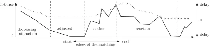
1990). The computation of interaction events is motivated by understanding combined movements of separation, attraction, or mutual repulsion between the moving objects. One way to identify interaction is to compute an alignment between the trajectories. Within an alignment, any point of one moving object is mapped to another point or a range of points from the other moving object. We are interested in exploring delayed responses in the movement, where one moving object moves into a new direction, an action pattern, and this is followed by an adaption of the other moving object, a reaction pattern, over time. To capture such patterns, we need the so-called interaction measures, which are similarity measures adapted to cover aspects of interaction. An example of such anaction–reaction patternis depicted inFigure 1.

Delayis the temporal difference for a pair of points from the trajectories. InFigure 1

the progression of delays is visualized as a dotted curve. Either positive or negative delays can occur over time, depending on whether thefirst point of the pair has a larger time stamp than the second one or vice versa. A positive delay corresponds to thefirst point being delayed, while a negative delay corresponds to the second point being delayed.

Using the direction of movement and the displacement at corresponding time stamps of the trajectories, Long and Nelson (2013) define the dynamic interaction measurefor the calculation of strength and degree of interaction between the moving objects. However, interaction often includes a delayed response. For example, delays are expected in interaction movement patterns for behaviors associated with pursuit and escape, confrontation, and avoidance (Merki and Laube2012).

Computational methods for detecting a delayed response often search for movement episodes from two trajectories with similar characteristics but with a delay for one of the trajectories. Reaction delay is a key parameter in ascertaining leadership and causality,

decreasing interaction

adjusted action reaction

0

0

edges of the matching

start end

distance delay

delay

since a moving entity requires time to perceive, process, and respond to the motion of its neighbor. Hence, the movement patterns are characterized by periods of interactive and noninteractive behavior. Such an episode refers to one period over time, and it might, therefore, be expressed as a sequence of points ranging from one point to all of them. This depends on the level of analysis of the interactive behavior. The scope of the analysis can be varied from a local analysis over episodes to a global analysis. A local analysis reveals the times and locations of dynamic interactions, and it allows a finer treatment of the interaction itself (Long and Nelson2013).

A‘follow-behind’pattern is detected in Buchinet al. (2008) byfinding episodes where two trajectories move through approximately the same locations but with a small delay. Nagyet al. (2010) compute a similar pattern by looking at how a trajectory copies the direction of movement of another with a delay. Using a time-ordering procedure to analyze the cross-correlation of velocity and distance, Giuggioli et al. (2015) extract interaction delays and are able to classify copying patterns in both space and direction.

There is a wide range of alignment methods, e.g., dynamic time warping (DTW)

(Berndt and Clifford1994),edit distance on real sequences (EDR) (Chenet al.2005), and theFréchet distance(Alt and Godau1995), that aim at simply identifying similar move-ment. We discuss these methods in more detail inSection 4.2.

In movement analysis there is a growing interest in analysis methods that include visualizations. Andrienkoet al. (2013) analyze delayed responses in the context of group movement. To identify a group ordering over time, they precomputefirstly a centroid on the collection of trajectories, and rank then the interaction of a trajectory and the centroid for each trajectory of the group. One pattern that they detect is the direc-tion-based delay pattern by Nagyet al. (2010). Its occurrence is visualized in space and time.

Our aim is a visual analytics approach to explore delayed responses in the form of

action–reaction patterns. For this purpose we propose an approach to analyze and

visualize delays in two trajectories. We expect that the trajectories have been recorded simultaneously and with the same sampling rate such that the input data captures spatial and temporal relationships at the same time.

Although our focus is on pairs of trajectories, we also show the application of our methodology to a set of three simultaneous trajectories. Computing and visualizing an

alignment on k trajectories is cumbersome since the computational time of current

state-of-the-art techniques for alignments grows exponential in the number of trajec-tories. Thus, it is inherently demanding to develop an interactive visualization for k

trajectories that captures interaction events.

To determine whether two trajectories have interactions at all, we develop a new approach to compute a global correlation in subquadratic time in the length of the trajectories (seeSection 3). The global measure captures the overall interaction between the moving objects by computing the correlation via the fast Fourier transform (FFT) and approximates the global delay under an interaction measure.

of the matching with respect to certain features of the trajectories. The temporal alignment is then used, which is induced by a matching, to analyze the delay. This approach scales up to hundred points in the trajectories, since it visualizes the trajec-tories and their interaction patterns as a whole. This approach is summarized in

Section 4.

In this article, we conduct new, extensive experiments on the FFT approach and the matching-based approach on three data sets (seeSection 5). We compare these results to those obtained by the time-ordering approach by Giuggioli et al. (2015), DTW, and others. We extend the matching-based approach to three trajectories in order to relate the result on the interaction among the three moving objects with a pair-wise analysis of the triplet.

2. Interaction and similarity measures

Measuring interaction is closely linked to measuring similarity. In this section, we describe properties of these measures and review interaction measures used in our tool. Trajectory data can be represented as a sequence of points over time. Hence, it consists of directions and locations. Interaction measures can be distinguished into these types. We are interested in different facts of interaction. By combining existing measures into a single measure, the combined measure expresses more complex inter-actions. In this work, we analyze only discrete trajectories to have a well-defined delay.

Definition 2.1: A discrete trajectory T is a sequence of n time-stamped points

hðp1;t1Þ;ðp2;t2Þ;. . .ðpn;tnÞi, where each pi2Rd and each ti2Rþ for i2f1;. . .;ng. T

(t) selects the corresponding point in the trajectory for a valid time stampt.

For a pair of points from the trajectories, a delayis a time difference of the

corre-sponding time stamps. Without loss of generality, we assume that a delay τ has a

discrete value between 0 and n – 1. The sampling rate of the underlying data set is

then multiplied withτto obtain an actual delay, e.g., in seconds.

Before elaborating on the interaction measures that we used in our algorithms for computing a matching, we look at common properties that these measures should provide. Without loss of generality, we presume that the measures are given as a distance, i.e., smaller distance values correspond to higher similarity. A distance can be easily transformed into a similarity measure and vice versa.

Definition 2.2:A metric on a set X with d:XX!Rsatisfies the following conditions for allx, y, z∈ X

dðx;yÞ 0 (i)

dðx;yÞ ¼0 iff:x¼y (ii)

dðx;yÞ ¼dðy;xÞ (iii)

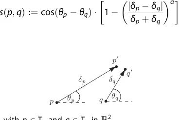
Given a pair of pointsðp;qÞ 2RdRdon trajectories T1and T2, a similarity measure can be computed from spatial properties or the direction of the movement (p, q). The movement vector pp′ is the directed line segment fromp to the consecutive pointp′

with lengthδp. The same holds for qrespectively.

Thedirectionofpin T1measures an angleθpon the movement vectorpp′with regard

to some other criteria. Very frequently, theheadingis used, which is an angleθpspanned

amongpp′and an axis, usually thex-axis (Long and Nelson2013), as depicted inFigure 2

for two-dimensional trajectories.

Other notions for measuring angles are possible as well. Theturning angleis the angle

between pp′ and its consecutive movement vector (Kareiva and Shigesada 1983). The

angle between the line segment pq and the movement vector pp′ is the so-called

exposure angle (Giuggioli et al. 2015). It can be used to identify leadership between the trajectories, since it expresses relative headings with respect to a line segment of a pair of points from the moving objects.

Direction-based measures calculate a correlation from the two anglesθpandθqfrom

a pair (p, q). A simple directional similarity measure on (p, q) is the cosine of the difference betweenθp and θq(Long and Nelson 2013). If both entities move into the

same direction, its value is 1. As the directions from the movement vectors point into opposite directions, the similarity value is–1.

A similarity measure on spatial properties uses either the locations of a pair of points or the movement vectors of a pair of points. By using the Euclidean distance, we are able to measure the similarity of point locations.

The displacement(Long and Nelson 2013) expresses a similarity betweenδp andδq,

the lengths of movement vectorspp′andqq′. The parameterαcontrols the behavior of the similarity measure.

displacementðp;qÞ:¼1 jδpδqj

δpþδq

α

: (1)

By using a largeα, it restricts the displacement to regard large differences as more similar. To consider large differences as dissimilar,αis set to one as a default.

Next, we survey premetrics that combine both directional and spatial properties. The

dynamic interaction measure proposed by Long and Nelson (2013) is one of these premetrics: it multiplies the displacement with the cosine on the difference of the headings.

sðp;qÞ:¼cosðθpθqÞ 1

jδpδqj

δpþδq

α

:

p q

p

q

δp δq

θp θq

If one of the factors becomes zero, then either the impact of the heading or the movement vector is suppressed. This means, therefore, that the other part does not contribute anymore (seeFigure 3).

This issue can be resolved by scaling the distance d(p, q) between (p, q) by the similarity of the headingsθpandθq. The distanced(p, q) can be an arbitraryLPnorm on

(p, q). We call this thedirectional distance(Konzacket al.2015):

ddirðp;qÞ:¼dðp;qÞ ½2cosðθpθqÞ:

Thus, the directional distance scales the actual distance on the pair of points (p, q) by the similarity of directions. In contrast to this, the dynamic interaction measure by Long and Nelson (2013) uses the movement vectors instead of a distance norm. The more the angles ofpandqdeviate, the more the distance between them stretches.

In order to measure similarity on k moving objects simultaneously, we need to

extend our notion of a premetric to k trajectories. Given points (p1, p2, . . ., pk) in

Rd_Rd_{. . .R}d_{, we want to have an interaction measure onktrajectories}

simulta-neously:d(p1,p2, . . .,pk).

One way to compose such a measure is to use the sum, the squared sum, or the maximum of a pairwise interaction measure, e.g., for the directional distance and the sum, the combined distance measure is the following:

dðp1;p2;. . .;pkÞ:¼

Xn

i¼1

Xn

j¼iþ1

ddirðpi;pjÞ

Another example is the following as we choose the max-value of the pairwise Euclidean distanced2:

dðp1;p2;. . .;pkÞ:¼ max

1in;iþ1jn d2ðpi;pjÞ

An interesting question is how to define an interaction measure that is sensitive to the movement in the trajectories. In Figure 4a zig-zag movement is in one trajectory, meanwhile the other trajectory progresses into the global direction. It is, therefore, desirable to design similarity measures that capture such irregular movements as a special type of interaction, or as a particular similarity value.

θp

p θq q

3. Fast computation of global delays

Given a similarity measure d for interaction of time-stamped trajectories, the global delay (τglobal) between trajectories T1 and T2 is the time shift τ that maximizes the

similarity between T1 and a copy of T2 whose points have been delayed by τ time

units. Hence, the global delayτglobalhasO(n) possible time shift values within the range

[0,n–1].

τglobalðT1;T2Þ ¼argmaxτ1_n

X

ði;iþτÞ 2 ½0;n12

dðT1ðiÞ;T2ðiþτÞÞ: (2)

For trajectories with many points, it is desirable to compute such global delays

efficiently. A simple but time-consuming approach would be to individually compute

the similarity between trajectories for all possible time shifts. As an alternative to thisO

(n2) time algorithm, it turns out that for the similarity measures defined inSection 2, the global delay between the two trajectories can be approximated in time subquadratic in their length. More specifically, using aFFT, we can approximate the similarities for allO

(n) candidate values of the global delay efficiently in a total ofO(n log n) time. From those candidate values, we extract in linear time the global delay; which is the delay with the maximum similarity of the candidate values.

3.1. Correlations and the fast Fourier transform

First we introduce the basic notions on FFT, see for instance (Brigham1988), then we

apply them to trajectories. The correlation between the two complex numbersaand

b is defined as the complex number corrða;bÞ ¼ab whereais the complex con-jugate of a. More general, the correlation between sequences A¼ ½a0;a1;. . .;an1 andB¼ ½b0;b1;. . .;bn1of complex numbers is defined as:

corrðA;BÞ ¼X

n1

i¼0

aibi:

The cross-correlationA?Bdefines a correlation for every time shiftτ∈[0, 1, . . .,n–1], such that whenτ= 0, we have thatðA?BÞ_τ is exactly corr(A, B).

ðA?BÞ_τ ¼X

n1

i¼0

aibðiþτÞmodn:

The FFT F and its inverse F–1 take as input a sequence of ncomplex numbers and return a sequence ofncomplex numbers. The cross-correlation theorem states thatA?B

can be computed for thenvalues ofτusing the FFT as follows:

A?B¼F1FðAÞ FðBÞ :

XandX.Yoperations on sequences act in an element-wise fashion. Since F and F–1both take O(n log n) time to compute, the n values ½ðA?BÞ₀;. . .;ðA?BÞ_n1 of the cross-correlation are computable inO(nlogn) time.

To obtain a global delayτglobal, see Equation (2), we apply these fundamentals now to

trajectories. Trajectories have afinite amount of points. The cross-correlation, however, is

based on the assumption that the trajectories repeat indefinitely. We discuss this

conversion of the trajectories in the following.

To account for trajectories that do not repeat, we must correlate time stamps that are outside the range (iori+τ∉[0,n–1]) with value zero. This is achieved by padding both sequences c(T1) and c(T2) of complex values withn zeros. The function c resembles a trajectory under a similarity measure as a sequence of complex numbers. For T1, this yields a sequence Cðτ1Þ ¼ ½cðT1ð0ÞÞ;cðT1ð1ÞÞ;. . .;cðT1ðn1ÞÞ;0;0;. . .;0 of length 2n. Computing the cross-correlation between the padded sequences then correctly handles delayed time stamps that are out of range. Correlations for negative delays–n<τ< 0 are now stored at index 2n+τofCðT1Þ?CðT2Þand correlations for delays 0≤τ<nare simply stored at index τ. The interaction for a delay is given by the corresponding correlation divided byn.

3.2. Approximating similarity measures using correlation

We wish to use the FFT to compute the global delay between trajectories under the similarity measures ofSection 2. For this both trajectories are converted into a sequence of complex numbers, such that the similarity under time shifts can be derived from their cross-correlation. In particular, for a given interaction measured(p, q), we are looking for a functionithat converts a data point of a trajectory into a complex number, such that

dðp;qÞ corrðcðpÞ;cðqÞÞ ¼cðpÞ cðqÞfor all pairs of points pand i on the trajectories

that we want to compare. It is often convenient to write the function i in polar

coordinates, such that the magnitude ofcðpÞ:CisfðpÞ:Rand its angle in the complex plane isgðpÞ:R.

cðpÞ ¼fðpÞegðpÞi:

The correlation betweenc(p) andc(q) is then given by

corrðcðpÞ;cðqÞÞ ¼fðpÞegðpÞifðqÞegðqÞi¼fðpÞfðqÞeðgðqÞgðpÞÞi:

As an example consider the direction-based similarity measured(θp,θq) = cos(θp–θq).

In that case, taking f(θp) = 1 and g(θp) = θp gives us cðθpÞ ¼eθpi, and we obtain

corrðcðθpÞ;cðθqÞÞ ¼eðθqθpÞi ¼cosðθqθpÞ þisinðθqθpÞ, from which the exact

origi-nal similarity measure cos(θp– θq) can be derived. We show that if an interaction

measure dcan be derived from the correlation in this way, the global delay between

For displacement-based similarity measures, it is challenging to extract the original similarity measure from such a correlation. Instead, we approximate displacementsδp,δq

from the displacement similarity measure, see Equation (1), by

fðδpÞ ¼1; and gðδpÞ ¼π

2

logðδpþβÞ

log 1þ1 β

:

To approximate the displacementsδpandδqwell,βis chosen depending onαfrom

the displacement similarity measure.

Hereδqandδpare normalized to lie in the range [0, 1]. The difference between the

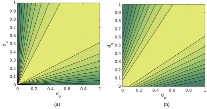
original measured(δp, δq) and our approximation corr(c(δp), c(δq)) is shown inFigure 5.

One clear difference is how small displacements are correlated. Whereas the original measure barely correlates small displacements, our approximation treats such displace-ments as similar, which seems more natural. If this is not intended, the functionfcan be tuned to suppress this correlation of low displacements. In particular, taking f (x) =xγ

allows us to discriminate more between small or large displacements, depending on the parameterγ.

4. Visual analytics for local analysis of delays

Varying the temporal scale in analyzing movement data is important to extract

move-ment patterns (Laube and Purves 2011). The global analysis of delays, discussed in

Section 3, enables to quantify whether and how much the trajectories are correlated.

To explore interaction events in detail, an approach over time and space on a local level is necessary.

In this section we summarize previous work (Konzacket al.2015) where a matching between the two trajectories was used to compute local movement patterns on a so-called delay space. To capture them in a visually salient way, we bundle edges as Figure 5.Comparison of displacements with our approximation. (a) Displacementsα= 2 (Long and Nelson2013). (b) Approximation usingβ= 0.15,f(dp) = 1 andgðdpÞ ¼π₂

logðdpþβÞ

log 1þ1 β

patches to indicate the source and relevance of the interaction event. Our focus lies on episodes of movement in which two moving entities show similar characteristics but possibly with a delay.

4.1. Requirements for analyzing interactions

The main analysis task concerns the interpretation of interaction events and patterns in two trajectories. Since interaction can be defined in different ways depending on the context, our visual analytics tool should allow the analyst to identify interaction pat-terns/events in the data for various interaction measures.

There can be many events, which may impede visual analysis if they are all shown in detail. The visualization should therefore allow an aggregation of the surroundings of a movement pattern to help an analyst focus on the progression of the interaction before and beyond the current event. This leads to the requirement that critical events should be visually salient.

Interaction of moving objects occurs at different scales: globally over the trajectories as a whole, locally at a specific point in time or over some time interval, or in episodes (a partitioning) of particular patterns (Laubeet al.2007). An analysis tool should therefore provide means to analyze interaction at different scales.

Our computational approach relies on determining a matching between the two trajectories in what we call a delay space. For the purpose of the analysis, it is necessary to understand the spatial structure of the delay space and its relation to the correspond-ing matchcorrespond-ing in space and time.

4.2. Computing matchings

To identify a potential interaction between the two moving entities, we are looking for pairs of data points, one from each trajectory, that are similar according to one of the distance measures discussed in Section 2. For this purpose, we first define the

delay space as a grid of distances for all pairs of points on the two trajectories (see

Figure 7(b)). More formally, given two trajectories with jτ1j ¼m and jτ2j ¼n, the delay space

DL:½1;m ½1;n !Rþ

is a grid ofm×npoints (pi, qj)∈T1× T2.

To identify delayed interactions, we compute a plausible alignment between the two trajectories. Such an alignment should map any point of one of the trajectories to another point on the other trajectory or to a contiguous range of points of the

other trajectory. We call such an alignment a matching between the trajectories. In

the delay space, this corresponds to a bi-monotone curve from the lower left corner (starting points of both trajectories) DL[1, 1] to the upper right (end points

of both trajectories) DL[m, n]. Such a matching is shown as a green curve in

Figure 7(b).

DTW aligns two trajectories–or more generally two time series–as to minimize the (squared) sum of distances between matched elements. The alignment can be com-puted in quadratic time using dynamic programming (Berndt and Clifford1994).

Theedit distance(ED) is a widely used measure for similarity between the two strings (Maier1978). It has been applied in bioinformatics and language processing. TheEDRis an adaption of ED for sequences with numerical values, for instance trajectories (Chen

et al.2005). The EDR tackles the problem of transforming numerical values into integer values from ED by defining a match on a pair of points. A pair of points is matched in EDR when the distance between the pair is less or equal to anεthreshold. To compute the EDR, a similar dynamic program as for DTW is used. The ε threshold restricts the choices within the dynamic program of EDR. DTW uses distances in the dynamic

program, whereas EDR uses unit costs. The longest common subsequence (LCSS) is

essentially a restricted version of the ED, where only two of the three operations of the ED are allowed (Wagner and Fischer1974).

Another alignment method minimizes the maximum distance along the trajectories. For curves, it is based on theFréchet distance, and the corresponding matching can be computed in near-quadratic time (Alt and Godau1995). More specifically, we use a

so-called locally correct Fréchet matching (LCFM). Such a matching has the following

property: if we take any subcurve of the matching (starting at a pair of time stamps (is, js) and ending at a pair (ie, je) and consider the subgrid of the delay space restricted to

the corresponding time stamps (DL :½is;ie ½js;je !Rþ), then an LCFM also

mini-mizes the maximum distance restricted to this subgrid (Buchinet al. 2012). Similar to this restriction, a profile function determines the structure of such a matching in a

lexicographic Fréchet matching (Rote 2014). In our tool we use the dynamic program-ming algorithm from Buchinet al. (2012) to compute such a discrete matching based on the Fréchet distance. The main idea is to construct a tree, with DL[1, 1] as the root, to all valid, subsequent and monotonous paths towards the root. All vertices on the path from DL[m, n] to the root are edges of the matching. This algorithm works with any premetric (seeSection 2) while Buchinet al. (2012) used it only with Euclidean distances.

To compute a matching on three or more trajectories, we need to extend the notion of a Fréchet matching from the two trajectories to a set of trajectories. Dumitrescu and Rote (2004) proposed a definition on the Fréchet distance on a set of curves. The Fréchet distance then is the longest leash in the set of curves, such that the length of the longest leash is minimized over all tuples of points from the input curves. Dumitrescu and Rote (2004) showed that a 2-approximation of the Fréchet distance on the set of curves can be constructed from all pairwise Fréchet distances.

Our visual analytics tool supports any of the alignment methods above and any similarity measures (seeSection 2), which allows to use a premetric in the delay space.

4.3. Interactive analysis of delays in matchings

The visual analytics approach allows users to explore matchings on two trajectories, the

degree of interaction and delays (Konzack et al. 2015). The proposed approach was

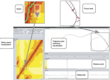
edges of a matching in colored patches. This makes changes of the delay visible over time, such that important local movement patterns can be perceived. A screen shot of the tool is shown inFigure 6.

The analytical process behind our visual analytics tool is the following:

(1) Open and load a data set

(2) Select a similarity measure and an alignment method (3) Analyze the structure of the matching

(4) Refine the parameters of the alignment method and the similarity measure (5) Identify interaction events by browsing the edges

First we need to open and load the data set of the moving objects into our visual analytics tool (step (1)). After that, we pick a similarity measure, used to construct the delay space, and an alignment method, which drives the structure of the computed matching (step (2)).

Upon that, we analyze the characteristics of the matching in the delay space and the trajectory visualization (step (3)) by navigating through the edges of the matching.

A matching enables an interactive, local analysis of delays by sliding through the edges of the matching. The main interaction component is the slider between the trajectory visualization and the distance plot, which browses the edges of the matching (not the time points), seeFigure 6.

A delay space is depicted inFigure 7(b). Trajectory B is on they-axis and trajectory R

on the x-axis. The values are shown by a linear heated body color scale, see e.g.,

Munzner (2014), and the matching is visualized as a green path through the delay

space. Diagonal line segments correspond to simultaneous movement of both objects, horizontal line segments correspond to movement of the object in R and stationary behavior in B, and vertical line segments correspond to movement in B and stationary behavior in R. In the delay space, seeFigure 6, a cursor points to the currently selected

edge of the matching–indices of the pair of points on the axes–accompanied by a

glyph to encode that trajectory B, symbolized by the blue triangle, is behind trajectory R –the red square (seeFigure 6for an enlargement). This stacking is swapped if trajectory B is ahead, and, if no delay occurs, both symbols appear side-by-side.

A monotonous matching has a nice property that has been used to simplify the visualization: in the matching, situations in which one point of one trajectory (the actor) is matched with several points of another trajectory (the reactor) occur often. This corresponds to an interaction pattern with a delayed response. These edges can be bundled into a single patch to avoid visual clutter. We color the patches to show the source, the actor, and the relevance of the corresponding reaction events.

An example visualization for two short trajectories, B and R, is shown inFigure 7(a). Trajectory B is below R, and reaction events of B and R are associated with the colors blue and red, respectively. Both moving entities start at the bottom of the plane, progress in the same direction, approach each other, split into almost opposite direc-tions and finally move in the same direction but at a large distance. The matching is based on the directional distance. At the beginning, there is almost no interaction, since both move along. The gray patch indicates a delayed response by R, where one point of B is matched to thefirst two points of R. As the moving objects approach each other, the structure of the patches becomes different. Within the red patch, the color changes from gray to red indicating that R increases the delay to B. The blue patch expresses that B reduces the delay to R until the delay vanishes (the color becomes gray).

The trajectory visualization, inFigure 6, provides an overview of all interactions over both trajectories in translucent colors. The selected edge and its direct surroundings in

the focus area are shown in saturated colors. The delay is visualized by glyphs: a circle for the actor and a red square or blue triangle for the reactor (the same visual encoding as in the delay space visualization). If no delay is observable, both points are depicted as circles.

As soon as we perceive the overall structure of the patches within the matching and its delay space as unfruitful, we refine the alignment method and/or the similarity measure (step (4)) such that we obtain a new delay space and a novel matching. For this new setting, we apply steps (2) to (4) until we are satisfied with the overall structure of the matching.

Eventually, we identify interaction events by browsing the edges of the matching (step (5)) in more detail. The aim is tofind consecutive episodes in both trajectories that correspond to high interaction. By tracing the patches in the form of action–reaction patterns in the trajectory visualization and rapid color changes in the delay space visualization, we are able to read off the time stamps for those events in the delay space visualization.

Additionally, the distance and delay plot, seeFigure 6, help to detect action–reaction patterns, which globally look as depicted in Figure 1, since significant changes in the progression of delays are related to changes in the interaction between the moving objects. The distance and delay plot show progression of distance and delay over time, respectively. The cursors help to read offexact values at the left side of the plots. The distances are also color-coded on a heated body color scale, and the delays are plotted in the colors of the trajectory.

5. Experiments

To evaluate our approach, we applied it on three data sets. First, we analyze the

interaction among the two ultimate Frisbee players (Long and Nelson 2013). On this

data set we compute global delays with our FFT-based approach on subsamples (episodes) to determine how well these episodes are correlated. Upon this, we analyze the covering performance between the attacker and the defender locally with our matching-based visual analytics tool.

The second data set is a pair of homing pigeons in collectiveflight (Pettitet al.2013). We are interested here in extracting interactive movement episodes by applying our visual analytics tool to a 2D projection of the moving pigeons.

On the third data set, a flock of homing pigeons (Santoset al.2014b), we selected three trajectories from the flock to analyze the interaction within a matching among these three moving objects. We compare the triplet matching with the pairwise match-ings on the three pigeons.

5.1. Analysis of the global delay on ultimate Frisbee data

The trajectories were simultaneously recorded with a sampling rate of 5 Hz, and each trajectory consists of 276 GPS locations. The duration of the recording is 60 s. Some missing locations occurred when the players were stationary. To resolve this issue, we interpolated the trajectories linearly over time for those missing locations. This inter-polated data set with 300 locations per trajectory has been used in our analysis.

Long and Nelson (2013) proposed a global measure for dynamic interaction to

determine whether there exists a substantial amount of interaction between the players. It is derived from the values from local dynamic interaction events. We compute a related measure, the global delay by using our FFT-based approach (seeSection 3).

We analyze the global interaction using displacements, since displacements are sensitive to the time shifts that are used for finding the global delay. This also allows us to evaluate the performance of approximations for displacements fromSection 3.2.

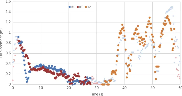
The main goal is to decide whether the trajectories have a substantial amount of interaction or not. To accomplish a distinction of interactive and noninteractive beha-vior, we selected subranges of the Frisbee data, such that we can perceive the difference in the global correlation among the trajectories. In Figure 8, the displacements of the two players are plotted over time. The selected subranges are indicated in saturated colors. We use the displacement measure withα= 1 throughout in this section. Wefirst compare the global delay between B1 and R1, then we compute the global delay between B1 and R2. To overlay the displacements, we shift the time stamps of R2 onto B1 by–30 s on each point of R2.

The set of trajectories B1 and R1, which we analyze for the global delay, are temporally aligned, and they consist of a significant amount of interaction within the

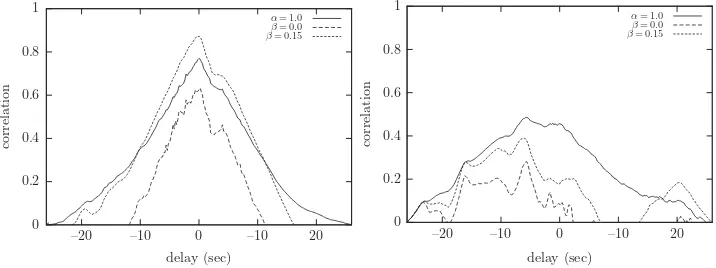
first 20 s (Long and Nelson 2013). In Figure 9(a) the correlation of displacements between B1 and R1 are computed for all possible time shifts and plotted as a black line. It is observable that the highest correlation is at 0 s, which is the global delay under

0 0.2 0.4 0.6 0.8 1 1.2 1.4 1.6

0 10 20 30 40 50 60

Displacement (m)

Time (s)

B1 R1 R2

the displacement similarity measure. Since either one or the other trajectory has been time-shifted for an alignment in the global delay, the plots for the global delay are asymmetrical. We also ran our FFT-based approach to approximate the displacements globally. The results are shown inFigure 9(a) for two values ofβas dashed lines (β= 0.0 and β= 0.15). It is observable that these values yield good approximations. However, there are some deviations at the boundaries of the time-shifting. The best

approxima-tion of displacements is when our FFT approach has aβbetween 0.0 and 0.15.

In the second set of trajectories B1 and R2 from Figure 8, we compare trajectories which are not temporally aligned. In order to compute a global delay between them, the

time stamps of R2 have been shifted by –30 s. The correlation of the displacements

between B1 and R2 is plotted in Figure 9(b) as a black line. There is not a remarkable correlation observable, and the maximum delay, the global delay, is not at 0 s. Our FFT approximations of the displacements, withβ= 0.0 andβ= 0.15, yield oscillating values (dashed lines). The correlations values are below the displacements, and we omitted negative values in the plot.

5.2. Analysis of delays on ultimate Frisbee data

In team sports, such as ultimate Frisbee, players engage in bursts of movement which may be characterized by different movement patterns. Therefore, a local analysis is more informative than a global analysis for the ultimate Frisbee data set (Long and Nelson

2013). Multiple episodes of different levels of interactions occur over time in this data set. Our aim is to segregate these segments into episodes of high and low interaction. To detect interaction events in our matching-based visual analytics tool, we need to choose a similarity measure (seeSection 2) for the delay space that captures the

move-ment pattern in a visual salient manner (step (2) in Section 4.3) and an alignment

method (see Section 4.2). In Figure 10(a–d), matchings have been computed for a

reaction pattern of the defender B to the attacker R (step (4)). We used, as Long and Nelson (2013), anα= 1 in the dynamic interaction measure. The loop and its adjustment between the players afterwards are captured clearly in matchings based on the

α=1.0

β=0.0

β=0.15

α=1.0

β=0.0

β=0.15

–20 –10 0 –10

delay (sec) 20 –20 correlation 0.2 0.4 0.6 0.8 1 0 correlation 0.2 0.4 0.6 0.8 1 0

–10 0 –10

delay (sec)

20

Euclidean distance and the directional distance. As alignment method we first use an LCFM.

We opt for analyzing the ultimate Frisbee data set under the directional distance, since this delay space is sensitive to direction-based and spatial properties. Within the

episodes 0–25 s and 36–45 s, both players have a low distance, meaning a high

interaction. This is consistent with thefindings of Long and Nelson (2013). Our measures detect an additional episode of interaction: Within the interval 45–57 s, a turn by R is followed by a reaction of B, seeFigure 10.

The progression of the distance over time, seeFigure 11(a), follows the structure of an action-reaction pattern, discussed in the previous section. In the delay plot, this event can also be seen in the form of a significant change of the local delay, seeFigure 11(b). Long and Nelson (2013) analyzed the covering performance by the dynamic interaction measure on pairs of points with the same time stamp, which is why our notion of delay therefore does not occur in their analysis.

Next we performed the same analysis but with different alignment methods,

speci-fically DTW and EDR. We computed matchings on the two trajectories using DTW and

EDR. These algorithms have the same running time ofO(n2) as computing an LCFM. In the dynamic programs for DTW and EDR, we maintained predecessor graphs to Figure 10.Matchings under different similarity measures to detect a loop pattern in the ultimate Frisbee data: (a) based on the Euclidean distance measure, (b) based on the similarity of headings, (c) based on the dynamic interaction similarity measure, and (d) based on the directional distance similarity measure. (a) highlights it as an interaction event. For (b) in the delay space, only the adjustment of the defender B towards the attacker R is found, since it highlights the loop pattern partially as two patches. Using the dynamic interaction measure in the delay space (c) yields three patches, but the adjustments of the defender after the loop are not captured as separate events. (a) and (d) highlight the loop as an interaction event by a blue patch followed some smaller patches during the adjustments within the reaction of the defender B.

construct a matching and not only compute the distance value. The original definition of EDR uses an epsilon on the absolute difference on each dimension of a pair of points. However, we used anεthreshold on the actual distance norm used in the delay space to match a pair of points.

InFigure 12, we computed matchings in the delay space using the Euclidean distance

for the loop pattern of the ultimate Frisbee data. The horizontal stripe in the matchings of all the three methods corresponds to the reaction movement of the defender. All methods capture the loop. EDR recognizes the loop premature with respect to other methods over time. The progression of the matching curve in DTW and EDR are some-how similar. However, an LCFM consists of more vertical segments in the matching than DTW and EDR. Hence the LCFM has more bends to move through regions with low distances in the delay space, whereas the matchings based on DTW and EDR tend to stay shorter in this area of low distances.

The threshold parameterεto match a pair of points influences heavily the structure of a matching based on EDR. A relatively large or low value forces the matching to prefer diagonal movements in the delay space. A preanalysis of distribution of the distances that may occur in a possible matching need to be conducted in order to spot a suitableεvalue, since a relatively large or low value forεforces the matching to prefer diagonal movements even when there are vertical or horizontal movements with lower distances possible to take. Hence, EDR suffers from spotting an appropriateεbefore computing a matching, whereas other techniques give better results without a need of a parameter at all.

5.3. Analysis of delays on pigeon data

et al. (2013). The time span of the data is 140 s using a sampling rate of 5 Hz. The trajectories have not been tuned or optimized. Pigeon Bflies a distance 1.62 km at an average speed of 16.75 ± 5.02 ms–1to land 634 m from its start point, and pigeon Rflies 1.33 km at an average speed of 15.36 ± 4.92 ms–1to land a distance 572 m from its start point. In this analysis we used directional distance in combination with LCFM.

An overview visualization is shown inFigure 13for a selected event, where pigeon R reacts to the movement of pigeon B. The reaction of pigeon R is a transition from a right

turn to a left turn. This event is visible as a large blue patch inFigure 13(b). In the delay space, see Figure 13(a), this movement pattern is indicated by the horizontal segment within the matching. Due to the adjustment of pigeon R to the movement of pigeon B as a reaction, there is a decline in the distance, seeFigure 13(d). The delay still increases at this point until the maximum delay is reached within the reaction movement of pigeon R, seeFigure 13(e). The movements of the pigeons and its matching visualization are outlined inFigure 13(c), and only the surroundings of the selected edge are in the focus of the visualization.

Within 0–12 s and 20–66 s, the pigeons have low directional distance, indicating high interaction, as can be seen in both the distance plot and delay plot (seeFigure 13). The delay plot indicates that the leadership switches between these two episodes. The directional distance then increases, but from 95 s to 106 s and starting from 120 s, the pigeons have high interaction again. Between 106 s and 120 s, one pigeon makes a loop while the other progresses in a straight line.

To evaluate these findings informally with those from another technique, we

applied the time-ordering approach by Giuggioliet al. (2015) on the pigeon data set,

seeFigure 14. For this approach we have focused on the velocity cross-correlation to

identify and classify copying patterns in direction. The optimal movement episodes, based on a directional separation, are similar to the episodes detected by our approach. For computational convenience the maximum allowed delays were capped at 4.5 s.

The episodes 0–18 s, 20–65 s, and 120–130 s are consistent with those from our approach. At around 105 s and 118 s, two short movement episodes of interactive behavior have been found. They capture the beginning and the end of the loop pattern, but it is not detected as a whole. The deviations are probably due to the delay parameters of the time-ordering approach, since in our matching-based approach quite large delays (max. 9.6 s) occur at around 120 s.

When compared to the time-ordering procedure the present approach has various advantages. It does not require a presmoothing of the data set, and it can be extended beyond pairwise analysis.

5.4. Analysis of delays on a triplet of pigeons

Our approach focused so far on the analysis of interaction on two trajectories. However, it is common in applications to track several moving object as a collective movement, such as aflock or a group. A procedure to analyze the interaction among more than two trajectories simultaneously is in fact very much in need.

There are two reasons why a pairwise procedure on more than two trajectories is likely to fail: one is practical and the other methodological. The practical aspect is that the computational cost increases very rapidly if one accounts for all possible pairs of trajectories. The methodological problem is due to potential inconsistencies in identify-ing the correct sequence of events. To explain it, let us consider the example of three simultaneously moving objects, A, B, and C. Suppose that a pairwise procedure between A and B and between A and C indicates, respectively, that B reacts to A with a (positive) delayτBA, and that C reacts to A with a (positive) delayτCA>τBA. IfτBAis quite different

fromτCA, the pairwise analysis between B and C most likely will extract a delayτCB> 0,

consistent with the fact that individual C has responded to individual A later than individual B. But if the pairwise delays extracted are small, then it is not ensured that τCB> 0. To avoid these issues, one ought to extract delay for all individuals at once.

To do so, we extend our approach to compute a matching on three simultaneously moving objects, and we compare how the triplet analysis differs from a pairwise analysis and how well a triplet matching captures action–reaction patterns on a local scale.

We use a data set of aflock of 10 pigeons from Santoset al. (2014b), which has been made available on Movebank (Santoset al.2014a). It consists of simultaneously recorded GPS data using a sampling rate of 4 Hz. The pigeons have been tracked for several trips. All pigeons from theflock are likely to interact with each of the others, since they are socially familiar to each other (Santoset al.2014b). The transitive, pairwise comparison of the pigeons in Santoset al. (2014b) has shown results with significant repeatability, such that we can validate the pairwise matchings with that one obtained directly from the triple.

We have selected three trajectories, pigeon M, S, and U, corresponding to different roles within theflock. Pigeon M has high rank for leadership, and pigeons S and U have

low negative leadership rank within the flock. Pigeons S and U are likely to show

follower behavior. Santos et al. (2014b) explain that leadership has a stable role within aflock across differentflights.

A pairwise matching between pigeon M and S is shown in Figure 6. It captures a

position, heading, and turns occur. Within the beginning of a flight, there are many

adjustments among the pigeons to the collective movement of theflock, which is why

we use a sample of 200 points fromflight 5 from time stamps 800 to 999, whereasflight 5 consists of 3845 time-stamped points in total.

To measure similarity between a triple of points, we used the maximum of the pairwise Euclidean distance (seeSection 2) in our methods, LCFM and DTW, to compute a triplet matching. For the pairwise analysis, we used the Euclidean distance on the selected pair of trajectories.

We projected the triplet matching into our visual analytics tool by showing only the coordinates of the selected pair and leaving out the values of the nonselected trajectory. An LCFM on a triplet results in a similar matching as a pairwise computation on the three trajectories separately. This can be seen in Figure 15. A pairwise matching is visualized as a blue curve in the delay space and the projected triplet matching in green. The triplet matching on the pair (S, U) coincides with the LCFM on that pair of trajectories. The S-shape of the delay space is due to a sharp turn by S within the circular, anticlockwise movement of theflock. The longest leash is from the pair (S, U),

since this projection (see Figure 15) of the triple matching moves through a short

segment within the S-turn in the brightest color of all three projections. Hereby it contains the largest Euclidean distance of the triplet matching. The longest leash gives the pairs (M, S) and (M, U) slack for their edges within the triplet matching. This fact is likely to explain why the pairwise projections deviate by having horizontal stripes in the triplet matching. However, these projections still avoid large values in the delay space.

To evaluate this LCFM on a triple of trajectories, we have computed a triplet matching

based on DTW. Figure 16shows the projections in green and beneath it the LCFM on

the selected pair in blue. The projections for the pairs (M, U) and (S, U) follow the progression of the pairwise LCFM. The triplet matching on the pair (M, S) clearly deviates from the LCFM, since it prefers diagonal movement in the delay space. This can be explained by the fact that DTW optimizes the squared sum of Euclidean distances. As a result, it prefers to minimize large distance values. The pairs (M, U) and (S, U) preserve a significantly large distance with respect to (M, S).

Overall the matchings between triplets provide results similar to those obtained by pairwise matchings. Although in general such equality may not be ensured as we explained earlier, for this data set it holds true independently of the alignment method used (DTW or LCFM).

6. Conclusions

We proposed a new approach to analyze interaction events between the two trajec-tories. First, we determine with our FFT-based approach whether there is any interaction between the trajectories. Upon that, we apply our main technique on the data set, a versatile visual analytics tool which enables time delays to be incorporated in interaction movement analysis.

structure of the interaction events. The relevance of the movement pattern is determined by the delay among the moving entities, which is used as a color saturation for the patches.

The experiments show that the structure of a matching provides important insights

into action–reaction patterns in the movement data. The computation of a matching

relies on the alignment method. We evaluated various types of state-of-the-art methods to compute a matching. All of them are supported in our visual analytics tool. In general, DTW and LCFM gave good results in our experiments. If the movement of trajectories is relatively aligned, then DTW and LCFM yielded both good results. However, LCFM gives better alignments as soon as delayed responses appear within the movement data, since DTW tends to prefer diagonal movements in the delay space.

We surveyed various interaction measures in our tool as well, which combine move-ment vectors, distance norm, or headings of the trajectories. By combining the Euclidean distance norm and the difference in the headings, we introduced the novel premetric, the directional distance. In our experiments using the directional distance yields large patches, e.g., in the loop movement of the ultimate Frisbee data set, with respect to other similarity measures, capturing action–reaction relationships better as visible colored patches in the visual analytics tool.

The concept of a delay space and a matching can be generalized to more than two trajectories. We showed this on a triplet of trajectories. In the experiments, the results on the triplet were consistent with those from a pairwise analysis. They did not provide additional insights to our data sets, however.

Visualizing the delay space and matching between simultaneously moving objects is challenging, since the delay space then has at least three dimensions. Our delay space visualization is limited to support only two trajectories as x- and y-axes. Therefore, a novel technique needs to be developed to visualize a matching on more than two trajectories. Beyond the examples presented in our experiments, our methods are widely applicable to analysis of individual human movement in a crowd, prey–predator inter-action, wilding mating behavior, and sports analysis.

Acknowledgments

We thank Georgina Wilcox and Joachim Gudmundsson for their initial idea work on the delay space and proofreading this article. Maximilian Konzack, Tim Ophelders, Michel A. Westenberg and Kevin Buchin are supported by the Netherlands Organisation for Scientific Research (NWO) under grant no. 612.001.207 (Maximilian Konzack, Michel A. Westenberg and Kevin Buchin) and grant no. 639.023.208 (Tim Ophelders).

Disclosure statement

No potential conflict of interest was reported by the authors.

Funding

ORCID

Jed Long http://orcid.org/0000-0003-3961-3085

References

Alt, H. and Godau, M., 1995. Computing the Fréchet distance between two polygonal curves.

International Journal of Computational Geometry & Applications, 5 (1–2), 78–99. doi:10.1142/ S0218195995000064

Andrienko, N.,et al.,2013. Space transformation for understanding group movement.IEEE Transactions on Visualization and Computer Graphics, 19 (12), 2169–2178. doi:10.1109/TVCG.2013.193

Berndt, D.J. and Clifford, J.,1994. Using dynamic time warping tofind patterns in time series.In:

KDD workshop. Vol. 10, Seattle, WA, 359–370.

Brigham, E.O.,1988.The fast Fourier transform and its applications. Upper Saddle River, NJ: Prentice Hall.

Buchin, K., Buchin, M., and Gudmundsson, J.,2008. Detecting singlefile movement.In:Proc. 16th ACM SIGSPATIAL International Conference on Advances in Geographic Information Systems (ACM GIS), Irvine, CA, 288–297.

Buchin, K.,et al.,2012. Locally correct Fréchet matchings.In:Algorithms–ESA 2012. Berlin: Springer, 229–240.

Chen, L., Özsu, M.T., and Oria, V., 2005. Robust and fast similarity search for moving object trajectories.In:Proceedings of the 2005 ACM SIGMOD international conference on Management of data, Baltimore, MD, 491–502.

Doncaster, C.P.,1990. Non-parametric estimates of interaction from radio-tracking data.Journal of Theoretical Biology, 143 (4), 431–443. doi:10.1016/S0022-5193(05)80020-7

Dumitrescu, A. and Rote, G., 2004. On the Fréchet distance of a set of curves. In: Canadian Conference on Computational Geometry (CCCG), Montréal, 162–165.

Giuggioli, L., McKetterick, T.J., and Holderied, M.,2015. Delayed response and biosonar perception explain movement coordination in trawling bats.PLOS Computational Biology, 11 (3), e1004089. doi:10.1371/journal.pcbi.1004089

Kareiva, P. and Shigesada, N., 1983. Analyzing insect movement as a correlated random walk.

Oecologia, 56 (2–3), 234–238. doi:10.1007/BF00379695

Konzack, M., et al.,2015. Analyzing delays in trajectories. In: Proc. 8th IEEE Pacific Visualization Symposium (PacificVis 2015), Hangzhou, 93–97.

Laube, P.,et al., 2007. Movement beyond the snapshot—dynamic analysis of geospatial lifelines.

Computers, Environment and Urban Systems, 31, 481–501. doi:10.1016/j.compenvurbsys.2007.08.002 Laube, P. and Purves, R.S., 2011. How fast is a cow? Cross-scale analysis of movement data.

Transactions in GIS, 15 (3), 401–418. doi:10.1111/j.1467-9671.2011.01256.x

Long, J.A. and Nelson, T.A.,2013. Measuring dynamic interaction in movement data.Transactions in GIS, 17 (1), 62–77. doi:10.1111/tgis.2013.17.issue-1

Maier, D.,1978. The complexity of some problems on subsequences and supersequences.Journal of the ACM (JACM), 25 (2), 322–336. doi:10.1145/322063.322075

Merki, M. and Laube, P., 2012. Detecting reaction movement patterns in trajectory data. In:

Proceedings of the AGILE 2012 International Conference on Geographic Information Science, Avignon, 25–27.

Munzner, T.,2014.Visualization analysis and design. Boca Raton, FL: CRC Press.

Nagy, M.,et al.,2010. Hierarchical group dynamics in pigeonflocks.Nature, 464 (7290), 890–893. doi:10.1038/nature08891

Pettit, B.,et al.,2013. Interaction rules underlying group decisions in homing pigeons.Journal of The Royal Society Interface, 10 (89), 20130529. doi:10.1098/rsif.2013.0529

Rote, G.,2014.Lexicographic Fréchet Matchings. Technical report, EuroCG 2014.

Santos, C.D.,et al.,2014a. Data from: Temporal and contextual consistency of leadership in homing pigeonflocks.Movebank Data Repository. doi:10.5441/001/1.33159h1h

Santos, C.D.,et al.,2014b. Temporal and contextual consistency of leadership in homing pigeon flocks.PloS one, 9 (7), e102771. doi:10.1371/journal.pone.0102771