Declining Vegetation Growth Rates in the Eastern United States from 2000 to 2010

Declining Vegetation Growth Rates in the Eastern United

States from 2000 to 2010

Christopher Potter1*, Shuang Li1,2, Cyrus Hiatt1,2

1_{NASA Ames Research Center, Moffett Field, USA;} 2_{California State University Monterey Bay, Seaside, USA.}

Email: *_{[email protected]}

Received July 20th_{, 2012; revised September 6}th_{, 2012; accepted September 18}th_{, 2012}

ABSTRACT

Negative trends in the monthly MODerate resolution Imaging Spectroradiometer (MODIS) Enhanced Vegetation Index (EVI) time-series were found to be widespread in natural (non-cropland) ecosystems of the eastern United States from 2000 to 2010. Four sub-regions were detected with significant declines in summed growing season (May-September) EVI, namely the Upper Great Lakes, the Southern Appalachian, the Mid-Atlantic, and the southeastern Coastal Plain forests ecosystems. More than 20% of the undeveloped ecosystem areas in the four sub-regions with significant nega- tive EVI growing season trends were classified as forested land cover over the entire study period. We detected rela- tionships between annual temperature and precipitation patterns and negative forest EVI trends across these regions. Change patterns in both the climate moisture index (CMI) and growing degree days (GDD) were associated with de- clining forest EVI growing season trends. We conclude that temperature warming-induced change and variability of precipitation at local and regional scales may have altered the growth trends of large forested areas of the eastern United States over the past decade.

Keywords: MODIS EVI; Forest; Growth; Climate Change; United States

1. Introduction

There is considerable uncertainty about changing growth rates of forests in the eastern United States. Based on a small number of field site measurements, forest biomass accumulation was reported to be accelerating in the re- gion at locations where nutrients and water were not lim-iting [1,2]. At the same time, reduction of wildfire through- out the eastern US has evidently converted more lands to closed-canopy forests with more shade-tolerant, fire-sen- sitive plants [3].

Standing in contrast to these results are a number of recent climate change impact studies on the region. Over the last century, the eastern US has become warmer, par- ticularly since 1970 at the rate of 0.45˚F per decade [4]. Outbreaks of insect pests and introduced pathogens have become dominant forces driving changes in forests of the eastern US [5].

The effects of longer vegetation growing seasons and periodic drought on US plant production have been re-ported [6,7]. [8] further examined changing soil freeze- thaw signal from satellite microwave remote sensing and vegetation greenness patterns for the 9-year (2000-2008) vegetation record from satellites over North America,

and reported that the relationship between the non-frozen period (Jun-Aug) and mean summer greenness index anomalies was generally positive for tundra and boreal forests areas of Canada, but was negative for temperate forest areas of the eastern US, for which they suggested that moisture availability was a critical control on annual forest growth patterns.

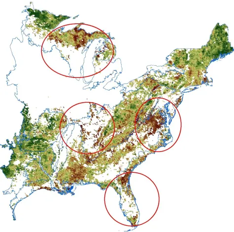
Satellite remote sensing has been shown to be an ac-curate method to monitor large-scale regrowth of green vegetation cover and productivity, especially following disturbance [9-12]. In this study, we utilized over ten years of the MODerate resolution Imaging Spectroradio- meter (MODIS) Enhanced Vegetation Index (EVI) satel- lite data to examine the relationships between natural (non- developed) vegetation growth trends and climate indices in ecosystems of the eastern US. The study area covered all of the eastern United States over the time period from 2000 to 2010 (Figure 1).

2. Methods

Collection 5 MODIS data sets beginning in the year 2000 were obtained from NASA’s Land Processes Distributed Active Archive Center site [13]. MODIS EVI values were aggregated to 8-km resolution from MOD13C2 (MODIS/Terra Vegetation Indices) products. MOD13C2

Figure 1. Slope of the time-based (2000-2010) EVI regression in natural ecosystem areas of the eastern US region. Green shades indicate a positive slope of increasing growing season EVI, whereas brown shades indicate a negative slope of de-creasing growing season EVI. Four general sub-regions listed in Table 1 are identified in red lines and were delineated for analysis according to Major Land Resource Areas (MLRAs, source: US geological survey and the natural resources con- servation service, USDA) shown in blue lines.

data are cloud-free spatial composites of the gridded 16- day 1-kilometer MOD13A2 product, and were provided monthly as a level-3 product projected on a 0.05 degree (5600-meter) geographic Climate Modeling Grid (CMG). Cloud-free global coverage at 8-km spatial resolution was achieved by replacing clouds with the historical MODIS time-series EVI record. MODIS EVI was calculated from red, blue and NIR bands as described by [14]. Monthly EVI values were summed across each six-month grow-

ing season period (May through September) to represent the variability in vegetation productivity for the past 11 years.

2009 were aggregated to 8-km resolution and compared for vegetation change detection and exclusion of non- natural (e.g., developed as cropland or urban) ecosystem areas from the analysis. PRISM (Parameter-elevation Re- gressions on Independent Slopes Model) data sets were used for precipitation, average maximum temperature, and average minimum temperature [17]. These 4-km cli- matologies were derived from US weather stations re- cords interpolated first into 30 arc-second data sets. PRISM is unique in that it incorporates a spatial knowledge base that accounts for topographic influences such as rain sha- dows, temperature inversions, and coastal effects, in the climate mapping process.

Monthly potential evapotranspiration (PET) from global sources [7] were also prepared for analysis. Annual cli- mate indexes for each year 2000-2010 were calculated from these monthly meteorological datasets to use as in- dependent explanatory variables. The climate index se- lection was based on previous study results from [18], which showed that degree days, annual precipitation to- tals, and an annual moisture index together can account to 70% - 80% of the geographical variation in the global vegetation seasonal extremes. Selected indexes in this study included: the climate moisture index (CMI, [19]) and growing degree days (GDD) base 0˚C. The CMI indicator ranges from –1 to +1, with negative values for relatively dry years, and positive values for relatively wet years. GDD is the number of days for which mean monthly temperature was greater than 0˚C.

According to the values of the slope and the coeffi- cient of determination (R2) of the EVI time-based re-

gressions, all ecosystem pixels were classified into one of three categories: 1) Pixels with a positive trend, where Slope > 0 and a 95% level of significance for a two-tailed t-test (R2≥ 0.37); 2) Pixels with a negative trend with a

95% level of significance (where Slope < 0 and R2 ≥

0.37); 3) Pixels with a non-significant trend (R2 < 0.37,

Slope > 0, or Slope < 0). The “Breaks for Additive Sea- sonal and Trend” method (BFAST, [20,21]) was further applied to the EVI monthly time series for annual trend characterization. [22] analyzed trends in normalized dif- ference vegetation index (NDVI) satellite data between 1982 and 2008 using the BFAST procedure and detected both abrupt and gradual changes in large parts of the

world, especially in (semi-arid) shrubland and grassland biomes where abrupt greening was often followed by gra- dual browning.

3. Results and Discussion

Significant negative EVI trends were found to be wide- spread in natural ecosystems of the eastern US from 2000 to 2010 (Figure 1). Four sub-regions were identified with

extensive areas of decline in growing season EVI, namely the Upper (northwestern) Great Lakes, the Southern Ap- palachian, the Mid-Atlantic, and the southeastern Coastal Plain ecosystems. A range of 13% (northwestern Great Lakes and Southern Appalachian) to 47% (Mid-Atlantic) of unburned ecosystem area in the four sub-regions of the eastern US was detected with significant negative EVI trends over the study period (Table 1). Out of the four

sub-regions, only the southeastern Coastal Plain (with >10% burned area within the significant negative EVI trend category) was partially impacted by wildfires at a frequency of more than 1% of the total natural (forest and shrubland) area burned. Overall, 17% of all ecosys- tem areas (and 10% of all forest areas) in the four sub- regions were detected with significant negative EVI trends over the study period. Only the northwestern Great Lakes sub-region was detected as having a notable (1.6%) area coverage with significant positive EVI trends over the study period (Table 1), none of which could be at-

tributed to regrowth following forest fires.

Approximately 21% of the total natural ecosystem ar-eas in the four sub-regions with significant negative EVI trends were classified as forested land cover over the entire study period. This predominant (and unburned be- tween 2000 and 2010) forest area with significant nega- tive EVI trend totaled 32,576 km2_{, based on a compari-}

son of 500-m MODIS land cover from 2001 to 2009 (Table 2). More than one-half of this total unburned for-

est area with significant negative EVI trends in the four sub-regions was located in the Upper Great Lakes sub-region (Table 3). It is also worth noting that nearly

40% of the total forest area within the Mid Atlantic sub- region showed significant negative EVI trends. Because land cover classification did not change in these forest

Table 1. Area (in km2) of growing season EVI trends in sub-regions of the eastern US over the period 2000-2010.

Sub-Region Sig. Positive Sig. Negative Non-Significant Total % Sig. Negative

Upper Great Lakes 13,568 38,272 241,664 293,504 13.0

Mid Atlantic 0 23,168 25,920 49,088 47.2

Southern Appalachian 896 58,432 374,976 434,304 13.5

Southeastern Coastal Plain 256 29,568 68,736 98,560 30.0

Table 2. Land cover change confusion matrix for 8-km pixel areas aggregated from 500-m MODIS cover classes for 2001 and 2009 determined by >75% majority coverage in the four sub-regions shown in Table 1.

Class 2009 Class 2001 Water Forest Grass-Savanna Developed1 _Mixed2

Water 16 0 0 0 0

Forest 0 4743 2 0 190

Grass-Savanna 0 0 5 0 16

Developed 0 0 0 1574 425

Mixed 2 1237 5 85 5379

1_{Included cropland and urban cover classes;} 2_{Composed of a mixture of the other three cover classes with not single class representing >75% majority coverage.}

Table 3. Area of significant negative growing season EVI trends in forests sub-regions of the eastern US over the period 2000-2010.

Sub-Region Sig. Negative EVI Forest Area (km2_{) % Forest Area with Sig. Negative EVI}

Upper Great Lakes 17,472 14

Mid Atlantic 3456 38

Southern Appalachian 9408 6

Southeastern Coastal Plain 2240 12

Total 32,576 10

areas over the EVI analysis study period of 2000 to 2010, we hypothesized that the consistent decline in growing season EVI must be attributed to climate-related factors.

Break point analysis on forest areas with significant negative EVI trends in the region revealed that nearly 63% of all negative trend areas in the four sub-regions had zero break points, which indicated that growth rates declined gradually and consistently during the MODIS observation period (2000-2010). The other 37% (Table 4)

of all negative trend areas detected with one or more break point over past decade appear to have had vegeta- tion growth abruptly interrupted by some external factor (e.g., extreme weather events, insect damage), leading to a sudden decline in growing season EVI.

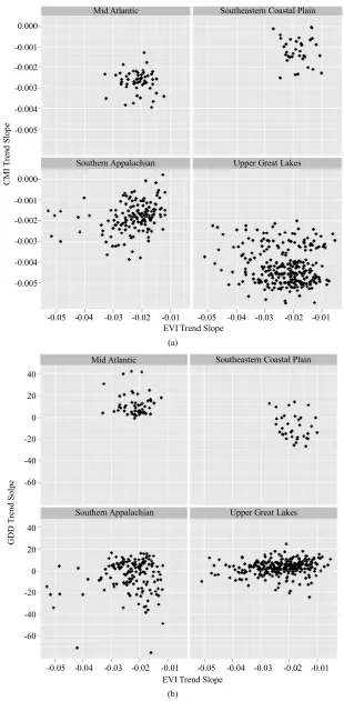
A strong association was observed between the slope of annual CMI and negative EVI trends (Figure 2(a)).

Nearly all the forest areas in the four sub-regions of the eastern US detected with significant negative EVI trends were associated with relative drying trends (i.e., strongly

negative CMI slope values). The Upper Great Lakes re- gion showed the strongest association between negative annual CMI and negative growing season EVI trends. These results suggest that dry years in this sub-region are closely related to declines in forest growth as detected by trends in summer-time EVI.

Positive slope values of GDD (base 0˚C) indicated a warming trend over the past decade. There were strong associations between positive GDD slopes and negative growing season EVI slopes in all the four sub-regions, and particularly in the Mid-Atlantic and the southeastern Coastal Plain forest areas (Figure 2(b)). The Southern

Table 4. Percentage categories from the BFAST break point analysis for forest sub-regions of the eastern US with sig-nificant negative EVI trends from 2000-2010.

Zero Break

Points 1 Break Point 2 Break Points Greater than 2 Break Points

62.5% 26.5% 8.4% 2.6%

Appalachian sub-region showed the weakest associations between negative forest EVI trends and either CMI or GDD (drying or warming, respectively) trends over the period 2000 to 2010. We postulate that the complex to- pography, hydrology, and variable elevation zones of moun- tainous areas in the Appalachian region can confound association analysis of climate trends with EVI trends, at least more so than within the other sub-regions.

4. Conclusions

The MODIS EVI time-series data used in this study pro- vided consistent large-scale metrics of forest growth trends across the eastern US region. Temperature warming-in- duced change and inter-annual variability of precipitation at local and regional scales may have altered the trends of large forest growth and could be impacting the resil- ience of forest ecosystems across certain sub-regions.

-0.05 -0.04 -0.03 -0.02 -0.01 -0.05 -0.04 -0.03 -0.02 -0.01 EVI Trend Slope

Southern Appalachian 0.000

-0.001

-0.002

-0.003

-0.004

-0.005

0.000

-0.001

-0.002

-0.003

-0.004

-0.005

CMI

T

re

nd

Sl

op

e

Upper Great Lakes Mid Atlantic Southeastern Coastal Plain

(a)

-0.05 -0.04 -0.03 -0.02 -0.01 -0.05 -0.04 -0.03 -0.02 -0.01 EVI Trend Slope

Mid Atlantic Southeastern Coastal Plain 40

20

0

-20

-40

-60

40

20

0

-20

-40

-60

GDD T

re

nd

Sol

pe

Southern Appalachian Upper Great Lakes

(b)

to a small decline (0.001 - 0.004 yr - 1; 5% overall be- tween 2002 and 2010) in NDVI under a range of simu-lated aerosol conditions and high-latitude surface types. Similar evaluations have not yet been conducted for sen- sor degradation impacts on MODIS EVI in mid-latitudes, such as the eastern US region in this study (D. Wang, personal communication), but we can add that over half of the forest areas detected with a decline in growing season EVI in our results above (Tables 3 and 4) ex-

ceeded 6% overall between 2000 and 2010 and the de- cline was frequently not gradual, such as could be attrib- uted to MODIS sensor degradation.

In summary, the methodology developed for mapping and characterization of forest growth trends can be read- ily extended over the next decade of Collection 6 MODIS EVI data. The results from BFAST break point analysis provides an additional trend decomposition method for local scale studies with higher resolution satellite data. Further research should be pursued in order to elucidate the developing relationship between forest growth de- cline and climate change in the eastern US region.

5. Acknowledgements

This work was conducted with the support from NASA under the US National Climate Assessment. This re- search was also supported by an appointment of the sec- ond author to the NASA Postdoctoral Program at the NASA Ames Research Center, administered by Oak Ridge Associated Universities. We thank Vanessa Genovese, and Steven Klooster of California State University Mon- terey Bay for assistance with regional data sets and pro- gramming.

REFERENCES

[1] C. Boisvenue and S. W. Running, “Impacts of Climate Change on Natural Forest Productivity—Evidence Since the Middle of the 20th Century,” Global Change Biology,

Vol. 12, No. 5, 2006, pp. 1-21. doi:10.1111/j.1365-2486.2006.01134.x

[2] S. McMahon, G. Parker and D. Miller, “Evidence for a Recent Increase in Forest Growth,” Proceedings of the

National Academy of Sciences, Vol. 107, No. 8, 2010, pp.

3611-3615. doi:10.1073/pnas.0912376107

[3] G. J. Nowacki and M. D. Abrams, “The Demise of Fire and ‘Mesophication’ of Forests in the Eastern United States,”

BioScience, Vol. 58, No. 2, 2008, pp. 123-138.

doi:10.1641/B580207

[4] K. Hayhoe, C. P. Wake, T. G. Huntington, L. Luo, M. D. Schwartz, J. Sheffield, E. Wood, B. Anderson, J. Brad- bury, A. DeGaetano, T. J. Troy and D. Wolfe, “Past and Future Changes in Climate and Hydrological Indicators in the US Northeast,” Climate Dynamics, Vol. 28, No. 4,

2007, pp. 381-407. doi:10.1007/s00382-006-0187-8 [5] G. M. Lovett, C. D. Canham, M. A. Arthur, K. C. Weathers

and R. D. Fitzhugh, “Forest Ecosystem Responses to Ex- otic Pests and Pathogens in Eastern North America,” Bio-

Science, Vol. 56, No. 5, 2006, pp. 395-405.

doi:10.1641/0006-3568(2006)056[0395:FERTEP]2.0.CO; 2

[6] R. B. Myneni, C. D. Keeling, C. J. Tucker, G. Asrar and R. R. Nemani, “Increased Plant Growth in the Northern High Latitudes from 1981 to 1991,” Nature, Vol. 386, No.

6626, 1997, pp. 698-702. doi:10.1038/386698a0

[7] C. Potter, S. Klooster and V. Genovese, “Net Primary Production of Terrestrial Ecosystems from 2000 to 2009,”

Climatic Change, Vol. 115, No. 2, 2012, pp. 365-378.

doi:10.1007/s10584-012-0460-2

[8] Y. Kim, J. S. Kimball, K. Zhang and K. C. McDonald, “Satellite Detection of Increasing Northern Hemisphere Non-Frozen Seasons from 1979 to 2008: Implications for Regional Vegetation Growth,” Remote Sensing of Environ- ment, Vol. 121, 2012, pp. 472-487.

doi:10.1016/j.rse.2012.02.014

[9] B. D. Amiro, J. M. Chen and J. Liu, “Net Primary Pro- ductivity Following Forest Fire for Canadian Ecoregions,”

Canadian Journal of Forest Research, Vol. 30, No. 6,

2000, pp. 939-947. doi:10.1139/x00-025

[10] J. Epting and D. L. Verbyla, “Landscape Level Inter- actions of Pre-Fire Vegetation, Burn Severity, and Post- Fire Vegetation over a 16-Year Period in Interior Alaska,”

Canadian Journal of Forest Research, Vol. 35, No. 6,

2005, pp. 1367-1377. doi:10.1139/x05-060

[11] M. Cuevas-GonzALez, F. Gerard, H. Balzter and D. Ri-aNO, “Analysing Forest Recovery after Wildfire Distur- bance in Boreal Siberia Using Remotely Sensed Vegeta- tion Indices,” Global Change Biology, Vol. 15, No. 3, 2009,

pp. 561-577. doi:10.1111/j.1365-2486.2008.01784.x [12] G. M. Casady and S. E. Marsh, “Broad-Scale Environ-

mental Conditions Responsible for Post-Fire Vegetation Dynamics,” Remote Sensing, Vol. 2, No. 12, 2010, pp. 2643-

2664. doi:10.3390/rs2122643

[13] LP-DACC: NASA Land Processes Distributed Active Archive Center, “MODIS/Terra Vegetation Indices Monthly L3 Global 0.05Deg CMG (MOD13C2),” 5th Edition, USGS/Earth Resources Observation and Science (EROS) Center, Sioux Falls, 2007.

[14] A. Huete, K. Didan, T. Miura, E. Rodriquez, X. Gao and L. Ferreira, “Overview of the Radiometric and Biophy- sical Performance of the MODIS Vegetation Indices,” Re-

mote Sensing of Environment, Vol. 83, No. 1-2, 2002, pp.

195-213. doi:10.1016/S0034-4257(02)00096-2 [15] J. Eidenshenk, B. Schwind, K. Brewer, Z. Zhu, B. Quayle

and S. Howard, “A Project for Monitoring Trends in Burn Severity,” Fire Ecology, Vol. 3, No. 1, 2007, pp. 3-21.

doi:10.4996/fireecology.0301003

[16] M. A. Friedl, D. K. McIver, J. C. F. Hodges, X. Y. Zhang, D. Muchoney, et al., “Global Land Cover Mapping from

MODIS: Algorithms and Early Results,” Remote Sensing

of Environment, Vol. 83, No. 1, 2002, pp. 287-302.

doi:10.1016/S0034-4257(02)00078-0

Conference on Applied Climatology, 84th AMS Annual Meeting Combined Preprints, American Meteorological Society, Seattle, January 13-16, 2004, p. 5.

[18] C. S. Potter and V. Brooks, “Global Analysis of Empirical Relations between Annual Climate and Seasonality of NDVI,” International Journal of Remote Sensing, Vol. 19,

No. 15, 1998, pp. 2921-2948. doi:10.1080/014311698214352

[19] C. J. Willmott and J. J. Feddema, “A More Rational Cli- matic Moisture Index,” Professional Geographer, Vol. 44, No. 1, 1992, pp. 84-88.

doi:10.1111/j.0033-0124.1992.00084.x

[20] J. Verbesselt, R. Hyndman, G. Newnham, and D. Culvenor, “Detecting Trend and Seasonal Changes in Satellite Image Time Series,” Remote Sensing of Environment, Vol. 114,

No. 1, 2010, pp. 106-115. doi:10.1016/j.rse.2009.08.014

[21] J. Verbesselt, R. Hyndman, A. Zeileis, and D. Culvenor, “Phenological Change Detection While Accounting for Abrupt and Gradual Trends in Satellite Image Time Series,”

Remote Sensing of Environment, Vol. 114, No. 12, 2010,

pp. 2970-2980. doi:10.1016/j.rse.2010.08.003

[22] R. de Jong, Verbesselt, J., M .E. Schaepman, and S. de Bruin, “Trend Changes in Global Greening and Browning: Contribution of Short-Term Trends to Longer-Term Change,”

Global Change Biology, Vol. 18, No. 2, 2012, pp. 642-

655. doi:10.1111/j.1365-2486.2011.02578.x

[23] D. Wang, D. Morton, J. Masek, A. Wu, J. Nagol, X. Xiong, R. Levy, E. Vermote, and R. Wolfe, “Impact of Sensor Degradation on the MODIS NDVI Time Series,” Remote

Sensing of Environment, Vol. 119, 2012, pp. 55-61.