Off-Grid DOA Estimation Based on Sparse Representation
and Rife Algorithm
Lveqiu Xu*, Junli Chen, and Yang Gao
Abstract—In this paper, off-grid DOA estimation based on sparse representation and Rife algorithm is presented to improve performance when the sparse signal directions are not on the predefined angular grids. The algorithm is divided into two steps. Firstly, the real-valued sparse representation of array covariance vector (RV-SRACV) algorithm is used to do off-grid DOA estimation, and it does not need to estimate the noise power. Secondly, Rife algorithm is used to correct the DOA estimation, and after that the DOA can be accurately estimated. The effectiveness and superior performance of the proposed algorithm are demonstrated in the simulation results.
1. INTRODUCTION
As one of the most important research contents in the array signal processing, direction of arrival (DOA) estimation is widely applied in military and economic fields such as electromagnetic, sonar, communication, seismic prospecting. The classical DOA estimation algorithms such as Multiple Signal Classification (MUSIC) [1], Estimation Signal Parameter via Rotational Invariance Techniques (ESPRIT) [2] and Weighted Subspace Fitting (WSF) [3] have been presented to achieve high spatial resolution, but these algorithms require a great deal of independent identically distributed sampling data and higher signal-to-noise ratio for DOA estimation.
Recently, the technique of sparse representation provides a new perspective for signal processing, which can achieve signal reconstruction with only a small amount of observation data. The compressive sensing (CS) framework is one of the most promising solutions in many electromagnetic problems [4], e.g., DOA estimation. Thanks to the development of CS framework, a number of DOA estimation algorithms based on sparse representation have been presented. The most successful one is L1-SVD [5], which exploits theL1norm to reconstruct sparse signals and applies singular value decomposition (SVD) to reduce computational complexity. In [6–8], the Bayesian compressive sensing (BCS) framework is successfully applied in DOA estimation. In [9], a algorithm called L1-SRACV is presented for DOA estimation, based on sparse representation of array covariance vectors. The L1-SRACV algorithm does not need to determine the control parameter and has a higher stability. However, it suffers from a high computational cost because of the multiple measurement vectors (MMV) model. In [10], the authors present a low complexity algorithm for DOA estimation by using array covariance vectors sparse representation (LC-SRACV). Khatri-Rao product and sparse representation are combined to estimate DOA, and after that MMV problem can be changed to single measurement vector (SMV) problem. But it refers to complex operations, thus still has a heavy calculation burden. The real-valued sparse DOA estimation algorithm based on the Khatri-Rao product (L1-RVSKR) is presented in [11]. The complex data of the array can be transformed to a real-valued one by using a unitary transformation, and after that the calculation burden is reduced. However, LC-SRACV andL1-RVSKR algorithms need to estimate the noise power, and the robustness of these algorithms should be improved.
Received 4 July 2017, Accepted 8 August 2017, Scheduled 18 August 2017
* Corresponding author: Lveqiu Xu ([email protected]).
No matter what sparsity methods are used, the true DOAs are assumed to be on the predefined angular grids. When the assumption fails, the performance of such methods deteriorates due to the mismatch. Therefore, some grid DOA estimation algorithms are presented in [12–14], e.g., off-grid sparse Bayesian inference (OGSBI) [12] is used to estimate off-off-grid DOA. Based on first-order Taylor series, these algorithms construct a finite dictionary to eliminate the influence caused by off-grid problem. However, these algorithms still have a large computational burden because of the iterative process. In [15], the authors present an M-Rife algorithm for off-grid DOA estimation which is inspired by the frequency estimation approach using Rife algorithm [16], and in this way, the estimation accuracy can be improved effectively.
In this paper, we attempt to obtain the off-grid DOA estimation by using real-valued sparse array covariance vector and Rife algorithm. There are two steps in our algorithm. Firstly, the approximate sparse solution is found by real-valued sparse representation of array covariance vectors (RV-SRACV) algorithm, via introducing a block diagonal matrix to mitigate the effect of noise and making better use of RV-SRACV algorithm. Then, we correct DOA estimation by using Rife algorithm, and after that the off-grid DOA estimation is achieved. We call our algorithm RV-SRACV-OG. Compared with the previous works, our algorithm can not only effectually enhance the robustness, but also have low computational complexity. Furthermore, the accuracy of the algorithm is improved. The simulation results show that the algorithm is valid and can reduce the DOA estimation errors caused by off-grid effect.
2. DATA MODEL
Consider K narrowband far-field signals impinging on a uniform linear array (ULA) consisting of M (M > K) sensors from directions θ= [θ1 θ2 . . . θk]. The array received signal is given by
Y(t) =AS(t) +N(t), t= 1,2, . . . , L (1)
where S(t) = [s1(t), s2(t), . . . , sK(t)]T is the vector of incident signals; A = [a(θ1) a(θ2) . . . a(θK)] is the M ×K manifold matrix of the array; a(θK) = [1, ejϕ, . . . , ej(M−1)ϕ]T, ϕ = −2πdsin(θK)/λ. (·)T, dand λdenote transpose, sensor spacing and wavelength of the incident signals, respectively. N(t) is a additive complex Gaussian white noise vector, whose mean and variance are equal to zero and σ2, respectively. L is the number of snapshots. Suppose that the incident signal is incoherent to the noise, the covariance matrix of the array received signal is given by
RY = EY(t)YH(t)=ARSAH+σ2IM (2) where E{·}, (·)H, and IM denote mathematical expectation, conjugate transpose, andM ×M identity matrix, respectively. RS = E{S(t)SH(t)}= diag{σ21, σ22, . . . , σK2 }is the covariance matrix of the incident signal; σK2 denotes signal power; diag{ · } represents diagonal matrix.
3. THE PROPOSED RV-SRACV-OG ALGORITHM 3.1. DOA Estimation Based on Sparse Representation
DOA estimation algorithms based on sparse representation are widely studied, and there are many sparse reconstruction methods for DOA estimation. In this paper, a real-valued sparse representation DOA estimation algorithm based on array covariance vector is proposed. We call it RV-SRACV.
The array covariance vector is complex and can be transformed to a real-valued vector via a unitary transformation. We define the unitary transformation matrix as follows [11].
IfM is even, we have
U= √1 2
I
M
2 PM2
jPM
2 −jIM2
IfM is odd, we have
U = √1 2
⎡ ⎢ ⎢ ⎢ ⎣
IM−1
2 0M−21×1 PM−21
0TM−1
2 ×1 √
2 0TM−1
2 ×1
jPM−1
2 0M−21×1 −jIM−2 1 ⎤ ⎥ ⎥ ⎥
⎦ (4)
whereI,P, and 0 denote the identity matrix, permutation matrix, and the null matrix, respectively. With the unitary matrixU, we have the following theorem:
Theorem 1for any M ×M matrixB, if it satisfies the following equation
B=PMB∗PM (5)
thenBis Hermitian per-symmetric matrix, andUBUHis real and symmetric. (·)∗denotes the complex conjugate.
The practical sampling covariance matrix RY is Hermitian but generally not per-symmetric, because it is computed from finite snapshots. Therefore, the optimal Hermitian per-symmetric estimator of RY is
R= 1
2(RY+PMR
∗
YPM) (6)
According to theorem 1 and Equation (6), we are able to achieve the real-valued matrix via a unitary transformation
R1 = 1
2URU
H=1
2U(RY+PMR
∗
YPM)UH (7)
Equation (2) is substituted into Equation (7), and we have
R1 = 1 2U
ARSAH+σ2IM +PMARSAH+σ2IM∗PM
UH
= 1 2Ψ
Φ(M−1)/2RSΦ(1−M)/2+
Φ(M−1)/2RSΦ(1−M)/2
∗
ΨH+σ2IM
= ΨRe
Φ(M−1)/2RSΦ(1−M)/2
ΨT+σ2IM (8)
where Ψ=UAΦ(1−M)/2, Φ= diag{ejϕ(a1). . . ejϕ(aK)}, Re(·) denotes the real part. According to the theory of Khatri-Rao product transformation, applying the vectorisation operator on Eq. (8), we have
r= vec(R1) = (Ψ◦Ψ)u+σ2vec(IM) (9)
whereu= diag{Re(Φ(M−1)/2RSΦ(1−M)/2)},◦ denotes Khatri-Rao product.
Then we introduce the sparse representation theory and suppose that θ = [θ1 θ2 . . . θn] (n K) contains all the potential directions in the spatial domain. A = [a(θ1) a(θ2) . . .a(θn)] is the new array manifold matrix, and Φ becomes Φ = diag{ejϕ(a1). . . ejϕ(an)}. Furthermore, we have
Ψ =UAΦ(1−M)/2. According to Equation (9) and sparse representation theory, we can establish an over-complete dictionary Γ=Ψ◦Ψ. The sparse representation of real-valued array covariance vector can be expressed as follows:
r=Γ¯u+σ2vec(IM) (10) where ¯u is a real-valued sparse vector of size n×1 in the spatial domain, whose non-zero positions correspond to the directions of arrival of the signals, and we can find these positions via a convex optimization equation, which can be expressed as follows:
min
¯
u uˆ1 s.t. ˆr−Γˆu−σ2vec(IM)2 ≤β (11) where·1 and ·2 denoteL1 norm andL2 norm, respectively. ˆrand uˆ are estimated values of vector
However, the method needs to estimate the noise power. If σ2 is not estimated accurately, the performance will be affected, as can be seen from Equation (11). Inspired by [17], we introduce a block diagonal matrix, which is defined as follows:
J= ⎡ ⎣
J1 0 . ..
0 JM
⎤
⎦ (12)
where the size of J isM(M −1)×M2. Jm = [e1, . . . ,em−1,em+1, . . .eM]T, m= 1,2, . . . , M, with em being a length-M column vector of all zeros except a 1 at the mth position. Then Equation (10) can be transformed as follows:
z=Jr=JΓ¯u (13)
accordingly, the new over-complete dictionary isΓ¯ =JΓ, and Equation (11) becomes min
¯u uˆ1 s.t. ˆz−Γ ˆ¯u2 ≤β (14)
ˆz is estimated value of vector z. As can be seen from Equation (14), the noise power is unnecessary, and the algorithm’s robustness is enhanced.
In practice, vector z is estimated fromL snapshots. According to Equations (7), (9) and (13), we have
ˆz = Jˆr=Jvec
ˆ R1
=Jvec
1 2U
ˆ
RY+PMRˆ∗YPM
UH
= 1 2Jvec
U ˆRYUH
+1
2Jvec
UPMRˆ∗YPMUH
= 1 2J(U
∗⊗U) vecRˆY+1
2J(U
∗⊗U) (P
M ⊗PM) vec
ˆ R∗Y
= V1ˆy+V2yˆ∗ (15)
where ⊗ denotes Kronecker product, and RˆY = L1 L t=1
YYH =RY+ ΔR, ΔR is the estimated error.
V1 =J(U∗⊗U)/2,V2=J(U∗⊗U)(PM⊗PM)/2,yˆ= vec(RˆY). It follows [18, 19] that Δy= vec(ΔR) satisfies an asymptotic normal distribution
Δy∼ASN
0M2×1, 1
LR
T
Y⊗RY
(16)
where ASN(μ, σ2) denotes an asymptotic normal distribution with mean μand variance σ2.
According to Equation (15), the estimated error Δz=ˆz−z=V1Δy+V2Δˆy∗, then we know that
V1Δy∼ASN
0M(M−1)×1,V1
RTY⊗RY
L
VH1
(17)
V2Δy∗ ∼ASN
0M(M−1)×1,V2
RY⊗R∗Y
L
V2H
(18)
the covariance matrix ofV1Δy and V2Δy∗ is given by
cov(V1Δy,V2Δy∗) =V1cov(Δy,Δy∗)V2H (19) where cov(x, y) denotes the covariance matrix of xand y. It can be known thatV1Δy andV2Δy∗ are dependent, so we have
Δz∼ASN
0M(M−1)×1,V1
1
LR
H
Y⊗RY
VH1+V2
1
LRY⊗R
∗
Y
V2H+2V1cov (Δy,Δy∗)VH2
(20)
we define a matrix
W =V1
1
LR
H
Y⊗RY
VH1 +V2
1
LRY⊗R
∗
Y
it can be inferred that
W−1/2Δz∼ASN
0M(M−1)×1,IM(M−1)
(22)
W−1/2ˆz−Γˆ¯u2
2∼ASχ
2(M(M −1)) (23)
where ASχ2(M(M −1)) represents the asymptotic chi-square distribution with M(M−1) degrees of freedom.
In summary, the formula for DOA estimation is given by
min
¯u ˆu1 s.t. W−
1/2ˆz−Zuˆ
2≤β (24)
where Z = W−1/2Γ¯ is the new over-complete dictionary. β = ASχ2(M(M −1)) can be obtained through the function chi2inv (p, M(M−1)) in MATLAB, andpis usually set to 0.9999. Equation (24) can be calculated by SOC programming software packages such as CVX in MATLAB. The non-zero positions ofuˆ correspond to the directions of arrival of the signals.
3.2. Off-Grid DOA Estimation Based on Rife Algorithm
The true DOA may not be on the discretized sampling grid, and the performance of RV-SRACV algorithm deteriorates in the presence of such case. Inspire by [15], we use the Rife algorithm for off-grid DOA estimation, and it can be expressed as follows:
bc =b0+
gμ| Z(b0+gμ), δ|
|ρ Z(b0), δ|+| Z(b0+gμ), δ|
(25)
wherebcdenotes the estimated DOA by Rife algorithm,b0the estimated DOA by RV-SRACV algorithm,
g the grid resolution, andZ(b0) the atom vectors corresponding to the angleb0. Ifb0≥θ,μ=−1, else
μ= 1. δ denotes the residual in the RV-SRACV algorithm and can be expressed as follows:
δ =W−1/2ˆz−Zˆu (26)
and x, y denotes the inner product operation between x and y. |·| denotes absolute value. ρ is regularization factor used to ensure the effectiveness of the Rife algorithm, and it can be set in [1.5 5]. However, the performance of the Rife algorithm is excellent when the incident signal’s DOA lies in the middle of two discrete on-grid angles, but when the incident signal direction is approximately to the on-grid angles, the accuracy of the Rife algorithm is reduced. It is necessary to further correct the estimation in this situation. We define two new vectors:
ζ1 =
δ,Z(b0−0.5g)
|δ| |Z(b0−0.5g)|
(27)
ζ2 =
δ,Z(b0+ 0.5g)
|δ| |Z(b0+ 0.5g)|
(28)
where Z(b0±0.5g) are two new atom vectors corresponding to the angle b0±0.5g. Here we give the scheme for the RV-SRACV-OG algorithm:
(i) Using the RV-SRACV algorithm, we obtain the estimated value b0, which corresponds to the non-zero positions of ˆu.
(ii) Using the Rife algorithm, we obtain the off-grid DOA estimate value bc, and it is shown in Equation (25).
(iii) Correct the estimated value of the second step:
if|bc−θ|>0.1g and bc < θ, we obtain the off-grid DOA estimation: ˆ
θ=bc+ 0.5g−g(ζ2/(ρζ1+ζ2)) (29)
if|bc−θ|>0.1g and bc ≥θ, we have ˆ
θ=bc−0.5g+g(ζ1/(ζ1+ρζ2)) (30)
4. SIMULATION
In this section, several simulations are presented to test the performance of the proposed RV-SRACV algorithm and RV-SRACV-OG algorithm. We consider a uniform linear array whose sensors spacing d=λ/2, and the number of sensorsM = 10.
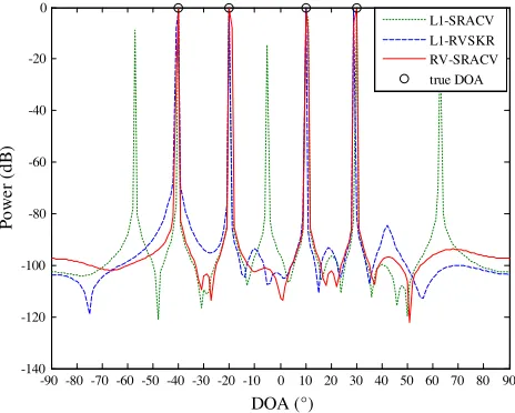
In the first simulation, the spatial spectra of the RV-SRACV algorithm is compared with L1-SRACV [9] and L1-RVSKR [11]. Consider four uncorrelated far-field narrowband signals arriving at the array from directions [−40◦, −20◦, 10◦, 30◦]. The grid is divided into 181 points in the range of −90◦ to 90◦ with 1◦ intervals. The number of snapshots is 300, and the signal-to-noise-ratio (SNR) is 0 dB. From Figure 1, it is observed that all algorithms succeed in estimating the four signals, but several pseudo-peaks appear with the L1-SRACV algorithm, and there is a slight bias in the spatial spectrum of the L1-RVSKR algorithm. On the other hand, the RV-SRACV algorithm has no pseudo-peak and shows better performance than L1-RVSKR, which means that the RV-SRACV algorithm’s robustness is enhanced.
-90 -80 -70 -60 -50 -40 -30 -20 -10 0 10 20 30 40 50 60 70 80 90 -140
-120 -100 -80 -60 -40 -20 0
DOA (°)
Po
w
e
r (
d
B
)
L1-SRACV L1-RVSKR RV-SRACV
true DOA
Figure 1. Spatial spectra for L1-SRACV, L1-RVSKR and RV-SRACV algorithm.
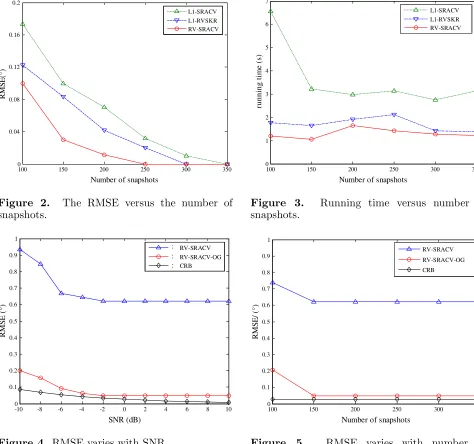
Then, the root-mean-square-error (RMSE) corresponding to the estimations in Figure 1 versus the number of snapshots is shown in Figure 2. The RMSE is defined as:
RMSE =
1
Q 1 K
Q
q=1 K
k=1
ˆ θkq−θk
2
(31)
where Q is the number of times of independent Monte Carlo experiments, and ˆθkq stands for the estimated angle of thekth signal in the qth Monte Carlo trial.
The SNR is 0 dB. The number of snapshots varies from 100 to 350 with 50 steps. For each number of snapshots,Q is 100. It can be seen from Figure 2 that the RMSEs of the three algorithms decrease with the increase of the number of snapshots. The RMSE of RV-SRACV algorithm is smaller than the other two algorithms under the same conditions. Conditions remain unchanged, and the running times of the three algorithms with different numbers of snapshots are shown in Figure 3. It can be seen from Figure 3 that the running time of RV-SRACV algorithm is the shortest, and it is illustrated in these simulations that RV-SRACV algorithm achieves better estimation performance with lower complexity. In the following simulation, RMSE of DOA estimation against SNR among SRACV, RV-SRACV-OG and Cramer-Rao Bound (CRB) is presented. The CRB of DOA estimation is given by [20]
CRB = σ 2
2
L
t=1
Re(XH(t)DHBDX(t)) −1
100 150 200 250 300 350 0
0.04 0.08 0.12 0.16 0.2
Number of snapshots
RM
S
E
(°
)
L1-SRACV L1-RVSKR RV-SRACV
Figure 2. The RMSE versus the number of snapshots.
100 150 200 250 300 350
0 1 2 3 4 5 6 7
Number of snapshots
runni
ng t
im
e
(s
)
L1-SRACV L1-RVSKR RV-SRACV
Figure 3. Running time versus number of snapshots.
-10 -8 -6 -4 -2 0 2 4 6 8 10
0 0.1 0.2 0.3 0.4 0.5 0.6 0.7 0.8 0.9 1
SNR (dB)
RM
S
E
(
°)
RV-SRACV RV-SRACV-OG CRB
: : :
Figure 4. RMSE varies with SNR.
100 150 200 250 300 350
0 0.1 0.2 0.3 0.4 0.5 0.6 0.7 0.8 0.9 1
Number of snapshots
R
M
S
E
/ (
°)
RV-SRACV
RV-SRACV-OG CRB
Figure 5. RMSE varies with number of snapshots.
whereX= diag{s1(t), . . . , sK(t)},B=I−A(AHA)−1AH,D= [∂θ∂A1, . . . ,∂θ∂Ak].
Consider a far-field narrowband signal that the true DOA is off-grid. It is selected randomly in independent Monte Carlo simulations, and Q = 100. We set g = 2◦ and ρ = 2.5. The number of snapshots is set to 300, and SNR varies from −10 dB to 10 dB with 2 dB steps. Figure 4 shows the comparison of the RMSE of DOA estimation versus SNR. From the simulation result, we know that the RMSE decreases with the increase of SNR and can be decreased by RV-SRACV-OG algorithm, and after that it is close to RMSE of the CRB.
signal-to-noise ratio and lower number of snapshots.
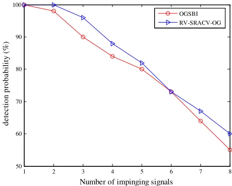
In the final simulation, the detection probability of DOA versus the number of impinging signals between RV-SRACV-OG and OGSBI [12] is presented. The SNR is 0 dB. The number of snapshots is 300, andQ= 100. We setg= 2◦ andρ= 2.5. The number of impinging signals varies from 1 to 8 with 1 step. The directions of impinging signals are off-grid and randomly chosen from −90◦ to 90◦. The detection probability is equal to the number of times that the average estimation error is less than 0.5 in 100 experiments, and we define the average estimation error as follows:
E = 1 K
K
k=1
θˆkq−θk (33)
where E denotes the average estimation error. From Figure 6, we see that detection probabilities of the two algorithms decrease with the increase of the number of impinging signals. The simulation illustrates that the detection probability of the proposed algorithm is superior to OGSBI.
1 2 3 4 5 6 7 8
50 60 70 80 90 100
Number of impinging signals
d
e
te
c
tio
n
p
ro
b
a
b
ility
(%
)
OGSBI RV-SRACV-OG
Figure 6. Detection probability versus the number of impinging signals.
5. CONCLUSION
In this paper, we propose a off-grid DOA estimation based on sparse representation and Rife algorithm called RV-SRACV-OG. The algorithm is divided into two parts. The first one is RV-SRACV algorithm based on real-valued sparse representation of array covariance vectors. It has better performance than L1-SRACV and L1-RVSKR algorithm, can decrease the computational burden and eliminate the false peaks by a unitary transformation and a block diagonal matrix, respectively. The second one is Rife algorithm. It can correct the DOA estimation when the true DOA is not on the discretized sampling grids. Finally, the simulation results show that the proposed algorithm is effective and performs better than OGSBI. The algorithm may be applied to practical applications in the near future.
REFERENCES
1. Schmidt, R. O., “Multiple emitter location and signal parameter estimation,” IEEE Transactions on Antennas and Propagation, Vol. 34, No. 3, 276–280, 1989.
2. Weiss, A. J. and G. Motti, “Direction finding using esprit with interpolated arrays,” IEEE Transactions on Signal Processing, Vol. 39, No. 6, 1473–1478, 1991.
4. Massa, A., P. Rocca, and G. Oliveri, “Compressive sensing in electromagnetics — A review,”IEEE Antennas and Propagation Magazine, Vol. 57, No. 1, 224–238, 2015.
5. Shaghaghi, M. and S. A. Vorobyov, “An improved L1-SVD algorithm based on noise subspace for DOA estimation,” Progress In Electromagnetics Research C, Vol. 29, No. 12, 109–122, 2012. 6. Carlin, M., P. Rocca, G. Oliveri, F. Viani, and A. Massa, “Directions-of-arrival estimation through
Bayesian compressive sensing strategies,” IEEE Transactions on Antennas and Propagation, Vol. 61, No. 7, 3828–3838, 2013.
7. Carlin, M., P. Rocca, G. Oliveri, and A. Massa, “Bayesian compressive sensing as applied to direction-of-arrival estimation in planar arrays,”Journal of Electrical and Computer Engineering, Vol. 2013, 1–12, 2013.
8. Rocca, P., A. M. Hannan, M. Salucci, and A. Massa, “Single-snapshot DOA estimation in array antennas with mutual coupling through a multi-scaling BCS strategy,” IEEE Transactions on Antennas and Propagation, Vol. 65, No. 6, 3203–3213, 2017.
9. Yin, J. H. and T. Q. Chen, “Direction-of-arrival estimation using a sparse representation of array covariance vectors,”IEEE Transactions on Signal Processing, Vol. 59, No. 9, 4489–4493, 2011. 10. He, Z. Q., Q. H. Liu, L. N. Jin, and S. Ouyang, “Low complexity method for DOA estimation
using array covariance matrix sparse representation,” Electronics Letters, Vol. 49, No. 3, 228–230, 2013.
11. Chen, T., H. X. Wu, and Z. K. Zhao, “The real-value sparse direction of arrival estimation based on the Khatri-Rao product,” IEEE Sensors Journal, Vol. 16, No. 5, 693–706, 2016.
12. Yang, Z., L. Xie, and C. Zhang, “Off-grid direction of arrival estimation using sparse Bayesian inference,”IEEE Transactions on Signal Processing, Vol. 61, No. 1, 38–43, 2011.
13. Luo, X. Y., X. C. Fei, L. Gan, and P. Wei, “Off-grid direction-of-arrival estimation using a sparse array covariance matrix,” Progress In Electromagnetics Research Letter, Vol. 54, 15–20, 2015. 14. Liang, Y., R. Ying, Z. Lu, and P. Liu, “Off-grid direction of arrival estimation based on joint spatial
sparsity for distributed sparse linear arrays,”IEEE Sensors Journal, Vol. 14, No. 11, 20981–22000, 2014.
15. Chen, T., H. X. Wu, L. M. Guo, and L. T. Liu, “A modified Rife algorithm for off gird DOA estimation based on sparse representations,”IEEE Sensors Journal, Vol. 15, No. 11, 29721–29733, 2015.
16. Song, J., Y. F. Liu, and Y. Liu, “An interpolation-based frequency estimator synthetic approach for sinusoid wave,”International Conference on Wireless Communications, Networking and Mobile Computing, 1–4, 2011.
17. Zhao, Y., L. Zhang, and Y. Gu, “Array covariance matrix-based sparse Bayesian learning for off-grid direction-of-arrival estimation,” Electronics Letters, Vol. 52, No. 5, 401–402, 2016.
18. He, Z. Q., Z. P. Shi, and L. Huang, “Covariance sparsity-aware DOA estimation for nonuniform noise,” Digital Signal Processing, Vol. 28, No. 1, 75–81, 2014.
19. Du, R. Y., F. L. Liu, and L. Peng, “W-L1-SRACV algorithm for Direction-Of-Arrival estimation,” Progress In Electromagnetics Research C, Vol. 38, 165–176, 2013.