Munich Personal RePEc Archive
The Emergence of A Parallel World: The
Misperception Problem for Bank Balance
Sheet Risk and Lending Behavior
Inoue, Hitoshi and Nakashima, Kiyotaka and Takahashi,
Koji
Sapporo Gakuin University, Konan University, Bank of Japan
26 July 2018
Online at
https://mpra.ub.uni-muenchen.de/91625/
The Emergence of a Parallel World: The Misperception
Prob-lem for Bank Balance Sheet Risk and Lending Behavior
∗Hitoshi Inoue †
Australian National University
Kiyotaka Nakashima ‡ Konan University
Koji Takahashi § Bank of Japan
January, 2019
Abstract. We examine the reason why two opposing views on distressed
banks’ lending behavior in Japan’s postbubble period have coexisted: one is stag-nant lending in a capital crunch and the other is forbearance lending to low-quality borrowers. To this end, we address the measurement problem for bank balance sheet risk. We identify the credit supply and allocation effects of bank capital in the bank loan equation specified at the loan level, thereby finding that the “parallel worlds”, or the two opposing views, emerge because the regulatory capital does not reflect the actual condition of increased risk on bank balance sheets, while the market value of capital does. By uncovering banks’ efforts to increase regulatory capital in Japan’s postbubble period, we show that banks with low market capitalization, and which had difficulty in building up adequate equity capital for their risk exposure, decreased the overall supply of credit. Parallel worlds can emerge whenever banks are allowed to overvalue assets at their discretion, as in Japan’ postbubble period.
JEL classification: G01, G21, G28.
Keywords: bank capital structure; capital crunch; forbearance lending; loan-level data; bank asset risk; bank risk taking.
∗The authors especially thank Takashi Hatakeda, You Suk Kim, Satoshi Koibuchi, Kenneth Kuttner,
Daisuke Miyakawa, Toshiaki Ogawa, Yoshiaki Ogura, Tatsuyoshi Okimoto, Arito Ono, Takeshi Osada, Michiru Sawada, Masahiko Shibamoto, Etsuro Shioji, Kenta Toyohuku, Nobuyoshi Yamori, Wako Watan-abe, and participants of the 2018 AJRC Seminar at the Australian National University, the 2018 Asian Meeting of the Econometric Society, the 2018 Annual Meeting of the Nippon Finance Association, the 2017 Autumn Meeting of the Japan Society for Monetary Economics, and the 2017 Kansai Monetary Eco-nomics Workshop for valuable comments and discussions. The authors acknowledge financial support from a Grant-in-Aid from the Ministry of Education, Science, Sports and Culture. The views expressed here are those of the authors and do not necessarily reflect the official views of the Bank of Japan.
†Correspondence to Hitoshi Inoue, Crawford School of Public Policy, Australian National University,
Building 132, Lennox Crossing, Acton, ACT, Zip 2601, Australia, e-mail: [email protected]
‡Faculty of Economics, Konan University, Okamoto 8-9-1, Higashinada, Kobe, Zip 658-8501, Japan,
e-mail: [email protected]
§Bank of Japan, 2-1-1, Hongokucho, Nihonbashi, Chuo-ku, Tokyo, Zip 103-0021, Japan, e-mail:
“Additional lending to low credit rating firms was a counterintuitive criti-cism, especially for business people involved in bank lending. Such forbearance lending was very rare. Bank loan officers, making every effort to reduce their lending, were bitterly resentful of forbearance lending. It was quite strange that two types of criticism of distressed Japanese banks’ lending behavior— stagnant lending and forbearance lending—coexisted in the post-bubble pe-riod.” Miyauchi (2015, p. 278)
1. Introduction Of the financial crises in developed economies, the one in Japan after the collapse of the bubble economy in the early 1990s was unprecedented in terms of the length and depth of the subsequent economic downturn.1
Debates about the reasons for Japan’s prolonged stagnation have been raised accordingly (e.g., Motonishi and Yoshikawa (1999), Hayashi and Prescott (2002), and Hoshi and Kashyap (2004)), and the lending behavior of banks with impaired capital has been one of the most plausible explanations, as the postbubble period witnessed the malfunction of the banking system.
When a substantial adverse shock hits the economy and many borrowers become insol-vent, banks should theoretically face impaired capital, irrespective of whether their bank capital is evaluated at regulatory or market values. The theoretical literature predicts two types of lending behaviors by such impaired banks: one is stagnant lending in a capital crunch, and the other is forbearance lending. In the former type of lending, impaired banks that are subject to capital constraints decrease credit to borrowers, irrespective of whether they are good or bad borrowers.2
In the latter type, however, the impaired banks conduct window-dressing to avoid the realization of capital losses, and thus allocate more credit to insolvent borrowers, while hoping that their situations will improve.3
These two prac-tices have different theoretical backgrounds, but they have often been accused of being the
1 See, e.g., Hoshi (2001) for a discussion of Japan’s bubble economy and its collapse in the early 1990s.
2 Bernanke and Lown (1991) defined a credit crunch as “a significant leftward shift in the supply curve
for loans, holding constant both the safe real interest rate and the quality of potential borrowers”, and related a credit crunch to a capital crunch, providing evidence on the US economic crisis in the early 1990s. The theoretical literature on capital crunches includes Holmstr¨om and Tirole (1997), Calomiris and Wilson (2004), and Diamond and Rajan (2011).
3 The theoretical literature about forbearance lending includes Diamond (2001), Caballero et al. (2008),
source of the prolonged stagnation experienced since the 1990s in Japan.4
The two opposing explanations of the lending practices of impaired banks share the premise that the impaired banks worried considerably about the further deterioration of their balance sheets, but these opposing views differ sharply in explaining impaired banks’ lending behavior: stagnant lending in a capital crunch involves the issue of overall credit undersupply to all borrowers, whereas forbearance lending involves the issue of credit alloca-tion to low-quality borrowers. The empirical literature, however, has surprisingly provided mixed evidence supporting the two opposing views on the lending behavior of distressed Japanese banks in the postbubble period, as in Peek and Rosengren (2005), Gan (2007), and Watanabe (2007). In this paper, we explore the reason why such parallel worlds of dis-tressed banks’ lending behavior emerged in empirical investigations, particularly focusing on the misperception problem for bank balance sheet (bank default) risk.
Models of banking under asymmetric information have emphasized the potential con-flict of interest between banks and depositors (see, e.g., Diamond (1984) and Calomiris and Wilson (2004)). This information problem faced by banks encourages them to offer short-term (demandable) low-risk debt, concentrating most balance sheet risk in their cap-ital and thus insulating depositors from this risk. Therefore, it is important to determine whether banks are well capitalized enough to absorb their balance sheet risk and stabilize the banking system. In the postbubble period in Japan, the misperception problem for bank balance sheet risk occurred simultaneously with the introduction of regulatory cap-ital standards, although they were introduced to prevent an overall undersupply of credit in a capital crunch or prevent excessive risk taking by impaired banks in forbearance lend-ing. Figure 1 shows the bank market capital ratio and regulatory capital surplus in the postbubble period in Japan. We observe that the regulatory capital ratio continued to increase during the 1990s, while the market value of bank capital continued to decrease. This indicates that Japanese banks window-dressed their regulatory capital ratio, although they faced substantive increases in their default risk as measured by their market value. Indeed, the correlation between the two capital measures is −0.83, and hence they imply
seemingly contradicting information on bank capital deficits. The postbubble period in
Japan saw a considerable divergence of regulatory capital from its market value; thus, this period provides a good natural experiment that allows us to investigate whether and how such a divergence between the bank regulatory and market capital measures affects our un-derstanding of prevailing patterns of the lending behavior of troubled banks. In particular, we address the problem of the coexistence of two opposing views of the lending behavior of distressed Japanese banks in terms of the misperception problem for bank balance sheet risk, thereby demonstrating that the use of regulatory capital as a measure of bank balance sheet risk would lead to erroneous assessments of bank lending behavior.
Our study of the misperception of bank balance sheet risk and lending behavior extends recent empirical studies. Haldane (2014) and Bulow and Klemperer (2015) pointed out that regulatory measures of bank capital do not have predictive power for bank failures. Indeed, Bears Sterns, Wachovia, Washington Mutual, Fannie Mae, and Freddie Mac were all viewed by regulators as being well capitalized immediately before their failures. Haldane and Madouros (2012) and Sarin and Summers (2016) attempted to measure bank risk using both regulatory measures (e.g., the Basel III Tier I ratio) and market measures (e.g., credit default swaps and price–earnings ratios), and found that the market capital ratio (the market value of equity relative to total assets) has the most explanatory power in predicting bank failure. In addition, the market capital ratio of US major banks has declined not only in the precrisis period, but also after the crisis (Sarin and Summers (2016)).5
These studies focused on the misperception problem for bank balance sheet risk. However, our study examines this issue by addressing the possibility that such a misperception problem would cause erroneous assessments of bank lending behavior and lead to the coexistence of the two opposing views about it, as in the late 1990s in Japan. Because the late 1990s in Japan was a pre-banking-crisis period as well as a postbubble period, our analysis of this period should provide rich insights into the arrival of the banking crisis.
In this paper, to investigate the coexistence problem, we use a loan-level matched dataset of Japanese banks and their listed borrowers in the postbubble period of the late
5 Adrian and Shin (2014) theoretically explained the reason for the distinction between a bank’s book
1990s, as in Peek and Rosengren (2005) and Gan (2007). This is partially because loan-level data enable us to overcome the identification problem in terms of the controllability of demand factors in specifying the bank loan equation, and partially because testing the forbearance lending by lowly capitalized banks to their low-quality borrowers requires the inclusion of a firm performance variable in the bank loan equation. Loan-level data are superior to bank- and firm-level panel data in terms of data structure for overcoming the omitted-variable problem because of the difficulty of controlling borrower-side factors in the bank loan equation (see Khwaja and Mian (2008) and Jim´enez et al. (2012; 2014)).
Our analytical focus is on the effect of changes in bank capital (regulatory capital or market capital) BCAPit on the “allocation” of bank credits ∆LOANjit among good and
bad borrowers as well as on the “supply” of credits to those borrowers. The novelty of our analysis is that we strictly define the credit supply and the allocation effect as the first and the second derivative effects in the bank loan equation specified at the loan level. More concretely, the credit supply effect of bank capital involves the first derivative
∂∆LOANjit/∂BCAPit in the bank loan equation, which is the focus of previous studies
that found the existence of a capital crunch, irrespective of whether they used loan-level (Gan (2007)) or bank-level data (Watanabe (2007)). The credit allocation effect, however, involves the coefficient of an interaction term between the bank capital ratio and a firm performance variableFIRMjt, or the second derivative∂2
∆LOANjit/∂FIRMjt∂BCAPit, which
Peek and Rosengren (2005) used to show that forbearance lending prevailed in Japan’s postbubble period using loan-level matched data.
A positive first derivative implies that a capital crunch, or stagnant lending by lowly capitalized banks, prevailed in the postbubble/precrisis period of the late 1990s. Conversely, if the first derivative is negative for low-quality borrowers and the second derivative is positive (where the firm performance variable is defined so that its value become larger as the firm’s performance improves), credit misallocation from lowly capitalized banks to low-quality borrowers occurred. We focus on the signs of the two derivatives, and especially whether and how the divergence of regulatory capital from its market value produces the two opposing views on distressed banks’ lending behavior.
pro-vides evidence supporting forbearance lending in which lowly capitalized banks did not increase or decrease credits, but the credits were allocated more to low-quality borrowers in the postbubble period, as demonstrated by Peek and Rosengren (2005); that is, regu-latory capital produces insignificant and significantly positive estimates for the first and second derivatives, respectively. This result is observed only in the bank group with a larger regulatory capital buffer, and accordingly, it is quite consistent with the hypothesis of Peek and Rosengren (2005) that Japanese banks engaged in the window-dressing and patching-up of regulatory capital or the bank capital ratio. Conversely, the use of the market value of bank capital provides evidence for the existence of a capital crunch, in which lowly market-capitalized banks decreased credit to all borrowers even if they were good borrowers, as demonstrated by Gan (2007) and Watanabe (2007); that is, market capital produces significantly positive and insignificant estimates for the first and second derivatives, respectively. In contrast to the result for the regulatory capital measure, this result for the market measure does not qualitatively differ among bank groups (with lower, medium, and higher market capital ratios), but does quantitatively differ in that equity capital constraints in lending are more pronounced for banks in the lower market capital group. The above findings are robust even if we control for the survivorship bias for bank– firm relationships, employ the same type of nonlinear specification as Peek and Rosengren (2005), and use banks’ lending exposure to real estate in the bubble period instead of the market capital measure, as in Gan (2007) and Watanabe (2007).
The above findings reveal the true lending behavior of Japanese banks in the postbubble (pre-banking-crisis) period of the late 1990s. By simultaneously controlling for the two bank capital measures and their interaction effects in the bank loan model, we find that the supply and allocation effects (the first and second derivative effects) of the regulatory capital ratio completely vanish, and that only the supply effect of the market capital ratio survives; that is, in reality, stagnant lending following a capital crunch occurred, and not forbearance lending. This result is robust as it is independent of the selection of firm performance variables.
structure, which is based on the standard corporate finance theory emphasizing “normal market forces”: creditors require banks to build their capital to secure an adequate charter value, or demand more equity protection from banks with more portfolio risk (see, e.g., Flannery and Rangan (2008) and Gropp and Heider (2010) for empirical studies on bank capital structure; see, e.g., Hackbarth et al. (2006), Valencia (2016), and Corbae et al. (2017) for theoretical studies). Through this capital structure regression, we find that the market capital ratio is determined by standard corporate finance variables, whereas the regulatory capital ratio is not. This result is robust, and is independent of the levels of the two capital measures, although the market capital ratio of banks with lower market capital levels—banks facing a more severe capital crunch—is less sensitive to two determinants: profitability and asset volatility. Such insensitivity implies that lowly market-capitalized banks have difficulty increasing their market capital ratio in accordance with their prof-itability and uncertainty through issuing equity. Our findings from the capital structure regression suggest that in explaining bank lending behavior in relation to the capital struc-ture, how the capital structure is determined is important. Without investigating it, we cannot identify the background mechanism through which the capital structure affects banks’ lending behavior.
face equity capital constraints in lending. In addition, this tendency of a capital crunch is more noticeable for banks with lower market values of capital.
Our paper is organized as follows. Section 2 reviews the previous literature on distressed banks’ lending behavior and financial status in Japan, and then discusses the measurement problem for bank balance sheet risk. Section 3 presents our empirical model and explains our dataset. Section 4 reports the results of our empirical analysis and then shows that the parallel worlds, or the two views of troubled banks’ lending behavior, will emerge depending on whether regulatory capital or market capital is used as the proxy for bank balance sheet risk. Section 5 examines the lending behavior of Japanese distressed banks by simultaneously controlling for the two capital measures and the interaction between them. In this section, we also explore the reason why parallel worlds emerge by investigating the determinants of the two capital measures. Section 6 explores a key driver of the capital crunch among the determinants of the bank capital structure, thereby providing an insight into the lending framework of troubled banks. Section 7 offers conclusions.
2. Bank Balance Sheet Risk and Lending Behavior In this section, we review the literature on distressed banks’ lending behavior and financial status in Japan, and then discuss the measurement problem for bank balance sheet risk in assessing those lending behaviors.
2.1. Literature on Lending by Troubled Japanese Banks Here, we briefly review previous research on the lending behavior of troubled Japanese banks, particularly focusing on what measures they used as a proxy of bank balance sheet risk or bank default risk. As discussed below, we focus on Peek and Rosengren (2005), Gan (2007), and Watanabe (2007), partially because they allow us to highlight the measurement problem for bank balance sheet risk in analyzing distressed banks’ lending behavior, and partially because, like ours, the former two studies both used loan-level matched data, although they gave two opposing views on distressed banks’ lending behavior in the postbubble (precrisis) period in Japan.
capital crunch, or a debt overhang, in the postbubble period in the 1990s.6
These recent studies include Gan (2007) and Watanabe (2007). These two studies used each bank’s lending exposure to the real estate industry in the real estate bubble of the late 1980s as a proxy of bank balance sheet risk in the postbubble period. Watanabe (2007) used bank-level panel data from 1995 to 2000 and utilized lending exposure to the real estate industry as the instrumental variable for the regulatory capital ratio, thus providing evidence that a capital crunch existed in the late 1990s.7
Like us, Gan (2007) used loan-level matched data from 1994 to 1998, and thus demonstrated that banks with greater real estate exposure in the late 1980s had larger reductions in lending to borrowers during the capital crunch of the late 1990s.
In contrast to the above studies supporting the existence of a capital crunch, Peek and Rosengren (2005) showed that banks’ window-dressing to avoid the realization of losses on their balance sheets provided additional credit to low-quality firms in the postbubble period. Like our study, theirs used loan-level matched data from 1994 to 1999, and they included the regulatory capital ratio as a proxy of bank balance sheet risk in their bank loan equations. In terms of the implementation of prudential policy, Giannettie and Simonov (2013) examined the effects of Japan’s three public capital injections in 1998, 1999, and 2003 on capital-injected banks’ lending behavior using loan-level data from 1998 to 2004. They demonstrated that if capital-injected banks were still undercapitalized, those banks were more likely to lend to low-quality borrowers, using the regulatory capital ratio as a proxy of bank balance sheet risk.8
6 See Bernanke and Lown (1991), Peek and Rosengren (1995; 2000), Berrospide and Edge (2010), and
Carlson et al. (2013) for empirical research on capital crunches in the United States.
7 Using a bank-level panel dataset, Ito and Sasaki (2002) estimated a bank loan equation in Japan
from 1990 to 1993, as did Woo (2003) from 1991 to 1997, Ogawa (2003, Chapter 2) from 1992 to 1999, Montgomery (2005) from 1982 to 1999, and Hosono (2006) from 1975 to 1999. They all found that a decrease in the regulatory capital ratio caused a decrease in bank loans in the 1990s by including the regulatory capital ratio in their bank loan equations. However, unlike Watanabe (2007) and Gan (2007), they did not use an instrumental variable for the regulatory capital ratio, such as lending exposure to the real estate industry in the late 1980s; hence, their empirical results appear to be less robust and dependent on the sample periods used.
8 Unlike these two studies, Sekine et al. (2003) used firm-level panel data from 1986 to 1999, while
As reviewed above, previous research has focused on Japan’s bank lending behavior mainly in the late 1990s, and has provided mixed evidence on the stagnant forbearance lending of distressed banks. In this paper, we hypothesize that the coexistence of two opposing views can be ascribed to the difference in the choice of proxy for bank balance sheet risk used to assess the lending behavior of troubled banks. The research suggesting the existence of a capital crunch uses banks’ lending exposure to the real estate industry during the real estate bubble of the late 1980s as a proxy of bank balance sheet risk in the postbubble period, as in Gan (2007) and Watanabe (2007), while those suggesting the existence of forbearance lending used the regulatory capital ratio, as in Peek and Rosengren (2005). One possible reason for such a measurement problem for bank balance sheet risk in Japan is rooted in banks’ behavior under the regulatory policy implemented after the introduction of the regulatory capital standards. In the next subsection, we review this problem in the context of Japan’s regulatory policy for banks.
2.2. Misperception Problem for Bank Balance Sheet Risk In the postbubble/pre-crisis period in Japan of the late 1990s, the measurement problem of bank balance sheet risk emerged following the introduction of regulatory capital standards, although these stan-dards were originally aimed at preventing stagnant lending in a capital crunch or excessive risk taking by impaired banks in forbearance lending (see also Nakashima and Takahashi (2018a) for details).
In 1988, bank regulators in major industrial countries agreed to standardize capital requirements internationally, through the so-called Basel Accord. Subsequent to this, all Japanese banks struggled to meet these capital standards in the 1990s. During this period in Japan, land and stock prices fell continuously. Consequently, many loans granted during the bubble period in the late 1980s became nonperforming. Accordingly, banks that were more impaired and had less capital issued additional subordinated debt to inflate their
bank capital. They were able to do so because, under the local Japanese rules governing capital requirements, subordinated debt can be counted as Tier II capital (see, e.g., Ito and Sasaki (2002) and Montgomery (2005)). Japanese banks also used deferred tax assets to compensate for capital losses arising from unrealized losses on their holding stocks. This is because the government allowed banks to include their deferred tax assets in Tier I capital in 1998. At their discretion, bank managers estimated subjectively the total amount of deferred tax assets (see Skinner (2008)).
In the 1990s, these regulatory forbearance policies caused Japanese banks to engage in “patching up” their regulatory (that is, book) capital ratios (see, e.g., Shrieves and Dahl (2003)). In the late 1990s, the attitude of the Japanese government and regulatory authorities toward Japanese banks started to change, and they allowed them to enter bankruptcy or receive a capital injection. In 1998 and 1999, the government of Japan decided to infuse a large amount of capital into poorly capitalized banks in order to increase their capital adequacy ratios. These large-scale public capital injections allowed almost all Japanese banks to meet their capital standards (see, e.g., Watanabe (2007), Nakashima (2016), and Guizani and Watanabe (2016) on the Japanese bank recapitalization programs). However, the amount of nonperforming loans in Japanese banks only started to decrease after the Financial Revitalization Program, or the so-called Takenaka Plan, was executed in 2002 (see Sakuragawa and Watanabe (2009) for details).
Figure 1 shows the bank market capital ratio (defined as the ratio of the market value of bank equity to the market value of total assets) and the regulatory capital surplus (defined as the difference between a bank’s reported capital adequacy ratio and its regulatory target ratio, i.e., 8% for international banks and 4% for domestic banks) in the postbubble period in Japan. As shown in this figure, the regulatory capital ratio continued to increase during the 1990s because of Japan’s regulatory forbearance policies, while the market capital ratio continued to decrease because equity market participants believed that Japanese banks window-dressed their regulatory capital by overvaluing their capital and undervaluing their nonperforming loans (see Hoshi and Kashyap (2004; 2010)). In fact, the correlation coefficient of the two variables is−0.83 at the aggregate level. This tendency for the market
information on banks’ risk profiles, is also clearly observed in Figure 2, where the two variables appear to be negatively correlated in the postbubble period.
To illustrate some individual cases, Figure 3 shows the market capital ratio and the regulatory capital surplus of Fukutoku Bank and the Long-Term Credit Bank (LTCB), which went bankrupt in May 1998 and October 1998, respectively. The market capital ratio of Fukutoku Bank continued to decrease during the postbubble period, while its regulatory capital surplus rose sharply before bankruptcy. The regulatory capital surplus of LTCB increased from the mid 1990s, partially because of the public capital injection in March 1998, while its market capital ratio continued to decrease until it went bankrupt. This negative correlation between the two capital measures is also observed in other banks that went bankrupt in the 1990s, including Hyogo Bank and the Nippon Credit Bank.
Such distinct differences in the information content of banks’ risk profiles are also ob-served in the relation between banks’ lending exposure to the real estate industry during the real estate bubble of 1989 and regulatory capital. The left panel of Figure 4 shows that regulatory capital has little or no correlation with bank lending exposure to the real estate industry, with a correlation coefficient of 0.06. As shown in the right panel of Figure 4 however, the market value of capital and bank lending exposure to the real estate in-dustry are negatively correlated with a correlation coefficient of −0.46, indicating that the
bank market capital ratio in the postbubble period reflects information on bank lending exposure to the real estate industry in the bubble period. Given that the decline in real estate prices in the 1990s caused a deterioration of bank balance sheets, the negative corre-lation indicates that the market value of bank capital is likely to capture the soundness of bank balance sheets more precisely (see Gan (2007)) and Watanabe (2007)). In Subsection 5.3, we will identify the determinants of the two capital measures in terms of standard corporate finance theory emphasizing market forces, thereby examining why and how the two measures contain different information on bank balance sheets and produce the two opposing views of troubled banks’ lending behavior.
ex-posure to the real estate industry) can capture bank default risk in the postbubble period in the 1990s, while regulatory capital cannot capture it because troubled Japanese banks were allowed to overvalue their portfolios at their partial discretion under the framework of the Basel Accords. As discussed in the Introduction, this insight is consistent with the findings of recent empirical studies on the misperception problem for bank balance sheet (or bank default) risk before and after the 2008 financial crisis (Haldane and Madouros (2012) and Sarin and Summers (2016)), which demonstrated that the market capital ratio had outstanding explanatory power in predicting bank failures before the crisis, but the regulatory capital ratio did not.
With due consideration of such a misperception problem for bank balance sheet risk, we have the legitimate expectation that any conclusion about the lending behavior of distressed banks depends heavily on which of the two measures is used as a proxy of bank balance sheet risk. In the following, we will untangle this misperception problem for bank balance sheet risk and lending behavior by analyzing the bank loan equation.
3. Empirical Specification and Data In this section, we start by introducing an empirical specification for bank lending to examine the measurement problem for bank balance sheet risk and bank lending behavior, and then discuss the estimation methods and our dataset.
3.1. Specification for Bank Loan Equations and Estimation Method As dis-cussed in the Introduction, we use a loan-level matched dataset of Japanese banks and their listed borrowers to identify the effect of bank capital on lending in Japan’s postbub-ble period, as in Peek and Rosengren (2005) and Gan (2007). The loan-level matched data allow us not only to control for borrower-side factors through time*firm fixed effects, but also to analyze the credit allocation effect through the (second derivative) effect of the inter-action between bank capital and firm performance variables. To exploit these advantages of the loan-level matched data, we specify the bank loan equation as follows:
∆LOANjit =a0+a1BCAPit−1+a2BCAPit−1∗ FIRM
j
where the dependent variable, ∆LOANjit, indicates the growth rate of the total amount of loans outstanding between bank iand domestic listed firm j at time t. vi denotes banki’s
time-invariant fixed effects to control for its time-invariant unobservables, whileujt denotes
firm j’s time-varying fixed effects, or year∗uj with time dummies (year), to control for
the borrowing firm’s total demand factors at each sample period t. εjit is the stochastic
disturbance term.
As for an observable explanatory variable,BCAPit denotes a financial variable for bank
ithat is supposed to capture the adequacy of bank capital and the increase in bank default risk: either bank i’s market capital ratio (MARCAPit) or its regulatory capital surplus
(REGCAPit).
9
FIRMjt is firm j’s performance variable. In this paper, instead of using conventional measures of profitability such as the return on assets and the working capital ratio, we use two equity-based measures of franchise values for a firm’s business performance in the future: Tobin’sq (FQjt) and the distance to default (FDDjt). The reason is that these equity-based measures better capture a firm’s current and future profitability than the conventional profitability measures based on its past profit.10
Considering that banks tend to place more importance on a borrower’s future performance when they evaluate default risk, the equity-based measures are more appropriate for examining their lending behavior. Tobin’s q is defined as the ratio of the market value of firm i (VA) to its book
value, where the market value of the borrowing firm is defined as the sum of the market value of its equity (VE) and the book value of its total liabilities (D).
11
The distance to default is defined as
FDD =
ln (VA/D) +
r−1
2σ
2
A
/σA,
9 As discussed in Subsection 2.2, the bank market capital ratio is defined as the market value of a bank’s
equity divided by the market value of its total assets, where the market value of a bank’s total assets is defined as the sum of the market value of its equity and the book value of its total liabilities. We calculate the market value of equity by multiplying the end-of-year stock price by the number of shares. The regulatory capital surplus is defined as the difference between a bank’s reported regulatory capital ratio and its regulatory target ratio (8% for international banks and 4% for domestic banks).
10 We do not use the distance to default as an equity-based measure of bank default risk. This is because
the usual assumption of log-normally distributed asset values in structural models of default risk is not appropriate for banks because of the special nature of their assets. See Nagel and Purnanandam (2018) for details.
11 We calculate the market value of firm equity by multiplying the end-of-year stock price by the number
wherer is the risk-free rate, and σA is the volatility of firm assets. The distance to default
can be interpreted as the expected standardized difference between the market value of the firm and the book value of its liabilities. If the difference is small (large), a firm is in danger of bankruptcy (healthy). A decrease (increase) in distance-to-default implies greater (lesser) credit risk. We define the volatility of firm assets σA as σA=σE ×VE/VA. To estimate the
volatility of equity (σE), we calculate the standard deviation of the market value of equity
for the final month of a firm’s fiscal year and express the estimated volatility as an annual rate.12
We use the yield on one-year Japanese government bonds as a proxy of the risk-free rate (r). In this paper, we focus mainly on the estimation results obtained using Tobin’s
q because it can easily classify borrowing firms as good or bad at the reference value of 100: if Tobin’sq is not less than 100, the borrowing firm is categorized as a good borrower; otherwise, it is classified as a bad one. The equation additionally includes lending exposure and borrowing exposure as relationship variables. The lending exposure is defined as loans from bank i to firm j divided by the total loans of bank i. The borrowing exposure is defined in the same manner, as loans from bankito firm j divided by the total borrowings of firm j.
Note that to control for borrower-side factors in our bank loan equation with ujt, we
employ the fixed-effects approach proposed by Khwaja and Mian (2008) and Jim´enez et al. (2012; 2014). The fixed-effects approach assumes that all potential borrower-side factors are embodied in time-varying firm unobservables, which are captured by time*firm fixed effects (ujt).13 This approach enables us not only to specify our lending equation in a more
parsimonious way, as expressed in equation (1), but also to identify the effect of bank capital
12 More specifically, we calculate the annualized estimated volatility of the market value of equity as
follows:
σE
E,jt=
1
D(t)−1
D(t)
d(t)=1
retj,d(t)−retj,t
2
×D(t),
whered(t) (d(t) = 1,· · ·, D(t)) indexes trading days in firmj’s fiscal yeart. retj,d(t)denotes the daily rate
of change in equity valuation, andretj,d(t) is the average rate of change in equity valuation during fiscal
yeart.
13 Hosono and Miyakawa (2014) and Nakashima (2016) employed this fixed-effects approach with Japanese
on lending more rigorously by controlling for demand factors in a more comprehensive way. In the following analyses, we use equation (1) as the benchmark model, where borrower-side factors are fully controlled with time*firm fixed effects.
By controlling for lender-side factors as well as borrower-side ones with the fixed-effects approach through time*bank fixed effects, one can focus on the interaction effects and examine the issue of credit allocation in a more robust way. More specifically, we introduce the following specification for bank loans:
∆LOANjit =a0+a2BCAPit−1∗FIRM
j
t−1+vit+ujt +εjit, (2)
where we control for all potential lender-side factors by utilizing time-varying unobservables
vit. We also examine the interaction effects, or the second derivative effects, on credit
allocation using this double fixed-effects approach (see Jim´enez et al. (2014) and Nakashima et al. (2018) for the double fixed-effects approach).14
Like our study, Peek and Rosengren (2005) and Gan (2007) used loan-level matched data, but their way of specifying the bank loan equation is different from ours. Peek and Rosengren (2005) transformed the growth data of bank loans into binary outcome data, and then employed a random-effects probit model. We use a linear rather than a nonlinear model of bank lending for two reasons. First, nonlinear models tend to produce biased estimates in panel datasets with many fixed effects, leading to an incidental parameters problem and inconsistent estimates. Second, nonlinear fixed-effects models generate biased estimates of interaction effects (see Ai and Norton (2003) for details). Nonetheless, we also employ their nonlinear specification, thereby attempting to conduct a robustness check for the estimation results based on our linear specification. However, like our approach, Gan (2007) specified a lending equation in a linear regression model but, unlike ours, did not control for banks’ unobservables, and controlled for firms’ unobservables through time-invariant fixed effects.
14 Jim´enez et al. (2014) and Nakashima et al. (2018) employed the double fixed-effects approach to
Note that Peek and Rosengren (2005) used regulatory capital surplus as a proxy for bank balance sheet risk and focused on the interaction terms between this bank financial variable and firm performance variables. However, instead of using the bank capital ratio, Gan (2007) used banks’ lending exposures to the real estate industry in 1989 in order to identify loan supply effects of banks’ impaired capital. In contrast to these two studies, Watanabe (2007) used a bank-level panel dataset and then used lending exposure to real estate as the instrumental variable of the regulatory capital ratio, thus providing evidence that a capital crunch existed in the late 1990s. In Section 4, we also apply these specifications to our data as a robustness test.
The advantage of our loan-level analysis based on equations (1) and (2) is that we identify the credit supply and the allocation effects as the first and second derivative effects, respectively. In these specifications, the first derivative, ∂∆LOANjit/∂BCAPit−1 = a1 +
a2FIRMjt−1, captures the effect of bank capital changes on credit supply, and the second
derivative, ∂2
∆LOANjit/∂FIRMjt∂CAPit = a2, measures the bank capital effect on credit
allocation among better- and worse-performing firms. If the first derivative has a positive value for all values of the firm performance variableFIRMjt−1, then a capital crunch prevails
in a period of bank distress. However, if the first derivative has a negative value for low-quality firms (e.g., with a lower Tobin’s q) and the second derivative has a positive value, forbearance lending by lowly capitalized banks to low-quality firms prevails. We examine whether and how the two bank capital measures produce the two opposing views on distressed banks’ lending behavior by focusing on the first and the second derivatives, or the credit supply and allocation effects of bank capital.
3.2. Correcting for Survivorship Bias Our matched lender–borrower sample is based on a continuation of the lending relationship. According to the literature on relationship banking, the continuation of a bank–firm relationship depends on both the bank’s and the firm’s characteristics (Ongena and Smith (2001) and Nakashima and Takahashi (2018b)). In other words, we must address the survivorship bias that may arise from nonrandom assortative matching between banks and firms.
regression of loan growth based on the estimation method discussed above. To the extent that credit supply/allocation is a two-step process in which a bank first decides whether to lend and then decides how much to lend, the selection model provides an insight into both decisions.
Our probit regression includes one-period lags of four banks’ characteristics such as the market leverage ratio, six firms’ characteristics such as the interest coverage ratio, and three relationship factors such as the duration of the relationship between lenderiand borrowing firm j. We estimate the probit regression for the continuation of bank–firm relationships and then estimate the second-stage regression of the bank lending equation with the inverse Mills ratio. To take into account the possibility that the coefficients of the variables in the probit model are time-varying, as pointed out by Nakashima and Takahashi (2018b), we conduct a rolling estimation of the probit model year by year. The details of the estimation results are shown in Appendix A.
3.3. Dataset The empirical analysis developed in this paper uses a loan-level dataset comprising matched samples of Japanese banks and their borrowing firms listed in Japan. We construct our loan-level data using the Corporate Borrowings from Financial Institu-tions Database compiled by Nikkei Digital Media Inc. This database annually reports short-(a maturity of one year or less) and long-term short-(a maturity of more than one year) loans from each financial institution for every listed company on any Japanese stock exchange.
for our sample period. We combined the Nikkei database with the financial statement data of Japanese banks and their listed borrowing firms, also compiled by Nikkei Digital Media Inc.15
Our chief difficulty in working with the loan-level data was sorting through various bank mergers and restructures in our data. We recorded the date of all bankruptcies and mergers that took place in the Japanese banking sector in our sample period. First, we should note that whenever a bank ceased to exist in our data because of a bankruptcy, firms ceased reporting that financial institution as a source of loans. If firms ceased reporting a bank as a lender and we could not find any information on a bankruptcy or a merger of the lending bank, we set the outstanding amount of loans from the bank equal to zero. However, if we found evidence of a bankruptcy or merger of a bank and a firm had outstanding loans from the restructured bank before that event, and from a surviving bank after that event, we calculated the growth rate of the loan from the restructured bank as if the restructured bank had made both of the loans.16
In order to calculate the loan growth rate of a restructured bank, we traced to it all banks that predated it. Thus, if banks A and B merged in yeartto form bank C, bank C’s loans in yeart−1 were set equal to the sum of the loans for banks
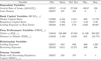
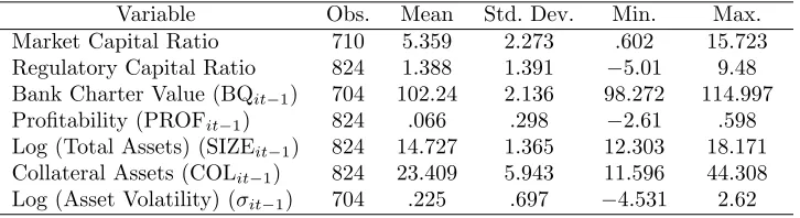
A and B, and the growth rate of bank C’s loans in year t would be calculated accordingly. Table 1 reports summary statistics for key variables, including the two bank capital variables and the firm performance variables of Tobin’sq and the distance to default.
4. Emergence of Parallel Worlds In this section, we report the estimation results for the two types of bank loan equations: that which uses the regulatory capital ratio and that which uses the market capital ratio. We show that the use of the two different capital measures produces the two opposing views, or parallel worlds, on lending by troubled banks: stagnant lending by banks with equity capital constraints and forbearance lending by banks
15 The end of the fiscal year for Japanese banks is March 31, but this is not necessarily the case for
borrowing firms. When combining the Nikkei database for loan-level data with the financial statement data of banks and their borrowing firms, we match bank-side information to borrower-side information in the same fiscal year.
16 As for exits of some firms from our loan-level dataset in the middle of our full-sample period, we cannot
identify reasons for firm exit from our sample, including bankruptcy, management buyout, termination of
all the firm’s relationships, etc. Therefore, if a firm exited from the original data after yeart, we dropped
the observation for the firm from our dataset in yeart. Thus, if the firm’s last observation in the original
engaging in patching-up of their regulatory capital.
4.1. Credit Supply and Allocation Effects We start by reporting the estimation results for the supply effect of bank capital on lending, or the first derivative effect, defined as ∂∆LOANjit/∂BCAPit−1 =a1+a2FIRMjt−1. Table 2 shows the estimation results for the
coefficient parametersa1 anda2, and Figure 5 shows the average supply effects for good and
bad borrowers where borrowing firms are classified into two groups as follows: if Tobin’s
q is not less than 100, the borrowing firm is labeled as a “good borrower”; otherwise, it is categorized as a “bad borrower”. As for the distance to default, a firm whose distance to default is higher than the sample mean is categorized as a good borrower; otherwise, it is classified as a bad one.
As shown in this figure, the use of the regulatory capital ratio yields a negative estimate for the average supply effect of a bad borrower with Tobin’sqequal to 50, although it is sta-tistically insignificant. We also find that the regulatory capital ratio produces significantly positive estimates for good borrowers with Tobin’s q values of 125 or more. These results indicate that the decrease in regulatory capital increases credit to low-quality borrowers, while decreasing credit to good borrowers during Japan’s postbubble period. When using the distance to default, we have insignificant estimates for firms facing higher default risk (whose distance to default is less than two), but significantly positive estimates for firms facing relatively lower credit risk (whose distance to default is greater than four).
The use of the market capital ratio however, produces significantly positive values for both good and bad borrowers. Furthermore, the result does not depend on whether Tobin’s
qor distance to default is used as the firm performance variable. This implies that a decrease in market capitalization would reduce credit to all borrowers irrespective of borrowers’ risk levels.
Table 2 also presents the estimation results for the credit allocation effect of bank capital, or the second derivative effect: ∂2
∆LOANjit/∂FIRMjt−1∂BCAPit−1 =a2. This table shows
the credit allocation effects for the double fixed-effects model (2) as well as the baseline model (1).
positive estimates. This indicates that banks with less regulatory capital allocate more credit to borrowers with a lower Tobin’s q or distance to default.
In contrast, the market capital ratio produces conflicting results; that is, the double fixed-effects model yields an insignificant estimate, while the baseline model yields a sig-nificantly negative one. This tendency does not change whether we use Tobin’s q or the distance to default as the firm performance variable. Given that the double fixed-effects model can control for both lender- and borrower-side factors more thoroughly, we should attach more importance to the insignificant estimate based on this model. Hence, we in-fer that the use of the market capital ratio provides evidence supporting the existence of a capital crunch, in which banks with reduced equity capital would reduce credit to all borrowers equally, irrespective of borrowers’ risk levels.
In addition, note that the inverse Mills ratio yields significantly negative estimates, implying that survivorship bias exists in such a way that we would obtain biased estimates for the parameter coefficients without including this ratio. We find that this result is quite robust to the use of alternative samples (see also Table 4).17
The above results are based on a linear specification, as expressed in equations (1) and (2). Table 3, panel (A) reports the estimation results obtained by employing the nonlinear specification of Peek and Rosengren (2005): the probit model with borrowing-firm random effects.18
We observe that even if we employ the nonlinear specification, our findings are robust: the use of regulatory capital provides evidence supporting forbearance lending, while the use of the market value of bank capital provides evidence for the existence of a capital crunch.
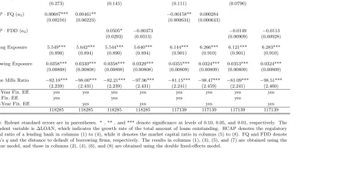
4.2. Lending Exposure to Real Estate in the Bubble Period As discussed in Sub-section 2.1, Gan (2007) and Watanabe (2007) assume that bank lending exposure to the real estate industry in Japan’s bubble period contains important information on Japanese banks’ balance sheet risk in the postbubble period. Table 3, panel (B) reports the estima-tion results obtained using bank lending exposure to real estate in 1989 instead of the two
17 Thus, we do not report the estimation results for the inverse Mills ratio except for Tables 2 and 4,
because of lack of space.
18 Note that Peek and Rosengren (2005) did not include lender-side unobservable covariates in their
bank capital measures.19
Note that the estimation results based on the lending exposure to the real estate industry are qualitatively the same as those obtained using the market capital ratio; that is, the model produces significant and insignificant estimates for the credit supply (first derivative) and allocation (second derivative) effects, respectively. This implies not only that banks with greater exposures to the real estate industry in the bubble period were more likely to decrease credit to all borrowers, but also that the market capital ratio contains similar information on Japanese banks’ lending behavior in the postbubble period to the banks’ exposure to the real estate industry in the bubble period in the late 1980s. Given that the high exposure of banks to the real estate industry is considered a cause of the deterioration of their balance sheets in the postbubble period that contributed to Japan’s banking crisis in the late 1990s, the market capital ratio appears to be a more appropriate indicator for capturing the relation between the condition of banks’ capital and their lending behavior.
4.3. Bank Lending with Low, Medium, and High Capital Ratios The capital crunch and forbearance lending views involve the issue of how much (or how little) bank capital is increased. To incorporate this issue into our analysis, we cluster our loan-level sample into three subsamples for banks with high, medium, and low capital ratios for each of the two capital ratio measures (i.e., market and regulatory). To construct the three subsamples, we define banks belonging to the first tertile (below the 34th percentile), the second tertile (34th–67th percentiles), and the third tertile (above the 67th percentile) of all banks as low, medium, and high capital banks, respectively. Table 4 shows the estimation results for the bank loan equations for banks with low, medium, and high capital based on the market and regulatory capital ratios.
In the upper panel (A), we find that the estimated coefficients for the market capital ratio are significantly positive for all three levels of the market capital ratio, but the esti-mated values (approximately two) for banks with a low level of market capital are much larger than those for banks with high and medium levels of market capital, each having almost the same value (approximately one). These results do not depend on the choice of
19 In the specification including lending exposure to real estate in the late 1980s, we do not include bank
the firm performance variable (Tobin’sq or distance to default).
The estimation results for the regulatory capital ratio in the lower panel (B) are sub-stantially different from those for the market capital ratio: the interaction effect, or the credit allocation effect, has significantly positive estimates for banks with a high regula-tory capital ratio. Furthermore, note that the results based on the subsample regression for banks with a high regulatory capital ratio more clearly demonstrate the forbearance lending by those banks, compared with the results based on the full-sample regression. In addition, the market capital ratio of those high capital banks is much lower than those of the two other bank groups in terms of the sample mean. These findings indicate that banks that were more engaged in window-dressing and patching-up their regulatory capital provided more credit to low-quality borrowers while those banks were facing low market values of equity capital.
4.4. Banks with Impaired Regulatory Capital The above positive estimates for the double interaction effect, or the credit allocation effect, based on the use of the regulatory capital ratio, may only reflect that banks with increasing regulatory capital provided more credit to high-quality borrowers; that is, the positive estimates could not identify forbear-ance lending to low-quality borrowers by impaired banks. To further address this identifi-cation issue, we also include a triple interaction term,BDECit−1∗REGCAPit−1∗FIRMjt−1,
in the bank loan equations (1) and (2). BDECit−1 is a dummy variable revealing the banks
that decreased their regulatory capital from yeart−2 tot−1. Approximately 35% of banks
in our sample were such capital-decreasing banks. If the triple interaction term has a posi-tive coefficient—or even if it is not posiposi-tive, as long as the inclusion of it does not eliminate the significantly positive effect of the double interaction term, REGCAPit−1 ∗FIRMjt−1—
then this implies that banks with decreased regulatory capital provided more credit to low-quality borrowers under forbearance lending.
effect of the double interaction term for banks with high regulatory capital. These results indicate that the positive estimates for the double interaction effect capture forbearance lending to low-quality borrowers by impaired banks.
4.5. Parallel Worlds of Japan’s Postbubble Period Summing up our estimation results for the postbubble period in the late 1990s, the use of the market capital ratio and bank lending exposure to the real estate industry in 1989 provides evidence supporting the existence of a capital crunch, in which banks with impaired capital decreased credit to firms irrespective of whether they were good or bad borrowers, as found by Gan (2007) and Watanabe (2007). The degree of capital constraints in bank lending was higher for banks with lower market capital; however, evidence of a capital crunch is widely observed, regardless of the value of the market capital ratio. However, the use of the regulatory capital ratio provides evidence supporting the existence of forbearance lending, in which impaired banks increased credit to low-quality borrowers, allocating more credit to those firms, as demonstrated by Peek and Rosengren (2005). In contrast to the case of market capital constraints, regulatory capital constraints in forbearance lending were observed only for banks with higher regulatory capital, which faced lower market capital ratios. Furthermore, the above findings for the market and the regulatory capital measures are observed in a robust manner when we control for the survivorship bias of bank–firm relationships, and do not depend on whether we adopt linear or nonlinear specifications. In the next section, we will explore the real world of lending by Japanese distressed banks while simultaneously controlling for the two capital measures and their interaction in the bank loan equation.
theory emphasizing market forces as its determinants. By doing so, we examine the reason why the parallel worlds of the two opposing views emerged.
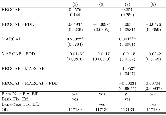
5.1. Controlling for the Two Bank Capital Ratio Measures Simultaneously In this subsection, we simultaneously control for the market and regulatory capital ratios and their interaction, thereby examining which of the two capital measures can explain bank lending behavior. As shown in Figure 1, and as pointed out by the recent empirical studies on bank balance sheet risk (Haldane and Madouros (2012), Haldane (2014), Bulow and Klemperer (2015), Sarin and Summers (2016), and Begley et al. (2017)), highly negative correlations between regulatory capital and the market value of equity capital are one piece of evidence of the misperception problem in measuring bank balance sheet risk based on the regulatory capital ratio. Taking into account that such negative correlations affect the estimation results for the bank loan equations and produce the two opposing views on troubled banks’ lending behavior, we control for the source of misperception: the interaction of the two capital measures. More concretely, we introduce the two interaction terms
REGCAPit∗MARCAPit and REGCAPit∗MARCAPit∗FIRMjt. The double interaction term
(REGCAPit∗MARCAPit) and the triple interaction term (REGCAPit∗MARCAPit∗FIRMjt)
are included to control for the interaction between the regulatory capital ratio and the market capital ratio, and for the allocation effect through the interaction of the two capital measures, respectively. By including the two interaction terms in the bank loan equation in order to investigate the source of misperception, we control for the interaction effect of the two capital measures and thus address distressed banks’ lending behavior in a more comprehensive way.
Table 6 shows the estimation results obtained by simultaneously controlling for the two capital measures and the two interaction terms in bank loan equations (1) and (2). As shown in columns (1), (2), (5), and (6) of panels (A) and (B), the simultaneous inclusion of the two capital measures yields significant coefficients for the two capital measures (REGCAP and
MARCAP), and for their two interaction terms with the firm variables (REGCAP∗FIRM
and MARCAP∗FIRM). However, the inclusion of the interaction terms between the two
capital measures (REGCAP∗MARCAP and REGCAP∗MARCAP∗FIRM) eliminates the
between the regulatory capital ratio and the firm variables, as shown in columns (3), (4), (7), and (8). These results indicate that stagnant lending in a capital crunch, but not forbearance lending to low-quality borrowers, prevailed overall in the Japanese banking system during the postbubble period.
Tables 7 and 8 report the results based on the subsample regressions for banks with high, medium, and low levels of market and regulatory capital. As with the full-sample regression in Table 6, the subsample regressions for banks with low, medium, and high market capital ratios in panel (A) also yielded significant coefficients for the two capital measures and their two interaction terms with the firm variables. However, again, controlling for the interaction between the two capital measures eliminates the significance of the regulatory capital ratio and the two interaction terms between it and the firm variables.
However, unlike the full-sample regression, the subsample regression for banks with high regulatory capital yields positive coefficients for the double interaction terms be-tween the regulatory capital ratio and the firm performance variable (REGCAP∗FQ and
REGCAP∗FDD), as shown in columns (21) to (24) of Tables 7 and 8. Furthermore, note
that the market capital ratio (MARCAP) for the banks with high regulatory capital has a significantly positive coefficient, but that for the banks with low and medium regula-tory capital does not, implying that only high regularegula-tory capital ratios have systematically negative correlations with the market capital ratio (see the sample mean of the regulatory capital ratio and the market capital ratio in panel (B) of Table 4). These results suggest that only banks with low market capital and high regulatory capital allocated more credit to low-quality borrowers, while decreasing credit overall in a capital crunch.
5.2. Banks with a Low Market Capital Ratio and High Regulatory Capital
Ratio To furtherer investigate the possibility that the forbearance lending view could still be accurate for banks with a low market capital ratio and high regulatory capital ratio, we estimate bank loan equations (1) and (2) using the sample of banks in the third tertile (above the 67th percentile) based on the market capital ratio and the first tertile (below the 34th percentile) for the regulatory capital ratio.
(MARCAP) is significant in all specifications, but not the interaction terms of the regula-tory capital ratio and the firm performance variable (REGCAP∗FQ and REGCAP∗FDD), as shown in panels (A) and (B) of Table 9.
Given that the market capital ratio remains significant, bank lending behavior in Japan’s postbubble period, or pre-banking-crisis period, of the late 1990s should be characterized as stagnant lending by banks subject to equity capital constraints in a capital crunch, instead of as forbearance lending.
5.3. Determinants of the Market and Regulatory Capital Ratios In the previ-ous subsection, we demonstrated that bank lending behavior in Japan’s postbubble period can be characterized as a capital crunch in which banks with equity capital constraints decreased credit to borrowers irrespective of borrowers’ risk levels. Here, we examine the reason why the two bank capital measures moved in opposite directions and the two oppos-ing views emerged. To this end, we analyze the determinants of the market and regulatory capital ratios, following the empirical analyses of Flannery and Rangan (2008) and Gropp and Heider (2010). These studies attempted to identify the determinants of bank capi-tal structures using cross-sectional regressions. Their econometric specification based on corporate finance theory are is follows:
BCAPit=α0+α1BQit−1+α2σit−1+α3PROFit−1+α4ln SIZEit−1+α5COLit−1+ǫit, (3)
where BCAPis the regulatory capital ratio or market capital ratio. The explanatory vari-ables are the bank’s Tobin’s q, or the bank charter value (BQ), the logarithmic value of the bank’s asset volatility, or the bank’s total risk exposure (σ), profitability (PROF), the logarithmic value of total assets (SIZE), and the value of collateral assets (COL). We in-clude the bank’s Tobin’s q and asset volatility, defined in the same manner as the firm’s Tobin’s q and asset volatility (see Subsection 3.1). We define the profitability as the return on assets in percentage terms, and the collateral assets as 100×(Liquid Assets +
Tangible Assets)/Total Assets.20
All variables are lagged by one year. The regression also
20 More concretely, we define Liquid Assets as Total Securities + Treasury Bills + Other Bills + Bonds +
includes time and bank fixed effects (year and ui) to control for unobserved heterogeneity
across time and among banks that may be correlated with the explanatory variables. Table 10 reports the summary statistics for those variables.
In Subsection 4.3, we found that the use of the market capital ratio as a measure of bank balance sheet risk leads to evidence that banks with a lower market capital ratio were more severely capital constrained in their lending than those with a medium or higher capital ratio, although all Japanese banks faced a capital crunch. However, we found that use of the regulatory capital ratio leads to evidence that only banks with higher regulatory capital engaged in forbearance lending. To incorporate these findings into our analysis of bank capital structure, we also estimate equation (3) by additionally including interaction terms between the five explanatory variables and the lower-market-capital dummy in the regression for the market capital ratio, and interaction terms between the five explanatory variables and the higher-regulatory-capital dummy in the regression for the regulatory capital ratio. Thus, we provide a detailed analysis of why there are two opposing views regarding troubled banks’ lending behavior.
The explanatory variables in equation (3) are conventional ones for explaining capital structure on the basis of standard corporate finance theory emphasizing market forces.21
According to this so-called market view, banks’ Tobin’s q is expected to have a positive coefficient because banks would protect a valuable charter by lowering their leverage and thus by lowering their default risk. Moreover, bank profit would also have a positive coefficient, as higher profits and sticky dividends allow banks to accumulate capital. Banks’ total risk exposure, defined as asset volatility, should also have a positive coefficient based on the inference that counterparties demanded more equity protection from banks with greater portfolio risk and business uncertainty. However, there is no clear prediction on how collateral and size affect capital building in terms of standard corporate finance theory. In contrast to the corporate finance view (or the market view), one alternative view places emphasis on the impact of capital regulation. It predicts that the standard corporate finance determinants have little or no explanatory power because market forces are not the
Heider (2010)).
21 Corporate finance theory regarding capital structure documents the role of dividends. However, we do
main driving force for banks to build up their capital. The other alternative is the “buffer” view, according to which banks tend to hold capital buffers above minimum regulatory requirement levels to avoid the costs that arise from issuing equity at short notice (see Gropp and Heider (2010) for the buffer view). This buffer view predicts that banks with higher profits and higher Tobin’sq are likely to be more leveraged because such banks face fewer asymmetric information problems, and their costs associated with issuing equity are relatively low.
Table 11 shows the results for the regressions for the market and regulatory capital ratios. In this table, we observe that the two capital ratios have quite different results, which well characterize the capital building behavior by Japanese banks in the late 1990s. More concretely, standard corporate finance variables significantly determine the market capital ratio, while none of them determines the regulatory capital ratio. This means that during the postbubble period, or the pre-banking-crisis period, in the late 1990s, banks’ equity capital reflected normal market forces, but their regulatory capital did not. In other words, in that period, neither the market view nor the buffer view is applicable to the regulatory capital ratio.
A significantly positive estimate for the Tobin’sq(BQ) indicates that the market capital ratio is associated with banks’ charter value, or future cash flows, while the regulatory capital ratio is not. Given that the sample mean of the regulatory capital ratio continued to increase, but that of the market capital ratio continued to decrease during the late 1990s, we infer that Japanese banks were not able to maintain their market capital to protect a valuable charter given the deteriorating Japanese economic conditions, while they were able to somehow increase regulatory capital, irrespective of the decreasing charter value.22
In other words, as the charter value decreases, banks tend to become more leveraged (see Calomiris and Nissim (2014) on United States banks).23
The positive coefficient for banks’ total risk exposure (σ) suggests that Japanese banks were substantially subject to market forces: counterparties demanded more equity protec-tion from banks with greater portfolio risk (see, e.g., Hackbarth et al. (2006), Flannery
22 In the late 1990s, low bank profits also contributed to the decrease in the market capital ratio.
23 Calomiris and Nissim (2014) examined declines in United States banks’ Tobin’s q after the financial
and Rangan (2008), Valencia (2016), and Corbae et al. (2017)). However, banks facing greater business uncertainty were not able to build up equity capital during the postbubble period. Indeed, as shown in Figure 5, the market capital ratio continued to decrease during Japan’s pre-banking-crisis period in the late 1990s, while banks’ asset volatility remained stable. By contrast, the insignificant estimate for the regulatory capital ratio implies that Japanese banks built up regulatory book capital without being exposed to market forces. The estimation results for Tobin’sq and risk exposure highlight the difference between the responses of the market and regulatory capital ratios to market forces.
However, even in the regression for the market capital ratio, Tobin’sq and banks’ total risk exposure have different estimates depending on whether a bank enters into the lower-market-capital group or not. More concretely, the interaction term of Tobin’s q and the lower-market-capital dummy does not have significant estimates, whereas that of banks’ risk exposure has significantly negative estimates, implying that the market capital ratio of the lower-market-capital banks reflects their portfolio risk less well. This is primarily because such banks were not able to issue equity and increase market capital, even if they faced greater portfolio risk or tried to take on more risk.
The estimation results for the other explanatory variables in the market capital equation are also quite consistent with corporate finance theory and previous research on bank capital structure (Flannery and Rangan (2008) and Gropp and Heider (2010)), but those in the regulatory capital equation are not. Also note that the insensitivity of regulatory capital to the conventional explanatory variables is observed in all Japanese banks—with lower, medium, and higher levels of regulatory capital.
difficulty in issuing equity, given the high volatility in their assets. Thus, their market capital is less sensitive to their total risk exposure and profits. Another explanation for the heterogeneity in the impacts of profits is that the “buffer” view starts to become effective as banks’ market capital ratios decrease: i.e., banks with less capital make efforts to find a way to increase their regulatory capital as a buffer against their profits decreasing, which weakens the positive association with bank market capital.
Bank size (SIZE) and collateral assets (COLL) have significantly positive coefficients for the regression with the market capital ratio, and the results do not depend on banks’ capital level because the interaction effects are not significant. The positive coefficient for bank size implies that larger banks hold more equity capital, but regulatory capital is accumulated irrespective of bank size. The positive coefficient for collateral assets (COLL) in the market capital equation implies that an increase in banks’ collateral assets induces them to increase their market capitalization. This is probably because such an increase in banks’ collateral assets is favored by market participants, and thus larger amounts of collateral may contribute to banks’ market capital.