Capital Accumulation and the Rate of Profit in a Two Class Economy with Optimization Behavior

Munich Personal RePEc Archive

Capital Accumulation and the Rate of

Profit in a Two-Class Economy with

Optimization Behavior

Sasaki, Hiroaki

7 August 2018

Online at

https://mpra.ub.uni-muenchen.de/88362/

Capital Accumulation and the Rate of Profit in a

Two-Class Economy with Optimization Behavior

Hiroaki Sasaki

August 2018

Abstract

By building a growth model with two classes, workers and capitalists, this study in-vestigates the existence and the stability of the long-run equilibrium along the lines of Pasinetti (1962) and Samuelson and Modigliani (1966). Unlike preceding studies in which the propensity to save of each class is exogenously given, this study assumes that workers solve a two-period overlapping generations model while capitalists solve an infinite-horizon dynamic optimization model. Depending on the combinations of both classes’ time preference rate, the parameter of the production function, and the popula-tion growth rate, we obtain two kinds of long-run equilibria, the Pasinetti equilibrium and dual equilibrium `a la Samuelson-Modigliani. We show that under realistic values of the parameters, the economy is likely to converge to the Pasinetti equilibrium.

Keywords: workers and capitalists; intertemporal optimization; Pasinetti equilibrium; dual equilibrium

JEL Classification: E13; E21; E25

1

Introduction

The purpose of this study is to theoretically investigate the existence, stability, and prop-erty of the steady-state equilibrium of the economy in which workers and capitalist coexist. Unlike previous studies that assume the constant propensities to save of both classes, we as-sume that both workers and capitalists solve dynamic optimization problems. This leads to revealing to the fundamental nature of the capitalist economy and contributes to the debate of income distribution policy in the long run.

∗

There exists much literature that investigates the property of the long-run equilibrium in a growing economy in which workers and capitalists coexist.

Pasinetti (1962) is a pioneering study and presents the “Pasinetti theorem” such that the long-run profit rate is given by the natural growth rate divided by capitalists’ propensity to save as long as the capitalists’ propensity to save exceeds the workers’ propensity to save. This theorem shows that the long-run profit rate is independent of the workers’ propensity to save.

On the contrary, Samuelson and Modigliani (1966) point out that the derivation of the Pasinetti theorem hinges on the implicit assumption that the capitalists’ propensity to save is considerably larger than the workers’ propensity to save. In addition, they show that unless the implicit assumption is satisfied, the long-run profit rate is given by the natural growth rate times the output elasticity of capital divided by the workers’ propensity to save. This is called the “dual theorem”.

After these two studies, many researches are produced that modify the specifications and assumptions of models and examine whether the Pasinetti theorem and the dual theorem are theoretically and empirically valid.

However, almost all previous studies assume that both the workers’ propensity to save and capitalists’ propensity to save are constant through time: both classes are agents that do not make future consumption plans.

In contrast, this study assumes that workers and capitalists are rational agents that make future consumption plans given the life-time budget constraints. Specifically, workers solve a two-period over-lapping generations problem while capitalists solve a infinite-horizon Ramsey problem.1

Such an attempt is also done by Michl and Foley (2004). They build a growth model in which workers solve a two-period overlapping generations model and capitalists solve an infinite-horizon dynamic optimization model. They use a fixed coefficient Leontief pro-duction function and let the real wage rate exogenously given according to the Classical assumption. However, in reality, substitution between labor and capital are observed in the long run. Moreover, many developed countries experience near-full employment in the long run, and hence, the real wage rate is adjusted to equate labor demand and labor supply.

For this reason, thus study uses a neoclassical production function with labor-capital substitution and assumes that the real wage rate is endogenously determined by the full employment condition. Using the model, we investigate (1) whether the long-run

equilib-1_{The importance that macroeconomists should consider agents with different saving propensities is}

rium exists, (2) how many equilibria exist if they exist, (3) whether the long-run equilibrium is stable, (4) to which equilibrium the economy converges, and (5) how fast the speed of convergence is.

The contribution of this study is as follows.

Many existing studies including Pasinetti (1962) use two state variables, workers’ own capital stock and capitalists’ own capital stock. Accordingly, those systems are a system of two-dimensional first-order differential equation or a system of two-dimensional first-order difference equation. Therefore, it is difficult to examine the speed of convergence toward the long-run equilibrium from initial values. In contrast, from our model, we can derive a one-dimensional second-order difference equation as well as a system two-dimensional first-order difference equation. For this reason, we can relatively easily compute the speed of convergence, and carry out numerical simulations.

Unlike the existing models that assume exogenously given propensities to save, the model of this study considers each class’s utility maximization. Accordingly, by using meaningful parameters that specify the shape of the utility function, and not by arbitrary parameters—saving rate, we can obtain conditions under which the Pasinetti equilibrium and the dual equilibrium occur. For example, if the government conducts a policy of income redistribution, workers and capitalists are expected to change their saving rates in response to the policy. However, models of constant saving rates cannot consider this change in the saving rates. On the other hand, since our model considers agents’ optimization behavior, the saving rate changes in response to economic policy. Therefore, we can strictly cap-ture the effect of economic policy. This property of the model are useful when conducting numerical simulations.

For related studies, we can refer to the following studies.

Kaldor (1956) presents an economic growth model in which the saving rate of workers and that of capitalists are different. However, as Pasinetti (1962) points out, Kaldor’s model is a model in which the propensity to save from wage and the propensity to save from profit are different.2

Pasinetti (1962) argues that if workers save, then workers obtain interest income by hold-ing capital stock through savhold-ing. Accordhold-ingly, the total capital stock of the whole economy is composed of workers’ own capital stock and capitalists’ own capital stock. In addition, he reveals that at the long-run equilibrium where workers and capitalists coexist, the profit rate is given by the natural growth rate divided by capitalists’ saving rate, which is called

2_{B¨ohm and Kaas (2000) build a discrete time growth model with a Kaldorian saving function and show the}

the Pasinetti theorem.

In contrast, Samuelson and Modigliani (1966) reveal that the derivation of the Pasinetti theorem critically hinges on the assumption that the capitalists’ propensity to save is much higher than the workers’ propensity to save. Then, they show that unless the assumption is satisfied, the dual equilibrium is obtained.

With regard to the debate between Pasinetti (1962) and Samuelson and Modigliani (1966), Furuno (1970) examines the speed of convergence toward the Pasinetti equilibrium and the dual equilibrium by building a neoclassical growth model with the Cobb-Douglas produc-tion funcproduc-tion.

Faria and Teixeira (1999) introduce a government sector into a two-class neo-classical growth model with the Cobb-Douglas production function. They show that for the steady-state equilibrium to be stable, the output elasticity of capital in the production function must be close to unity. In this case, the ratio of capitalists’ own capita stock to the total capital stock approaches unity, which is called the “anti-dual” equilibrium.3

Zamparelli (2017) also investigates the anti-dual equilibrium. He focuses on the case where the production function takes the constant-elasticity-substitution form, the elasticity of substitution exceeds unity, and endogenous growth occurs. In this case, the economy converges to the anti-dual equilibrium, capitalists’ own capital stock share approaches unity, and the profit share approaches unity.

Closest to our study is Commendatore and Palmisani (2009). They extend a model of Michl and Foley (2004) and present a model in which the real wage rate is endogenously determined by the full employment condition.4 _{In contrast to our study, they use a CES}

production function and investigate a case in which the elasticity of substitution between labor and capital is less than unity. In this case, chaotic dynamics occur depending on conditions. On the other hand, the present study uses a Cobb-Douglas production function. Interests of analysis are different from the present study. They focuses on the analysis of chaotic dynamics while we focus on the property of the steady-state equilibrium, the speed of convergence, and the dynamics of income distribution.

The remainder of this paper is organized as follows. Section 2 presents our model.

3

For the anti-dual equilibrium, see Darity (1981). He shows that using a effective demand constrained Keynesian model, there occurs the anti-dual equilibrium in addition to the Pasinetti equilibrium and the dual equilibrium. For studies that consider two different saving rates in demand-constrained Keynesian model, see Torii (2012) and Kumar, Schoder, and Radpour (2018). Van der Ploeg (1984) extends a Goodwin model to consider workers’ saving and shows that the dual equilibrium is stable while the Pasinetti equilibrium is unstable.

4_{For a two-class growth model with dynamic optimization, see Faria and Araujo (2004). They present}

Section 3 obtains the long-run equilibria, that is, the Pasinetti equilibrium and the dual equi-librium, and investigates the stability of each long-run equilibrium. Section 4 investigates to which equilibrium the economy converges by using parameter values obtained from eco-nomic data. Section 5 discusses the dynamic efficiency of the Pasinetti equilibrium and the dual equilibrium. Section analyzes the income distribution between workers and capitalists. Section 7 investigates the speed of convergence toward each long-run equilibrium. Section 8 concludes.

2

Model

Suppose an economy in which workers and capitalists coexist. Capitalists lend their own capital to firms, obtain interest income, and allocate interest income between consumption and saving. Capitalists behave as a dynasty that continues infinitely. Therefore, capitalists solve the infinite horizon dynamic optimization problem. In contrast, workers at the young period supply inelastically one unit of labor to firms and allocate the wage income between consumption and saving. At the old period, workers use their own saving to consume. Workers do not have bequest motive. Therefore, workers’ optimization problem is described as an over-lapping generations model.

2.1

Capitalists’ problem

Capitalists solve the following infinite horizon dynamic optimization problem:

max (1−_βc)

∞

∑

t=0

βt_clogC_tc, 0< βc <1,

s.t.Cc_t +K_tc+1 ≤ (1+rt)Ktc,

K₀c, rt : given,

whereβc denotes the discount factor of capitalist;Cc, consumption of capitalists; Kc,

capi-talists’ own capital stock; andr, the profit rate.

From the first-order necessary conditions, we obtain the Euler equation of consumption as follows:

From this, we obtain the following consumption function:

C_tc =(1−_βc)(1+rt)Ktc. (2)

The equation for capitalists’ capital accumulation is given by

K_tc₊₁ =βc(1+rt)Ktc. (3)

This equation shows that the capitalists’ propensity to save from stock wealth is given byβc.

Letsc denote the capitalists’ propensity to save from flow profit. Then,scis given by

sc =

rKc_−Cc

rKc = 1−(1−βc)

1+r

r . (4)

Along the transitional dynamics toward the steady-state equilibrium,rchanges, and hence, the capitalists’ propensity to save also changes. However, whenris constant at the steady-state equilibrium, the capitalists’ propensity to save is also constant.

2.2

Workers’ problem

Suppose that the number of workers is Lt, workers are fully employed, and Lt grows at a

constant raten. Workers solve the following two-period optimization problem.

max (1−_{βw) logc}w

1,t+βwlogcw2,t+1, 0< βw <1,

s.t.cw_1,t+ c

w

2,t+1

1+rt+1

≤ _wt,

wt, rt+1 : given,

where βw denotes the discount factor of workers; cw₁, workers’ consumption at the young

period;cw

2, workers’ consumption at the old period; andw, the real wage rate.

From this, we obtain the following consumption and saving functions.

cw_1,t =(1−β_w)wt, ₍₅₎

sw_t =βwwt, (6)

The equation for workers’ capital accumulation is given by

K_tw₊₁ = sw_t Lt =βwwtLt. (7)

2.3

Firms

Firms produce a good available for consumption and investment by using labor and capital inputs. Suppose that the production function is a constant-returns-to-scale Cobb Douglas production function, which is given byYt = KtαL1

−α

t , 0 < α <1. From profit maximization,

the real wage rate and the rate of profit are respectively given by as follows.

wt = w(kt)=(1−α)ktα, (8)

rt = r(kt)= αkα

−1

t , (9)

wherek = K/Ldenotes the capital stock per labor. We assume that capital stock does not depreciate.

3

Two-variable system

We investigate the dynamics of capital stock. Letkc _{= K}c_/Landkw _{= K}w_{/Lbe the}

capital-ists’ own capital stock divided by labor and the workers’ own capital stock divided by labor, respectively. Here, sinceK= Kc_+Kw_{, we havek= k}c_+kw_{. From equations (3) and (7), the}

dynamical equations ofkc

t andkwt are respectively given by

k_tc₊₁ = βc

1+n[1+r(kt)]k

c

t, (10)

k_tw₊₁ = βw

1+nw(kt), (11)

r(kt)= f

′

(kt), (12)

w(kt)= f(kt)−ktf′(kt), (13)

kt = ktc+k w

t . (14)

The steady-state equilibrium is a situation wherekc_t = k_tc₊₁ = kc, k_tw = k_tw₊₁ = kw. From equations (10) and (11), the steady-state values ofkcandkwsatisfy the following equations.

kc = βc

1+n[1+r(k)]k

c_{, (15)}

kw = βw

We investigate two cases: kc > 0 (interior solutions) andkc = 0 (corner solutions). Clearly,

kc _{= 0 satisfies equation (15). Substituting k = k}w _{= 0 into equation (16), we obtain}

w(0)= f(0)=0. Therefore, we obtain trivial solutionsk= kc _=kw_{= 0.}

3.1

Pasinetti equilibrium

Whenkc _{, 0, by dividing equation (15) byk}c_{, we obtain the steady-state equilibrium value}

ofk. Then, the profit rate does not at all depend on the shape of the production function and the marginal productivity of capital. Substitutingkinto equation (16), we obtain kw_{. From}

kc _=k−kw_{, we obtaink}c_{. This equilibrium is called the Pasinetti equilibrium since Pasinetti}

(1962) considers this case. When the production function takes the Cobb-Douglas form, the Pasinetti equilibrium is given by

kP =

(

1+n−_βc

αβc

)_α1−1

, (17)

kw_P = βw(1−α)

1+n

(

1+n−_βc

αβc

)α−11

, (18)

kc_P = kP−kwP, (19)

rP =

1+n−_βc

βc

, (20)

sc =

nβc

1+n−_βc. (21)

3.2

Dual equilibrium

Whenkc = 0, we have k = kw. From equation (16), we obtain kw and k. At this steady-state equilibrium, capitalists do not own capital stock. This equilibrium is called the “dual equilibrium” since Samuelson and Modigliani (1966) point out to criticize Pasinetti (1962). When the production function takes the Cobb-Douglas form, the dual equilibrium is given by

kD =kwD =

[

1+n βw(1−α)

]α1−1

, (22)

kc_D =0, (23)

rD =

α

1−_α

· 1+n

βw

4

Stability of long-run equilibrium

We investigate the stability of the Pasinetti equilibrium and the dual equilibrium by using phase diagrams.

Fromkc t+1 = k

c

t, we obtain

kc_t = −_kw

t +

(

αβc

1+n−_βc

)₁−1α

= −_kw

t +A. (25)

This is a straight line with the slope being−_{1 and the intercept being A>0.}

Fromkw t+1 = k

w

t , we obtain

kc_t = −_kw_t +

[

1+n

(1−_α)βw ·_kw_t

]1α

. (26)

Differentiating both sides with respect tokw

t , we have

∂kc t

∂kw t

=−₁+ 1

α

[

1+n

(1−_α)βw

]α1

(kw_t )1−αα. (27)

Whenkw

t =0, the sigh of the derivative is−1. Askwt becomes larger, the sign of the derivative

will become positive.

Moreover, substitutingkc

t =0 into equation (26), we obtain

kw_t =

[

(1−_α)βw

1+n

]₁−1α

= B. (28)

According to the sizes ofAandB, we obtain two-kinds of phase diagrams. The condition thatA> Bis given by

βw<

αβc(1+n)

(1−_α)(1+n−_βc). (29)

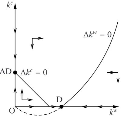
When A > B, we obtain a phase diagram given by Figure 1. In this case, we obtain two equilibria. Point P denotes the Pasinetti equilibrium and Point D denotes the dual equilib-rium. From Figure 1, we know that the Pasinetti equilibrium is globally stable while the dual equilibrium is globally unstable.

WhenA < B, we obtain a phase diagram given by Figure 4. In this case, we obtain an equilibrium. From Figure 4, we know that the dual equilibrium is globally stable.

k

k w O

AD

P

D k

=0

k w

=0

Figure 1: Convergence to Pasinetti equilibrium

k

k w O

AD

D k

= 0

k w

=0

Proposition 1. Suppose that βw < αβc(1+n)/[(1−α)(1+ n−βc)]. Then, there exist the

Pasinetti equilibrium and the dual equilibrium. The Pasinetti equilibrium is globally stable while the dual equilibrium is globally unstable.

Proposition 2. Suppose thatβw > αβc(1+n)/[(1−α)(1+n−βc)]. Then, there exists the

dual equilibrium. The dual equilibrium is globally stable.

From the above two propositions, we know that the economy converges to the Pasinetti equilibrium when βw < αβc(1 + n)/[(1− α)(1 + n − βc)] while it converges to the dual

equilibrium whenβw > αβc(1+n)/[(1−α)(1+n−βc)].

Theoretically, it is possible that the economy converges to each equilibrium. Then, we investigate whether the economy is likely to converge to the Pasinetti equilibrium or the dual equilibrium by giving numerical values to the parameters.

First, by considering the average capital share in developed countries, we set the capital share asα=0.3.

Second, according to de la Croix and Michel (2002), we use βw = 0.23. Since they

use the utility function such that u = logcw

1,t +βc w

2,t+1 and the value of β = 0.3, we use βw = β/(1+β) = 0.23 in our model. The reason why they useβ = 0.3 is that they set the

quarter discount rate as 0.99 and assume that the one period in the OLG model is 30 years:

β=0.994×30 _≈0.3.

Third, we usen = (1+0.01)30 _{−1 = 0.35 because we assume that annual population}

growth rate is 1%.

Fourth, according to Storm and Naastepad (2012), the average propensity to save from profit income in developed countries is 0.5. From the capitalists’ propensity to save at the Pasinetti equilibriumsc =nβc/(1+n−βc), we obtainβc =0.66.

From the above parameter values, we computeαβc(1+n)/[(1−α)(1+n−βc)] = 0.55,

wich is larger thanβw = 0.23. Then, the economy converges to the Pasinetti equilibrium.

Therefore, the economy in reality is likely to converge to the Pasinetti equilibrium.

5

Dynamic e

_ffi

ciency

We investigate whether the Pasinetti equilibrium and/or dual equilibrium is excessive sav-ing, that is, whether the equilibrium satisfies the dynamic efficiency. At the steady-state equilibrium, the capital stock per labor that maximizes consumption per labor is given by

kGR =

(α

n

)1−1α

We compare this value withkPandkD.

At the Pasinetti equilibrium, we obtain

sgn(kP−kGR)=−

α(1+n)(1−_βc)

n(1+n−_βc) <0, (31)

which suggests thatkP < kGR. Therefore, at the Pasinetti equilibrium, the dynamic ineffi

-ciency does not occur.

At the dual equilibrium, we obtain

sgn(kD−kGR)=

βwn(1−α)−α(1+n)

n(1+n) . (32)

This sign will be positive provided that

βw >

α

1−_α

· 1+n

n . (33)

This condition can be satisfied ifαis small and nis large. Then, we obtainkD > kGR, and

therefore, the dynamic inefficiency will occur.

Proposition 3. The Pasinetti equilibrium satisfies the dynamic efficiency while the dual equi-librium can be dynamically inefficient.

At the steady-state equilibrium of the typical Ramsey model, the modified golden rule is attained, and hence, excessive accumulation of capital does not occur. At the Pasinetti equi-librium of our model too, excessive accumulation of capital does not occur. In contrast, at the dual equilibrium, excessive accumulation of capital will occur depending on conditions, which is the same as the steady-state equilibrium of the typical OLG model such that only workers exist.

The relationship between the profit rate and the economic growth rate is as follows. We haver= nat the golden equilibrium,r> nat the Pasinetti equilibrium, andr⋛nat the dual equilibrium.

6

Income distribution between workers and capitalists

We examine income distribution between workers and capitalists. Using the Cobb-Douglas production function, the labor share and the capital share are 1−_{αandα, respectively. In}

Letσw andσc denote the workers’ income share and capitalists’ income share,

respec-tively. Then, we obtain

σw=

wL+rKw

Y =(1−α)+α kw

kw_+kc, (34)

σc =

rKc

Y =1−σw =α kc

kw_+kc. (35)

At the Pasinetti equilibrium, each class’s income share is given by

σw=

(1−_α)(1+n+βwα)

1+n , (36)

σc =

α[1+n−_βw(1−_α)]

1+n . (37)

Interestingly, these income shares do not depend on the capitalists’ discount factorβc. Each

class’s income share depends on the workers’ discount factor, the population growth rate, and the parameter of the production function.

At the dual equilibrium, each class’s income share is given by

σw =1, (38)

σc =0. (39)

Moreover, along the transitional dynamics toward the steady-state equilibrium, each class’s income share continues to change. Rewriting the workers’ income share as

σw =(1−α)+

α

1+ kct

kw t

, (40)

we see thatσwdecreases whenkct/kwt increases whileσwincreases whenkct/kwt decreases.

7

Speed of convergence to long-run equilibrium

We note that our model is also described as the second-order difference equation of one state variable K. Since the total capital stock of the economy is the sum of the capitalists’ own capital stock and the workers’ own capital stock, the capital stock att+1 is given by

Kt+1 = Kc_t+1+K

w

t+1. The workers’ own capital capita stock att+1 is given by K

w t+1 = s

w t Lt,

and hence, we obtain the following equation.

SubstitutingKc

t = Kt−Ktwinto the above equation, we obtain

Kt+1= βc(1+rt)(Kt−βwwt−1Lt−1)+βwwtLt. (42)

Dividing both sides with respect toLt+1, we have

kt+1 = βw

1+nwt+ βc

1+n(1+rt)kt−

βwβc(1+rt)wt−1

(1+n)2 . (43)

Substitutingrt =r(kt),wt = w(kt), andwt−1 =w(kt−1) into the above equation, we obtain the

second-order non-linear difference equation ofk.

When the production function takes the Cobb-Douglas form, the dynamical equation for capital accumulation is given by

kt+2 = βw

1+n(1−α)k

α

t+1+ βc

1+n(kt+1+αk

α

t+1)− βwβc

(1+n)2(1−α)(1+αk

α−1

t+1)k

α

t. (44)

Using this difference equation, we examine the speed of convergence toward the steady-state equilibrium.

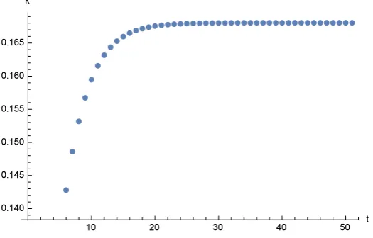
As mentioned above, Furuno (1970) computes the speed of convergence toward the Pasinetti equilibrium and the dual equilibrium. He reveals that it takes very long time for the economy converge to each equilibrium. For example, 90% convergence toward the dual equilibrium takes 500 years.5

Figure 3: Convergence speed to Pasinetti equilibrium

5_{Using the neoclassical growth theory, Sato (1963) computes the speed of convergence and shows that 90%}

Under our parameter setting, it takes about 40 periods to converge toward the Pasinetti equilibrium, which is shown in Figure 3. If the one period is 30 years, then the convergence toward the Pasinetti equilibrium takes 1200 years.6

8

Concluding remarks

This study builds a model in which both workers and capitalists conduct dynamic optimiza-tion and investigates the property and the stability of the long-run equilibrium. The intro-duction of dynamic optimizing behavior is largely different form previous studies including Pasinetti (1962) and Samuelson and Modigliani (1966).

Our results show that the economy can converge to the Pasinetti equilibrium or the dual equilibrium depending on the sizes of the parameters. The results also show that the econ-omy is likely to converge to the Pasinetti equilibrium under realistic values of the parame-ters. Samuelson and Modigliani (1966) and Furuno (1970) show that whether the economy converges to the Pasinetti equilibrium or the dual equilibrium depends on the three vari-ables: workers’ propensity to save, capitalists’ propensity to save, and capital share. In contrast, in our model, whether the economy converges to the Pasinetti equilibrium or the dual equilibrium depends on the four variables: workers’ time preference rate, capitalists’ time preference rate, capital share, and the population growth rate.

For income distribution, we can say that at the Pasinetti equilibrium, workers’ and cap-italists’ income shares do not depend on capcap-italists’ time preference rate. This result is contrasted to the result that the profit rate at the Pasinetti equilibrium does not depend on workers’ time preference rate.

References

B¨ohm, V., and L. Kaas (2000) “Differential Savings, Factor Shares, and Endogenous Growth Cycles”Journal of Economic Dynamics&Control24, 965–980.

Commendatore, P., and C. Palmisani (2009) “The Pasinetti-Solow Growth Model with Optimal Saving Behaviour: A Local Bifurcation Analysis” in C. H. Skiadas, I. Di-motikalis, and C. Skiadas (eds.) Topics on Chaotic Systems: Selected Papers from CHAOS 2008 International Conference, World Scientific: Singapore.

Darity, W. A. (1981) “The Simple Analytics of Neo-Ricardian Growth and Distribution,”

The American Economic Review71 (5), 978–993.

de la Corix, D., and P. Michel (2002)A Theory of Economic Growth: Dynamics and Policy in Overlapping Generations, Cambridge University Press: Cambridge.

Faria, J. R., and Araujo, R. A. (2004) “An Intertemporal Pasinettian Model with Government Sector,”International Journal of Business and Economics3 (3), 257–268.

Faria, J. R., and J. R. Teixeira (1999) “Growth and Stability in a Model with Pasinettian Saving Behaviour and Neoclassical Technology”Manchester School67 (1), 111–121.

Faria, J. R. (2000) “A Two-Class Fiscal and Monetary Growth Model” Structural Change and Economic Dynamics11, 355–364.

Furuno, Y. (1970) “Convergence Time in the Samuelson-Modigliani Model”Review of Eco-nomic Studies37 (2), 221–232.

Kaldor, N. (1956) “Alternative Theories of Distribution” Review of Economic Studies 23, 83–100.

Kumar, R., Schoder, C., and Radpour, S. (2018) “Demand Driven Growth and Capital Dis-tribution in a Two Class Model with Applications to the United States,” Structural Change and Economic Dynamicshttps://doi.org/10.1016/j.strueco.2018.06.003.

Mankiw, N. G. (2000) “The Savers-Spenders Theory of Fiscal Policy,”The American Eco-nomic Review90 (2), 120–125.

Michl, T. R., and D. K. Foley (2004) “Social Security in a Classical Growth Model” Cam-bridge Journal of Economics28, 1–20.

Pasinetti, L. L. (1962) “Rate of Profit and Income Distribution in Relation to the Rate of Economic Growth”Review of Economic Studies29, 267–279.

Pasinetti, L. L. (1974)Growth and Income Distribution: Essays in Economic Theory, Cam-bridge Univeristy Press: CamCam-bridge.

Samuelson, P. A., and F. Modigliani (1966) “The Pasinetti Paradox in Neoclassical and More General Models”Review of Economic Studies33, 269–301.

Torii, A. (2012) “Asymptotic Stability of Pasinetti and Dual Equilibria in a Growth Model with Robinson Type Investment Function and Keynes-Wicksell Adjustment Process,”

Post Keynesian Review1 (1–2), 1–17.

Van der Ploeg, F. (1984) “Implications of Workers’ Saving for Economic Growth and the Class Struggle,” in R. M. Goodwin, M. Kr¨uger, and A. Vercelli (eds.) Nonlinear Models of Fluctuating Growth, Springer-Verlag: Berlin.