Munich Personal RePEc Archive
Persistence of suicides in G20 countries:
SPSM approach to three generations of
unit root tests
Anyikwa, Izunna and Hamman, Nicolene and Phiri, Andrew
7 July 2018
Online at
https://mpra.ub.uni-muenchen.de/87790/
PERSISTENCE OF SUICIDES IN G20 COUNTRIES: SPSM APPROACH TO THREE GENERATIONS OF UNIT ROOT TESTS
Izunna Anyikwa
Department of Economics, Faculty of Business and Economic Studies, Nelson Mandela
University, Port Elizabeth, South Africa, 6031.
Nicolene Hamman
Department of Economics, Faculty of Business and Economic Studies, Nelson Mandela
University, Port Elizabeth, South Africa, 6031.
And
Andrew Phiri
Department of Economics, Faculty of Business and Economic Studies, Nelson Mandela
University, Port Elizabeth, South Africa, 6031.
ABSTRACT: Suicides represent an encompassing measure of psychological well-being,
emotional stability as well as life satisfaction and have been recently identified by the World
Health Organization (WHO) as a major global health concern. The G20 countries represent
the powerhouse of global economic governance and hence possess the ability to influence the
direction of global suicide rates. In applying the sequential panel selection method (SPSM) to
three generations of unit root testing procedures, the study investigates whether G20
countries should be concerned with possible persistence within suicide rates. The results
obtained from all three generation of tests provide rigid evidence of persistence within the
suicides for most member states of the G20 countries hence supporting the current strategic
agenda pushed by the WHO in reducing suicides to a target rate of 10 percent. In addition, we
further propose that such strategies should emulate from within G20 countries and spread
Keywords: Suicides; sequential panel selection method (SPSM); nonlinear unit root tests;
Fourier form unit root tests; G20 countries
JEL Classification Code: C22; C32; C51; C52; I12
1 INTRODUCTION
According to World Health Organisation (WHO) Mortality Database, suicides are
classified as one of the leading causes of death worldwide and claims almost a million lives
every year. It is thus risen as an important public health problem and a source of concern for
public health management in both the developed and developing countries. Suicides as an
extreme form of mortality encompasses a broad base of psychological factors such as mental
health, life satisfaction and happiness (Daly et al., 2013) and has a profound effect not only
on the public health but also on social and economic spheres. Moreover, death caused by
suicide, besides the emotional and psychological effects on the community, also results in a
loss of potential labour force participation (United Nations, 2017). In 2013, the World Health
Organization (WHO) launched its “Mental Health Plan” in which member states have
committed themselves to reducing global suicides by 10 percent by 2020. In 2014, the WHO
released its first suicide-focused report titled “Preventing Suicides: A global imperative”, in
which it is recommended that member states adopt and implement national strategies aimed
at combating and preventing suicides (WHO, 2014).
Considering the overriding importance of suicides on a global platform, it is curious
to know as to why very little is known and researched about suicides in the empirical
economic literature. This is, firstly, because, initially, the psychological aspect of human
behaviour were earlier thought to be unnecessary towards economic analysis since such
measures were not backed by observable data (Case and Deaton, 2013). Secondly, in many
countries suicides are considered a ‘taboo’ topic, hence the collection of adequate data on
suicide statistics becomes problematic. A contributing factor to this relates to media reporting
reporting triggers imitation behaviour amongst vulnerable citizens (Chu et al., 2018). Thirdly,
studies on suicides have been dominated within the fields of psychological sciences which
primarily depend on longitudinal analytical techniques. It is only more recent that academics
have considered the use of adequate time series analysis (see Platt (1984), Platt et al. (1992)
and Phiri and Mukuku (2017) for a comprehensive review of the empirical literature).
A policy question which demands empirical attention is whether policymakers are
currently in control prevailing levels of suicides globally? Currently, a majority of the
economic literature have examined the relationship between suicides and other economic
factors such as income (Brainerd, 2001; Neumayer, 2003; Chuang and Huang, 2003)
unemployment (Andres, 2005; Dahlberg and Lunding, 2005; Phiri and Mukuku, 2017);
divorce (Chuang and Huang, 2003; Neumayer, 2003; Andres, 2005). Some other studies have
even designed the so-called “natural rate of suicides”, a concept which assumes that the
suicides could never be zero regardless of how ideal socio-economic conditions are (Yang
and Lester (1991, 2009), Viren (1999) and Andres and Halicioglu (2011)). Nevertheless,
these studies do not address the issue of whether suicides will converge back to their ‘natural
rate’ in the face of exogenous shocks to the time series. This is certainly of concern following
the global disturbances recently experienced between 2007 and 2010 (i.e. US sub-prime crisis
of 2007, global recession period of 2009 and the Euro debt crisis of 2010) which have
reportedly believed to have significantly increased global levels of suicides (Chang et al.,
2013). In the advent of these global shocks, it is important to know whether suicides will
revert back to their natural equilibrium or will they continue in disequilibrium until they
reach a ‘new equilibrium level’.
As inferred in the earlier works of Nelson and Plosser (1982) and Campbell and
Mankiw (1987), the aforementioned concerns can be addressed by examining the stationarity
properties of the time series and such an empirical exercise bears specific significance to
policymakers from a modelling and forecasting perspective. To the best of our knowledge,
only Chang et al. (2017) and Chen et al. (2018) have previously attempted to address this
techniques albeit restricted towards the US and OECD countries, respectively. Our paper
extends on these previous works by examining whether suicides are persistent in G20
countries which encompasses of a wider range of industrialized and emerging economies
whose data is easily/readily accessible from recent WHO statistics (WHO, 2017).
Methodologically, we apply the sequential panel selection method (SPSM) of Chortareas and
Kapetanois (2009) which we apply to three generations of unit root testing procedures.
The remainder of our paper is structured as follows. Section 2 presents the theoretical
framework for the paper whereas the methodology is outlined in section 3 of the paper.
Section 4 of the paper gives a brief overview of suicides in G20 countries. The empirical
results are presented in section 5 whereas the study is concluded in section 6 in the form
policy implications and recommendations for future research.
2 THEORETICAL FRAMEWORK
Models of suicide within the academic realm have become increasingly sophisticated
since the seminal contribution of Durkheim (1987) which is widely recognized as the earliest
comprehensive sociological theory of suicide. In Durkheim’s model suicides are primarily
driven by two psychological factors, namely, excess ‘social integration’ and ‘social regulation’. Durkheim’s argument is that since both economic prosperity and depression
result in less social integration and regulation, then suicides will rise during these two
extreme periods when compared to periods of normal economic circumstances and hence,
suicides are generally consider a ‘societal problem’.
Nevertheless, in the early post Great Depression period of the late 1930’s and early
1940’s, researchers began to think of suicides in socio-economic spheres. Henry and Shorts
(1954) proposed a countercyclical theory based on a ‘frustration-aggression’ approach in
which suicides rise during recession and fall during economic booms, with the correlation
between suicides and the business cycle being more prominent for ‘upper-class citizens’.
the dissatisfaction of individuals. This is directly related to the discrepancy between the
actual reward of an individual and his/her level of aspiration. Ginsberg (1966) argues that as
the economy expands, the prosperous economic environment pushes aspirations up to a rate
faster than the rewards and this resulting disparity motivates suicide.
In the mid-1970’s, Hamermesh and Soss (1974) provided the first real attempt at
using dynamic economic theory at explaining suicides as a individuals decision. In particular,
the authors use the following ‘neo-classical type’, utility maximizing framework in which the
utility function for the average individual in a group of people with permanent income YP:
Um=U[C(m,YP) – K(m)] > 0, (1)
Where m represents his age and K represents a technological relation describing the
cost each period of maintaining himself alive at some minimum level of subsistence. If this is
the utility of the average individual age m with permanent income YP, then the present value
of his expected life-time utility at age a is represented by the following equation:
Z(a, YP) = 𝛼𝜔𝑒-r(m-a)UmP(m) Z/YP > 0, Z/a < 0 (2)
Where r is the private discount rate, 𝜔 is the highest attainable age, and P(m) is the
probability of survival to age m given survival to age a. In defining bi ~ N(0, 2) as an
individual’s preference for living or distaste for committing suicide, then the hypothesis of
committing suicides can be given as
Zi(a,YP) + bi =0 (3)
Where equation (3) assumes that that an individual commits suicide if when the total
discounted lifetime utility remaining reaches zero. Notably, whilst the model presented by
Hamemesh and Soss (1974) can address certain question such as the impact of age and
policy-related issues such as how changes in the availability of different suicide methods can affect
the agent’s choice of when and whether to commit suicide.
The demand and supply model presented by Yeh and Lester (1987) more
appropriately addresses these issues. In their model, the demand-side is characterized by a
positive relationship between the perceived benefits of suicides such as alleviation of
suffering and the probability of committing suicide.
𝑝𝑡𝑑 = 0 + 1 E(st) 1 > 0 (4)
On the other hand, the supply-side is characterized by a negative relationship between
the perceived costs of suicides such as painfulness of committing suicide and the probability
of committing suicide i.e.
𝑝𝑡𝑠 = β0+ β1E(st) β1 < 0 (5)
By setting 𝑝𝑡𝑑 = 𝑝𝑡𝑠, the equilibrium suicide rate can be expressed as:
𝑠𝑡∗ = 0 + 1 E(st) (6)
Where 0 = (0 + β0)/ β1, 1 = 1/ β1, E(st) = v0 + v1st-1 + …+vqst-q and et is an error
term which soak up any shocks influencing demand-side and supply-side determinants of
suicide. In further denoting 0∗ = 0 + 0 and 𝑗∗ = jj, for j = 1, 2, 3,…, q, the equilibrium
suicide rate (𝑠𝑡∗) can be derived as:
𝑠𝑡∗ = 0∗ + 1∗st-1 + 2∗st-2 + … + 𝑞∗st-q + et (7)
Note that equation (7) bears much structural resemblance to a standard unit root test
3 METHODOLOGY
3.1 SPSM approach
When it comes to the testing of unit roots within a time series, the power properties of
panel-based unit root testing procedures are well acknowledged within academic circles, and
yet simultaneously, a number of concerns arise in particularly dealing with ‘homogeneity of results’ produced by panel tests (Maddala and Wu, 1999). The SPSM was developed by
Chortareas and Kapetanois (2009) as an alternative to conventional panel unit root tests
which fail to appropriately deal with the problem of heterogeneities existing with panel
series. The authors propose a procedure in which panel unit root testing procedures are
performed sequentially on a reducing panel set of data, and in each sequence the individual
series with the highest rejection of a unit root is removed from the panel, before the panel is
estimated again. The main end of this procedure is a segregation of the stationary from the
nonstationary series, by taking advantage of power properties provided by panel unit root
tests.
In order to econometrically carry out this procedure, we assume that we have a panel
series of suicides, Si = (sji,…,sjm), which produces a set of individual based unit root tests
statistics, ti = (tj1,…,tjm), where i = {j1,…jm.}, for some M<N. By defining i = i-j ij, such
that ij = {j} i1,N = {1,…,N} our objective is to estimate a binary object, j, which takes the
value 1 if the series is stationary and the value 0 if the panel series is a unit root. We
thereafter implement the following 3-step algorithm to separate the stationary from the unit
root processes.
Step 1: Initially set j=1 and ij={1,…,N}
Step 2: Perform a decision rule in which a panel unit root tests statistic is computed
whereas we set ij = 1. Only if the later condition holds to we proceed to step 3
otherwise we stop the procedure.
Step 3: Set ij+1 = ij-l, where l is the index of the individual series which produces the
highest rejection of the unit root hypothesis (i.e. produces the lowest test statistic).
Thereafter make j=j+1 and go return to step 2 and repeat the procedure.
In order to effectively carry out the SPSM approach it is imperative that one uses a
combination of the individual based unit root tests and panel-based unit root tests. The
following sub-sections present these ‘individual-panel’ corresponding pairs of unit root
testing procedures for first, second and third generation unit root testing procedures.
3.2 First generation unit root tests
The first generation of unit roots can be traced to the seminal contribution of Dickey
and Fuller (1979), who specify the following autoregressive (AR) time series, yt,:
yt = yt-1 + et , t = 1,2,…,T and et ~ N(0, 2) (8)
Dickey and Fuller (1979) suggest that the time series, yt converges to a I(0), stationary
process as t under the conditions < 1 whereas if =1, then the series evolves as a
random walk with a variance which grows exponentially as t . A more generalized form
of regression (8), for the case of suicide time series (st), is the following Augmented Dickey
Fuller (ADF) regression:
srt = αi + isrt+ 𝑗𝑝=1 𝑗 𝑠𝑟𝑡−𝑗 + e (9)
Where srt = srt - srt-1, αi = (1 - ), and 𝑝𝑗=1 𝑗 𝑠𝑟𝑡−𝑗 is a truncated lag
the unit root null hypothesis (i.e. H0: i = 0) against the stationarity alternative (i.e. H1: i < 0)
is the t-ratio of the i coefficient i.e.
T = 𝑦𝑀𝑦−1
2𝑦
−1′ −1𝑀𝑦−1)
(10)
Where M = IT– T(’T, T)-1’T and 2 = yiMxiyi/(T-1). The critical values used to
evaluate the computed test statistic are reported in McKinnon (1994). Nevertheless, many
authors have argued that the Dickey-Fuller testing procedure lacks power in distinguishing
unit root processes from stationary properties and that using panel data unit root tests is one
way of increasing the power of unit root testing procedures (Maddala and Wu, 1999). Levin
et al. (2002) (LLC hereafter) suggest that following panel unit root testing regression:
sri,t = αmidmi,t + isri,t-1+ 𝑝𝑗=1 𝑖𝑗 𝑠𝑟𝑖,𝑡−𝑗 + eit for i=1,…,N; t=1,…,T (11)
Where dmi is contains deterministic terms. LLC suggest three step procedure to
perform the panel unit root test. i) Firstly, perform individual ADF test regressions to
determine the optimal lag (p). Then run two auxiliary regressions, by regressing yi,t and yi,t-1
against yi,t-j (j = 1,…,p) and generate residual terms eit and vit-1, respectively and normalize
these errors ii) Secondly, regress eit on vit, (i.e. ei,t = ivi,t-1 + ui,t) and then formulate the unit
root null hypothesis is tested as H0: 1 = 2 = … = N = = 0 which is tested against the
stationary alternative of H1: 1 = 2 = … = N = < 0. iii) Lastly, estimate the ratio of the
long-run to shorrun standard deviations which will be used to adjust the mean of the
t-statistic use to test the null versus alternative hypothesis. A well-recognized limitation of
LLC test is that is the same for all i. To circumvent this, Im et al. (2003) (IPS hereafter)
propose a more general alternative hypothesis in which H1: i < 0, i,…,N1; i = 0, i =
N+1,…,N. As opposed to pooling the data, IPS estimate separate unit root tests for the N
tN,T = 𝑁1 𝑁𝑖=1𝑡𝑖,𝐿 (12)
Where 𝑁𝑡𝑁,𝑇− . The test statistic is then standardized and IPS demonstrate has better
performance than the LLC test when N and T are small.
3.3 Second generation unit root tests
Dissatisfied with the power properties and time series assumptions presented by the
first-generation unit root tests, the second generation unit root tests primarily dismissed the
notion of linearity within time series variables in which nonlinearity may be mistaken for unit
root behaviour. The most comprehensive nonlinear unit root testing procedure is outlined in
Kapetanois et al. (2003) (KSS hereafter), who particularly specifies the following ESTAR
unit root test regression:
yt = iyt-1 [1-exp(-𝑦𝑡2−1)]+ 𝑝𝑗=1 𝑖 𝑦𝑡−𝑖 + et (13)
From equation (12) testing the unit root null hypothesis can be achieved by imposing,
= 0, and yet given the presence of nuisance parameters under the null hypothesis, it is more
feasible to test for unit roots after applying a first order Taylor approximation, resulting in the
following auxiliary regression:
yt = t + i𝑦𝑡3−1+ 𝑗𝑝=1 𝑗 𝑦𝑡−𝑗 + et (14)
And henceforth the null hypothesis of a unit root is formally tested as H0: i = 0
against the ESTAR stationary alternative of a stationary process H1: i < 0, using the
following test statistic:
tkss =
𝑦𝑡3−1
𝑇
𝑡=1 𝑦𝑡
2
The obtained tkss statistic is then compared against the corresponding critical values
which are tabulated in Kapetanois et al. (2003). Ucar and Omay (2009) (OU hereafter)
expanded the KSS testing procedure into a panel framework based on the procedure of IPS.
Their baseline panel ESTAR (PESTAR) testing regression is given as:
yi,t = i,t + i𝑦𝑖3,𝑡−1+ 𝑗𝑝=1 𝑖,𝑗 𝑦𝑖,𝑡−𝑗 + eit (16)
Where the panel unit root test statistic used to test the unit root hypothesis (i.e. H0: i
= 0) against the nonlinear stationary alternative (i.e. H1: i < 0,), is computed as the invariant
average statistic of the individual KSS statistics for each series i.e.
tNL = 𝑁1 𝑁𝑖=1𝑡𝑖,𝑁𝐿 (17)
UO propose the following five-step sieve-bootstrap algorithm to compute the panel unit
root tests statistic:
i) Estimate univariate KSS regression (as in equation (13) for each of the individual
countries with the optimal lag of each individual regression being determined by
the Schwartz criterion.
-
ii) We then estimate and generate a series of bootstrapped errors (i.e. ei,t = yi,t i,-
𝑖,𝑗𝑦𝑖,𝑡−𝑗
𝑝
𝑗=1 ) which are then centred as; ei,t = ei,t – (T – p – 2)-1 𝑇𝑡=𝑝+2𝑒𝑡.
iii) We then developing a N by T matrix for the entire panel, we then produce a series
of bootstrapped error terms 𝑒𝑖∗,𝑡, from which derive bootstrapped series of 𝑦𝑖∗,𝑡 as:
iv) And then we generate our bootstrapped sample series of 𝑦𝑖∗,𝑡 from the partial sums
i.e. 𝑦𝑖∗,𝑡 (i.e.𝑦𝑖∗,𝑡 = 𝑡𝑗=1𝑦𝑖∗,𝑗).
v) Finally, we derive the bootstrap p-values for the 𝑡𝑁𝐿∗ statistic which are computed
by running the following nonlinear regression:
𝑦𝑖∗,𝑡 = i,t + i( 𝑦𝑖∗,𝑡−1)3+ 𝑝𝑗=1𝛼𝑖𝑗 𝑦𝑖∗,𝑡−1 + vit (19)
3.4 Third generation unit root tests
The third-generation unit root tests are the flexible Fourier form (FFF) type tests
introduced into econometric paradigm in the seminal of Becker et al. (2006) and more
recently popularized in the paper by Enders and Lee (2012). The idea behind these FFF-type
tests is that a sequence of smooth structural breaks using the low frequency components of a
Fourier approximation (Becker et al., 2006). These tests are seen as an improvement over
other structural-break unit root tests such as Perron (1989), Zivot and Andrew (1992) and Lee
and Strazicich (2004, 2013), which determine structural breaks either exogenously or
endogenous, the FFF function itself is not periodic such that the Fourier approximation can
still capture the shape of unknown structural shifts in a time series. The general flexible
Fourier function can be specified as follows:
d(t) = 0 + 𝑛𝑘=1𝑎𝑘sin 2𝜋𝐾𝑡𝑇 + 𝑘𝑛=1𝑏𝑘𝑐𝑜𝑠(2𝜋𝐾𝑡𝑇 ), nT/2 (20)
Where n is the number of cumulative frequency components, a and b measure the
amplitude and displacement of the sinusoidal and K is the singular approximated frequency
selected for the approximation. Becker et al. (2006) and Enders and Lee (2012) suggest the
restriction of n=1 (i.e. single frequency components) to circumvent over-fitting problems as
well as to ensure that the evolution of the nonlinear trend is gradual over time. The resulting
low frequency component can mimic structural changes which are characterized by spectral
equation (17) and substituting the resulting regression into (13) results in the following
FFF-augmented KSS ‘individual’ unit root testing regression:
yt = i𝑦𝑡3−1+ 𝑗𝑝=1 𝑗 𝑦𝑡−𝑗 +𝑎𝑖sin 2𝜋𝐾𝑡𝑇 +𝑏𝑖𝑐𝑜𝑠(2𝜋𝐾𝑡𝑇 ) + vt, (21)
Whilst substituting into equation (14) results in the following FFF-augmented OU
‘panel’ unit root testing regression:
yi,t = i,t + i𝑦𝑖3,𝑡−1+ 𝑗𝑝=1 𝑖,𝑗 𝑦𝑖,𝑡−𝑗 +𝑎𝑖sin 2𝜋𝐾𝑡𝑇 +𝑏𝑖𝑐𝑜𝑠(2𝜋𝐾𝑡𝑇 ) + vt (22)
Where t = 1,2,…,T and vt is a N(0, 2) process. Following recommendations of
Enders and Lee (2012) we perform a grid search for optimal values of frequency, K, and lag
length, j, which is obtained by selecting the estimated regression which produces the lowest
sum of squared residuals (SSR).
4 DATA AND PRELIMINARY OVERVIEW OF SUICIDE TRENDS IN G20 COUNTRIES: 1991-2016
Our empirical data consists of the individual member states of the G20 countries
(minus the European Union) which is collected from the Institute of Health Metrics and
Evaluation (IHME), Global Burden of Disease database and is available on an annual basis
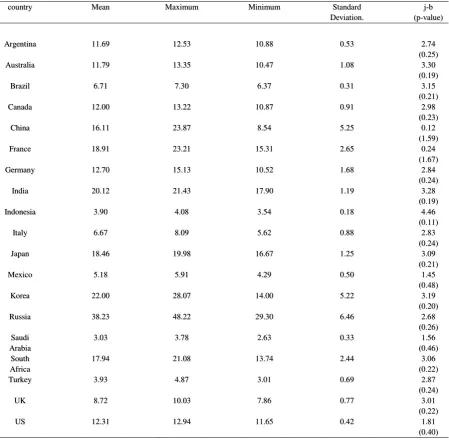
from 1990 to 2016. The data is reported as suicides per 100,000 people and Table 1 presented
the descriptive statistics of each of the countries. In examining the overall global trends in
suicide mortality rate, our empirical data suggests that on average, approximately 830,883
people die annually from suicide worldwide from 1990 – 2016. This corresponds to an
age-standardised suicide mortality rate of about 14.3 per 100 000 people over the period. In 2016,
approximate 817 147 people died from suicide worldwide compared to 766 043 in 1990. This
A cursory look at the trends in the time series data for G20 countries indicates that the
prevalence of suicide mortality varies considerably across countries and over time. We
particularly note that the highest suicide averages are found in 4 out of the 5 members of the
BRICS alliance of countries (Russia (38.23), India (20.12), China (16.11), South Africa
(17.91)) as well as for Japan (18.46) and Korea (22.00) which are East Asian economies. On
the other hand, lower, single digit suicide averages are more prominent within Saudi Arabia
(3.03) as a “Middle-East” representative; the three ‘G20 members’ of the MINT group of
emerging economies (Mexico (5.18), Indonesia (3.90) and Turkey (3.93)); the South
American countries of Brazil (6.71) as well as for Italy (6.67) and the UK (8.72). Finally,
intermediate, double digit averages of suicide rates are found in the remaining economies
which are largely G7 and Latin American countries (Argentina (11.69), Australia, (11.79),
Canada (12.00), US (12.31), Germany (12.70), France (18.91)). Note that these observations
are somewhat contrary to conventional academic wisdom which speculates on suicide
mortality being more prevalence in emerging and less developed countries than in developed
countries due to the socioeconomic and behavioural factors, limited access to mental health
care and shortage of behavioural health care providers (Moneim et al. (2011); Kumar et al.
Table 1: Descriptive statistics
country Mean Maximum Minimum Standard Deviation.
j-b (p-value)
Argentina 11.69 12.53 10.88 0.53 2.74 (0.25) Australia 11.79 13.35 10.47 1.08 3.30
(0.19) Brazil 6.71 7.30 6.37 0.31 3.15
(0.21) Canada 12.00 13.22 10.87 0.91 2.98
(0.23) China 16.11 23.87 8.54 5.25 0.12
(1.59) France 18.91 23.21 15.31 2.65 0.24
(1.67) Germany 12.70 15.13 10.52 1.68 2.84
(0.24) India 20.12 21.43 17.90 1.19 3.28
(0.19) Indonesia 3.90 4.08 3.54 0.18 4.46
(0.11) Italy 6.67 8.09 5.62 0.88 2.83
(0.24) Japan 18.46 19.98 16.67 1.25 3.09
(0.21) Mexico 5.18 5.91 4.29 0.50 1.45
(0.48) Korea 22.00 28.07 14.00 5.22 3.19
(0.20) Russia 38.23 48.22 29.30 6.46 2.68
(0.26) Saudi
Arabia
3.03 3.78 2.63 0.33 1.56 (0.46) South
Africa
17.94 21.08 13.74 2.44 3.06 (0.22) Turkey 3.93 4.87 3.01 0.69 2.87
(0.24)
UK 8.72 10.03 7.86 0.77 3.01
(0.22) US 12.31 12.94 11.65 0.42 1.81
(0.40)
Notes: Authors own computation. j-b statistic indicates that all series are normally
distributed.
Figure 1 depicts the evolution of suicide mortality rate per 100 000 people for period
1990 – 2016 among the G20 members. While most countries do not exhibit clear trends, it is
evident that suicide mortality rate has progressively declined over time except for the
Republic of Korea and to some extent the Kingdom of Saudi Arabia and the United States.
However, there are two noticeable trends in suicide mortality over the periods. First, there
were spikes in suicide mortality in a number of countries such as Argentina, Australia, Japan,
1997 – 2000. This period coincides with the periods of economic crises such as the Asian
currency crisis of 1997, the Russian default crisis of 1998, and Turkish crisis of 2000
(Asongu, 2012). Another notable trend was around the global financial crisis of 2007/08 in
which countries such as Mexico, Republic of Korea, Saudi Arabia and Turkey experienced
increase in suicide mortality over this period. These represent important structural break
[image:17.595.73.523.237.513.2]points which need to be accounted for in our empirical analysis.
Figure 1: Suicide mortality rate per 100 000 people, 1990 – 2016
10.8 11.2 11.6 12.0 12.4 12.8
1990 1995 2000 2005 2010 2015
Argentina 10 11 12 13 14
1990 1995 2000 2005 2010 2015
Australia 6.2 6.4 6.6 6.8 7.0 7.2 7.4
1990 1995 2000 2005 2010 2015
Brazil 10.5 11.0 11.5 12.0 12.5 13.0 13.5
1990 1995 2000 2005 2010 2015
Canada 8 12 16 20 24
1990 1995 2000 2005 2010 2015
China 14 16 18 20 22 24
1990 1995 2000 2005 2010 2015
France 10 11 12 13 14 15 16
1990 1995 2000 2005 2010 2015
Germany 17 18 19 20 21 22
1990 1995 2000 2005 2010 2015
India 3.5 3.6 3.7 3.8 3.9 4.0 4.1
1990 1995 2000 2005 2010 2015
Indonesia 5.5 6.0 6.5 7.0 7.5 8.0 8.5
1990 1995 2000 2005 2010 2015
Italy 16 17 18 19 20 21
1990 1995 2000 2005 2010 2015
Japan 12 16 20 24 28 32
1990 1995 2000 2005 2010 2015
Korea 4.0 4.5 5.0 5.5 6.0
1990 1995 2000 2005 2010 2015
Mexico 25 30 35 40 45 50
1990 1995 2000 2005 2010 2015
Russia 12 14 16 18 20 22
1990 1995 2000 2005 2010 2015
SA 2.4 2.8 3.2 3.6 4.0
1990 1995 2000 2005 2010 2015
Saudi 2.5 3.0 3.5 4.0 4.5 5.0
1990 1995 2000 2005 2010 2015
Turkey 7.5 8.0 8.5 9.0 9.5 10.0 10.5
1990 1995 2000 2005 2010 2015
UK 11.6 12.0 12.4 12.8 13.2
1990 1995 2000 2005 2010 2015
US
Data source: IHME, Global Burden of Disease
5 EMPIRICAL RESUTLS
5.1 First generation unit root test results
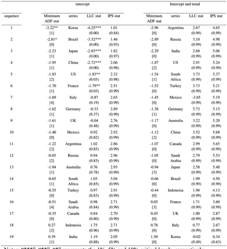
Table 2 presents the results of the SPSM approach applied to the cluster of first
generation unit root tests, with Panel A reporting the results of the procedure performed on
the pairs of unit root tests with a drift and Panel B showing the results for the procedure
performed on pairs of unit roots performed with both a drift and trend. To carry out the
and report the results in a sequential format, with the series with the highest rejection or
lowest test statistic being reported first (in our case is Korea when the tests are performed
with a drift and Argentina when the tests are performed with both drift and trend) followed by
the series with the second highest rejection ‘test statistic’ (which is now Brazil for the drift
models and Russia for the drift and tend model) and so forth.
We then perform the panel unit root tests (LLC and IPS tests) in a similar sequential
fashion, with the first panel test statistic computed for the entire panel, then the second panel
statistic computed for the panel with the individual series yielding the highest rejection being
removed from the panel, then the third panel statistic is computed for the panel with the
individual series yielding the highest and second highest rejection rates being removed from
the panel, and this procedure is carried out in this fashion of a consecutively reducing panel
until we have segregated the stationary from the non-stationary panel. The optimal lag for
each of the performed tests is determined by the minimization of the modified AIC as
suggested by Ng and Perron (1996, 2001). The results show some discrepancies in results
obtained. For instance, when the procedure is carried out with a drift, the LLC statistic
identifies 6 stationary processes (i.e. Korea, Brazil, Japan, china, US and France) whereas the
IPS statistics find no stationary series. On the other hand, when the procedure is carried out
with a drift inclusive of a trend, none of the individual or panel statistics identified any
stationary processes. Nevertheless, we cannot consider these results as conclusive since they
ignore important nonlinearities and structural breaks found in the data. We address these
Table 2: SPSM applied to first generation unit root tests
intercept Intercept and trend
sequence Minimum ADF stat
series LLC stat IPS stat Minimum ADF stat
series LLC stat IPS stat
1 -3.22** [1]
Korea -4.25*** (0.00)
1.01 (0.84)
-2.96 [0]
Argentina 2.67 (0.99)
4.65 (0.99) 2 -2.81*
[0]
Brazil -3.32*** (0.00)
1.46 (0.93)
-2.89 [0]
Russia 3.10 (0.99)
4.98 (0.99) 3 -2.23
[1]
Japan -2.83*** (0.00)
1.82 (0.97)
-2.29 [0]
India 2.68 (0.99)
5.06 (0.99) 4 -1.95
[1]
China -2.72*** (0.00)
2.06 (0.98)
-1.87 [2]
US 2.91 (0.99)
5.24 (0.99) 5 -1.83
[2]
US -1.83** (0.03) 2.32 (0.98) -1.54 [1] South Africa 3.73 (0.99) 5.37 (0.99) 6 -1.70
[1]
France -1.79** (0.03)
2.51 (0.99)
-1.52 [0]
Turkey 3.73 (0.99)
5.21 (0.99) 7 -1.69
[4]
Italy -0.87 (0.19)
2.65 (0.99)
-1.45 [0]
Mexico -3.65 (0.99)
5.19 (0.99) 8 -1.62
[1]
Germany -0.33 (0.37)
2.89 (0.99)
-1.38 [1]
Germany 5.73 (0.99)
5.15 (0.99) 9 -1.61
[1]
UK -0.04 (0.48)
2.76 (0.99)
-1.17 [0]
Australia 3.22 (0.99)
5.20 (0.99) 10 -1.40
[0]
Mexico 0.92 (0.82)
2.92 (0.99)
-1.12 [2]
China 3.52 (0.99)
5.68 (0.99) 11 -1.22
[2]
Argentina 1.02 (0.85)
2.86 (0.99)
-1.07 [0]
Canada 2.99 (0.99)
5.65 (0.99) 12 -0.85
[2]
Russia 0.94 (0.83) 2.96 (0.99) -1.05 [0] Saudi Arabia 2.79 (0.99) 5.53 (0.99) 13 -1.04
[1]
Australia 0.76 (0.78)
2.93 (0.99)
-0.94 [3]
Japan 2.58 (0.99)
5.40 (0.99) 14 -0.65
[1] South Africa 1.03 (0.85) 3.04 (0.99) -0.66 [0]
Brazil 1.99 (0.99)
4.50 (0.99) 15 -0.55
[0]
Turkey 0.97 (0.83)
2.91 (0.99)
-0.44 [0]
Indonesia 1.96 (0.99)
4.13 (0.99) 16 -0.51
[4] Saudi Arabia 0.98 (0.84) 2.71 (0.99) 0.05 [3]
France 1.71 (0.99)
3.60 (0.99) 17 -0.35
[0]
Canada 0.84 (0.80)
2.70 (0.99)
0.45 [0]
UK 1.00 (0.99)
2.87 (0.99) 18 0.27
[2]
Indonesia 1.75 (0.96)
2.71 (0.99)
0.78 [0]
Italy 0.77 (0.99)
2.67 (0.99) 19 0.39
[1]
India 1.19 (0.88)
2.05 (0.99)
1.50 [0]
Korea -0.02 (0.49)
0.34 (0.63)
Notes: “***”, “**”, “*” represents the 1%, 5% and 10% critical levels, respectively.
5.2 Second generation unit root test results
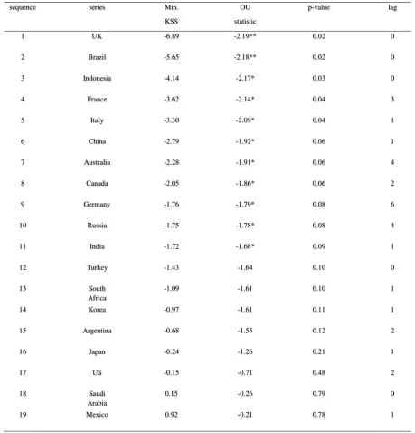
Table 3 presents the results of the SPSM approach applied to our second-generation
unit root tests of KSS (2003) and Omay and Ucar (2009). As before we begin the process by
computing the individual KSS statistic for each of the individual series, which are reported in
The sequences as well as the estimated values of these individual statistics are found in the
first three columns of Table 3. Thereafter, we apply the OU sieve bootstrap procedure in
order to compute the corresponding OU panel statistic, firstly for the entire panel, and then on
a reducing panel set in which individual series with the highest rejection are sequentially
removed until we effectively segregate the stationary from the non-stationary panel. These
panel unit root statistics are reported in the fourth column of Table 3 whilst the bootstrap
p-values and the associate optimal lags lengths are found in the fifth and sixth columns of Table
3, respectively.
After completing the procedure, we find the panel of stationary time series for 11 of
the G20 countries (the United Kingdom, Brazil, Indonesia, France, Italy, China, Australia,
Canada, Germany, Russia and India) whereas the remaining countries (Turkey, South Africa,
Korea, Argentina, Japan, the United States, Saudi Arabia and Mexico) exhibit non-stationary
behaviour. Interestingly enough, the stationary panel consists of 6 advanced and 5 emerging
economies of the G20 panel whereas the non-stationary panel primarily consists of emerging
non-G7 member states. We also note that these results can also be compared to those
obtained in the previous study of Chang et al. (2017) who use a similar SPSM framework
applied to a sample of 23 OECD countries of which 6 of these countries (The United
Kingdom, France, Italy, Canada, Japan and the United States) belong to our panel of G20
countries. However, in differing from Chang et al. (2017) who find unit root behaviour for all
these ‘commonly sampled’ economies, our current findings point to stationarity in 5 out of
Table 3: SPSM approach to second generation unit root tests
sequence series Min. KSS
OU statistic
p-value lag
1 UK -6.89 -2.19** 0.02 0
2 Brazil -5.65 -2.18** 0.02 0
3 Indonesia -4.14 -2.17* 0.03 0
4 France -3.62 -2.14* 0.04 3
5 Italy -3.30 -2.09* 0.04 1
6 China -2.79 -1.92* 0.06 1
7 Australia -2.28 -1.91* 0.06 4
8 Canada -2.05 -1.86* 0.06 2
9 Germany -1.76 -1.79* 0.08 6
10 Russia -1.75 -1.78* 0.08 4
11 India -1.72 -1.68* 0.09 1
12 Turkey -1.43 -1.64 0.10 0
13 South Africa
-1.09 -1.61 0.10 1
14 Korea -0.97 -1.61 0.11 1
15 Argentina -0.68 -1.55 0.12 2
16 Japan -0.24 -1.26 0.21 1
17 US -0.15 -0.71 0.48 2
18 Saudi Arabia
0.15 -0.26 0.79 0
19 Mexico 0.92 -0.21 0.78 1
Notes: “***”, “**”, “*” represents the 1%, 5% and 10% critical levels, respectively. p-values
for OU statistic generated through a bootstrap of 10,000 replications.
5.3 Third generation unit root test results
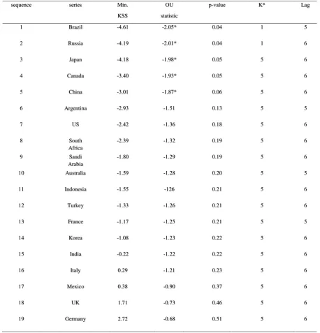
Table 4 presents the results for the results for the SPSM applied to the third
generation unit root testing procedure. These tests vary from the first and second generation
intended to capture a series of unobserved, smooth structural breaks and have been
demonstrated to be more powerful than other structural breaks or nonlinear unit root tests
(Becker et al. (2006) and Enders and Lee (2012)). Recall, that the procedure is cried by firstly
estimating individual KSS-FFF test statistics for the individual countries and then these test
statistics are arranged in order of lowest to the highest values. The results of this exercise are
reported in the first three columns of Table 4. Thereafter the OU bootstrap procedure is
carried out as previously, firstly for the whole panel, then on a reducing panel in which the
KSS-FFF statistic with the highest rejection is sequentially removed in each stage of the
estimation process.
The obtained panel statistics are found in the fourth column of Table 4 and the
bootstrap p-values are given in the fifth column of the same table, whereas the findings of the
grid search to identify the optimal frequency component, k*, and lag length, are reported in
columns 6 and 7 of Table 4, respectively. In a nutshell, our results point to a stationary of
panel of countries inclusive of Brazil, Russia, Japan, Canada and China, whilst the
non-stationary panel consists of Argentina, the United States, South Africa, Saudi Arabia,
Australia, Indonesia, Turkey, France, Korea, India, Italy, Mexico, the United Kingdom and
Germany. Notice that the stationary panel is smaller than that obtained for the KSS test
performed without a FFF approximation, and this panel consists of 3 of the BRICS member
states and two G7 member states. Further note that these findings are now more similar to
those of Chang et al. (2017), who also find that by including a FFF approximation in the
testing procedure, most industrialized countries fall under the non-stationary panel of
suicides. Overall, these findings highlight the importance of accounting for both
nonlinearities and smooth structural breaks in distinguishing stationary from non-stationary
Table 4: SPSM approach to second generation unit root tests
sequence series Min. KSS
OU statistic
p-value K* Lag
1 Brazil -4.61 -2.05* 0.04 1 5
2 Russia -4.19 -2.01* 0.04 1 6
3 Japan -4.18 -1.98* 0.05 5 6
4 Canada -3.40 -1.93* 0.05 5 6
5 China -3.01 -1.87* 0.06 5 6
6 Argentina -2.93 -1.51 0.13 5 5
7 US -2.42 -1.36 0.18 5 6
8 South Africa
-2.39 -1.32 0.19 5 6
9 Saudi Arabia
-1.80 -1.29 0.19 5 6
10 Australia -1.59 -1.28 0.20 5 5
11 Indonesia -1.55 -126 0.21 5 6
12 Turkey -1.33 -1.26 0.21 5 6
13 France -1.17 -1.25 0.21 5 5
14 Korea -1.08 -1.23 0.22 5 6
15 India -0.22 -1.22 0.22 5 6
16 Italy 0.29 -1.21 0.23 5 6
17 Mexico 0.38 -0.90 0.37 5 6
18 UK 1.71 -0.73 0.46 5 6
19 Germany 2.72 -0.68 0.51 5 6
Notes: “***”, “**”, “*” represents the 1%, 5% and 10% critical levels, respectively. p-values
for OU statistic generated through a bootstrap of 10,000 replications.
6 CONCLUSION
Primarily motivated by the lack of empirical evidence due to the novelty of the field
in research study, we have investigated the possibility of persistence in suicides in G20
by the World Health Organization (WHO) as one of the leading causes of mortalities
globally. The selection of the G20 countries as a case study is important since these countries
are currently the centre of global economic dominance and hence the potential influence of
these countries in reducing global suicides cannot be overlooked or taken for granted.
Previous studies have examined possible persistence in suicides for the US and OECD
countries hence lacking global outlook on the subject matter. Our sample covers a period of
1996 to 2017 since this is the longest and most consistent data collectively available for
empirical use from various databases. Empirically we rely on the SPSM approach of
Chortareas and Kapetanois (2009) which we apply to three generations of unit root tests
(those being the i) conventional unit root tests ii nonlinear unit root tests iii) FFF-based
nonlinear unit root tests). After controlling for nonlinearities and smooth structural breaks in
the data, we find that only Brazil, Russia, Japan, Canada and China have stationary suicides
whilst we fail to find any convincing evidence of stationarity amongst the remaining
countries, which comprises mainly of industrialized, G20 member states.
There are some important policy implications which can be gathered from our
findings. For starters, we concur with the World Organization and particularly advise that
G20 countries should move toward adoption of formal national suicide prevention strategies
which are tailored according to each of the members social, religious and economic
standards. Other non-G20 countries could then ‘copy’ the strategies implemented by G20
countries by identifying with member states which best correspond with their social,
economic, religious and regional standings. Such proposed suicide prevention strategies
should primarily emulate from health and social ministries within each economy and should
then be spread across different sectors of the economy, primarily the health care sector,
business sector, education sector (primary, secondary and tertiary levels of education) as well
within local communities. As detailed in the “Mental Health Plan” report of the World
Health Organization (2013) prevention strategies could include surveillance measures, means
restrictions, media guidelines, stigma reduction as well as public awareness and training.
From an empirical standpoint, a comprehensive system of adequate data collection
should be put into place by G20 as well non-G20 member states which can provide a rich
source of suicide numbers across the different sexes, races, age groups, religious backgrounds
and other relevant socio-demographic factors. This would require more rigid data-collecting
institutional structures dedicated towards collecting and processing such time series which
would in turn naturally enrich the future academic path of research on suicides as well as
forecasting practices not only for G20 countries but other less researched recognized
economies in less developed regions of the world. However, with the currently available data,
one possible avenue for the near-future research would be to extend upon the current
knowledge on the so-called “natural-rate of suicides” literature which can be perceived as a
natural extension of the knowledge gained from investigating the persistence of suicides.
REFERENCES
Andres A. (2005), “Income equality, unemployment and suicide: a panel data analysis of 15
European countries”,Applied economics, 37(4), 439-451.
Andres A. and Halicioglu F. (2011), “Testing the hypothesis of the natural suicide rates: Further evidence from OECD data”, Economic Modelling, 28(1-2), 22-26.
Asongu S. (2012), “Globalisation, financial crisis and contagion: time-dynamic evidence
from financial markets of developing countries”, MPRA paper no 37572.
Brainerd E. (2001), “Economic reform and mortality in the former Soviet Union: A study of
the suicide epidemic in the 1990s”,European Economic Review, 87(4-6), 1007-1019.
Campbell J. and Mankiw G. (1987), “Are output fluctuations transitory?”, The Quarterly
Case A. and Deaton A. (2015), “Suicide, age, and wellbeing: An empirical investigation”,
NBER Working Paper No. 21279, June.
Chang S., Stuckler D., Yip P. and Gunnell D. (2013), “Impact of the 2008 global economic crisis on suicide: Time trend study in 54 countries”, British Medical Journal, 347(f5239),
1-15.
Chang T., Cai Y. and Chen W. (2017), “Are suicide rate fluctuations transitionary or
permanent? Panel KSS unit root test with a Fourier function through the sequential panel
selection method”, Romanian Journal of Economic Forecasting, 20(3), 5-17.
Chen W., Chang T. and Lin Y. (2018), “Investigating the persistence of suicide in the United States: Evidence from the quantile unit root test”, Social Indicators Research, 135(2),
813-833.
Chortareas G. and Kapetanois G. (2009), “Getting PPP right: Identifying mean-reverting real
exchange rates in panels”, Journal of Banking and Finance, 30(2), 390-404.
Chu X., Zhang X., Cheng P., Schwebel D. and Hu G. (2018), “Assessing the use of media
reporting recommendations by the World Health Organization in suicide news published in
the most influential media sources in China, 2003-2015”, International Journal of
Environmental Research and Public Health, 15(451), 1-12.
Chuang H. and Huang W. (1997) “Economic and social correlates of regional suicide rates: A
pooled cross-section and time-series analysis”,Journal of Socio-Economics, 26(3), 277-289.
Dahlberg M. and Lundin D. (2005), “Antidepressants and the suicide rate: Is there really a
Daly M., Oswald A., Wilson D. and Wu S. (2013), “Dark contrasts: the paradox of high rates
of suicides in happy places”, Journal of Economic Behaviour and Organization, 80(3),
435-442.
Durkheim, E. 1987. Suicide. Translated by Spaulding, J and Simpson, G. Reprinted Glencore,
III: Free Press, 1951.
Enders and Lee (2012), “A unit root test using a Fourier series to approximate smooth breaks”, Oxford Bulletin of Economics and Statistics, 74(4), 574-599.
Institute of Health Metrics and Evaluation (2018). Global Burden of Disease (GBD) database.
Ginsberg R. (1966), “Anomic and aspiration: a reinterpretation of Durkeim’s theory”,
Dissertation. New York.
Hamermesh D. and Soss N. (1974), “An economic theory of suicide”, Journal of Political
Economy, 82(1), 83-98.
Henry, A. and Short, J. 1954. Suicide and homicide. Glencore, III: Free Press.
Im K., Pesaran M. and Shin Y. (2003), “Testing for unit roots in heterogeneous panels”,
Journal of Econometrics, 115(1), 53-74.
Jusufbegovic, J. and Ottoson, J. 2011. Understanding suicide: a socio-economic approach.
Master’s thesis: Lingkoping University, Department of Engineering and Management.
Kegler S., Stone D. and Holland K. (2017), “Trend in suicide by level of urbanization –
Kumar S., Verma A., Bhattacharya S. and Rathore, S. (2013), “Trends in rates and methods
of suicide in India”,Egyptian Journal of Forensic Sciences, 3(3), 75-80.
Lee L., Roser M., and Ortiz-Ospina E., (2015). Suicide. Retrieved June 8, 2018, from:
http://ourworldindata.org/suicide
Lee J. and Strazicich M. (2004), “Minimum Lagrange multiplier unit root with two structural
breaks”, The Review of Economics and Statistics, 85(4), 1082-1089.
Lee J. and Strazicich M. (2013), “Minimum LM unit root with one structural break”,
Economics Bulletin, 33(4), 2483-2493.
Levin A., Lin C. and Chu J. (2002), “Unit root tests in panel data: asymptotic and
finite-sample properties”, Journal of Econometrics, 108(1), 1-24.
Maddala G. and Wu S. (1999), “A comparative study of unit root tests with panel data and a new simple test”, Oxford Bulletin of Economics and Statistics, 61(51), 631-652.
McKinnon J. (1994), “Approximate asymptotic distribution functions for unit-root and
cointegration tests”, Journal of Business and Economic Statistics, 12(2), 167-176.
Minoiu C. and Andres A. (2008), “The effect of public spending on suicide: Evidence from US State data”, The Journal of Socio-Economics, 37, 237-261.
Moneim W., Yassa H. and George S. (2011), “Suicide rate: trends and implications in Upper
Egypt”,Egyptian Journal of Forensic Sciences, 1(1), 48 – 52.
Neumayer E. (2003), “Socio-economic factors and suicide at large unit aggregate levels: a
comment”, Urban studies, 40(13), 2769-2796
Oblander E., Sojung P. and Lemaire J. (2016), “The cost of high suicide rate in Japan and
Republic of Korea: reduced life expectancies”, Asia-Pacific Population Journal, 31(2), 21 –
24.
Perron P. (1989), “The great crash, the oil price shock, and the unit root hypothesis”,
Econometrica, 57(6), 1361-1401.
Phiri A. and Mukuku D. (2017), “Does unemployment aggravate suicide rates in South Africa? Some empirical evidence”, MPRA Working Paper No. 80749, August.
Platt S. (1984), “Unemployment and suicidal behaviour: A review of the literature”, Social
Science and Medicine, 19(2), 93-115.
Platt S., Micciolo R. and Tansella M. (1992), “Suicide and unemployment in Italy:
Description, analysis and interpretation of recent trends”, Social Science and Medicine,
34(11), 1191-1201.
Viren M. (1999), “Testing the “natural rate of suicide” hypothesis”, International Journal of
Social Economics, 26(12), 1428-1440.
World Health Organisation (2018). World Health Statistics database.
Yang B. and Lester D. (1991), “Is there a natural suicide rate for society?”, Psychological
Reports, 68, 322.
Yang B. and Lester D. (2009), “Is there a natural suicide rate?”, Applied Economic Letters,
Yeh B. and Lester D. (1987), “An economic model for suicide: In David Lester (Ed.)”,
Suicide as a learned behaviour, Springfield, Illinois.
Zivot and Andrew (1992), “Further evidence on the Great Crash, the oil-price shock, and the