Heap hot spots visualization in Java

Heap Hot Spots Visualization in Java

Babak Mahdavi

School of Computer Science McGill University

[email protected]

Karel Driesen

School of Computer Science McGill University

[email protected]

ABSTRACT

Data memory (heap) management is a particularly important feature of the Java programming environment. The visualization of memory location in form of hot spots can help to see how the data cache is used during the execution of a program. The behavior of such executed program can be thus speculated. Through a series of experiments using Load and Store trace files, some pertinent aspect of data memory accessing, can be visualized, including the frequency of how often the Java virtual machine references class variable addresses. A demonstration will be included showing how object variables are accessed in the heap by allowing one to visualize (X, Y) graph hot spots.

1. INTRODUCTION

The Effective Addresses (EA) can be defined as the address that one can load data from or store to. They reveal how many times one loads from (or stores to) a used location. The behavior of Effective Addresses is visualized as hot spots throughput the execution of the seven benchmark utilities (SPECJVM98)and a ray tracing program called “raytrace”. A program hot spot is a collection of instructions which are executed repeatedly, typically in an inner loop of some program phase. The size of a hot spot indicates the minimum size of an instruction cache that is able to execute all instructions without encountering cache capacity misses. Hot spots are also important in other domains than instruction addresses, such as load/store addresses (Data Cache) [1]. The purpose of this paper is to demonstrate the results of a case study (load/store) in which such hot spots can be located in an easy and practical way, for the execution of a given suite of programs running on the Java Virtual Machine. In the context of this case study, Effective Address will be used to denote an address referenced (or informally “touched”) by a load or store instruction. It will be of interest to track the frequency of EA referenced over certain time intervals 1.The behavior of EAs can be thus visualized as hot spots across the execution of these seven benchmark utilities and the ray tracing program.

2. METHODOLOGY

Standard Performance Evaluation Corporation (SPEC) [2] provides SPECJVM98 benchmarks which measure the

1

one reason that such as study would be of value is that it may be possible to identify certain program code segments from the hot spots, on which the careful application of a dynamic optimizing compiler could reduce the (overall) runtime of the given program.

performance of Java virtual machines2. Table 1. shows a brief description of SPECJVM98 benchmark suite. The Load/Store traces files were collected (generated by Kaffe 3 [3]) from graduate course on Adaptivity in Computational Systems (CS764 2000). The experimental procedure is shown in Figure 1.

Table 1. The SPECjvm98 benchmark suite

check A program developed by SPEC to check JVM and Java features. (Not Used)

compress A popular LZW compression program.

jess

A Java version of NASA's popular CLIPS rule-based expert system, licensed from Sandia Laboratories.

db Data management benchmarking software written by IBM.

javac The JDK Java compiler licensed from Sun Microsystems.

mpegaudio

The core algorithm for software that decodes an MPEG-3 audio stream; licensed from Fraunhofer Institut fuer Integrierte Schaltungen.

mtrt A dual-threaded program that ray traces an image file.

jack A real parser-generator licensed from Sun Microsystems.

2

SPECjvm 98 measures the time it takes to load the program, verify the class files, compile on the fly if JIT compiler is used, and execute the test. From the software perspective, these tests measure the efficiency of the JVM, JIT compiler and operating system implementations on a given hardware platform. From the hardware perspective, the benchmark measure CPU, cache, memory and other platform specific hardware performance. A 24MB heap is sufficient to run all the benchmark tests. AWT, network, database, and graphics performance are not measured by the benchmark.

3

Figure 1. Experimental Procedure

Plumber 3.04

DataToPs

Load/Store trace file generated by Kaffe

Resulting Hot Spots data file

post script file

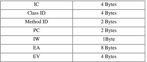
The breakdown of the format of the tracing byte codes files are summarized in Table 2.

§ Instruction Counter (IC) : Number of instructions since program start.

§ Class ID: the id of the class.

§ Method ID: the id of the method.

§ Program Counter (PC): address of instruction.

§ Instruction Word (IW): value of byte code.

§ Effective Address (EA): addresses where data are loaded from or stored to.

§ Effective Value (EV): value that is loaded or stored.

Table 2. Architecture of the trace byte codes information

IC 4 Bytes

Class ID 4 Bytes Method ID 2 Bytes

PC 2 Bytes

IW 1Byte

EA 8 Bytes

EV 4 Bytes

The Effective Addresses are re-numbered using the id-dispenser4 implemented in Plumber 3.04 [4]. The first memory location referenced is denoted by the number 1, the second 2 , and so on. Every EA is looked up in a table that maps EA to this number. If an EA is absent from the table, it receives the next number and is inserted in the table. This re-numbering scheme has several benefits for hot spot visualization purposes:

§ space on the Y-axis is better used, since every number has at least one sample in which it appears (there are no blank horizontals). In contrast, real memory location touched leave a wide unused horizontal gaps in the graphs.

§ Two runs of the same program on different machines will look different when real addresses are used. Re-numbering ensures that identical runs have identical profiles, and therefore renders a platform-independent visualization [1].

3. VISUALISATION

Only the first 2,000,000 instructions are traces for each Load/Store byte codes trace file and measurements are reported over sample of 20,000 instructions (yielding 100 data points per trace). The X and Y axis are defined as following:

§ X-axis: Time, Byte code execution in sample of 20,000.

§ Y-axis: Location, Re-numbered memory locations loaded or store in sample.

Table 3. shows the Y maximum values for every executed program.

Table 3. Max values for Y-axis obtained in each executed byte code trace

Program Name Y (Max)

raytrace 33209

compress 96089

jess 24396

db 79374

javac 28825 mpegaudio 47405 mtrt 33221 jack 13209 4

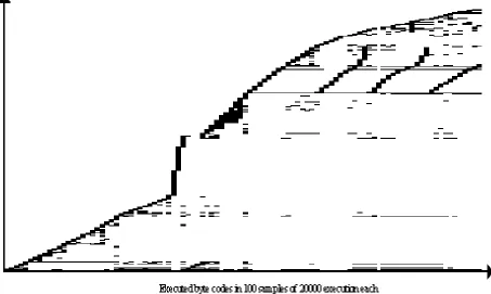
Figure 2 shows hot spots in memory addresses referenced by loads and stores in the execution of javac program. Hot spots seem to be small (thin rectangles), but the program seems to touch large parts of the memory only once. In the second half of the trace, repeated iterations over the same memory locations appear as slanted lines [1]. These memory locations touched

within a sample on Y-axis are re-numbered effective values. It is important to mention that these values are IDs and they can just reveal which ones of these addresses are accessed first. However, they do not present the real memory location. For instance, one can not conclude that a specific part of memory (e.g. lower part or higher part) is accessed first or second.

Figure 2. JAVAC-Load/Stores: memory locations referenced in first 2M byte codes of javac

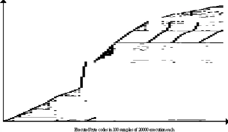
Figure 3 shows only the loads hot spots referenced in the same program. The repeated iterations over the same memory locations which appear as slanted lines are effectively loads operations since these iterations do not appear on the store graph presented in Figure 4. The overlap between these two graphs is justified: The Instruction Words (value of byte codes in this

Figure 3. JAVAC-Loads: memory locations referenced in first 2M byte codes of javac

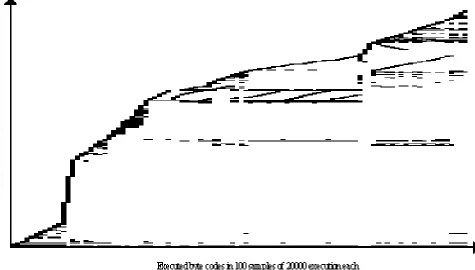
Data cache touched hot spots in the execution of jess program is shown in Figure 5. The initiation part is shorter comparing to javac but there are still repeated iterations over the same memory location, appears in thinner rectangle this time as it can

be seen in Figure 6, most referenced EA are loads. Stores can be seen in Figure 7.

Figure 5. JESS-Load/Stores: memory locations referenced in first 2M byte codes of jess

Figure 7. JESS-Stores: memory locations referenced in first 2M byte codes of jess

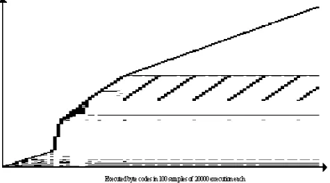
In mtrt which is multi-threaded ray tracing program, these repeated loops are repeated over a long period of time. It is also possible to see that a particular location of the memory is

constantly accessed (right above and under repeated loops) during these loops as well as new accessed memory area progressively increasing during the same time (see Figure 8).

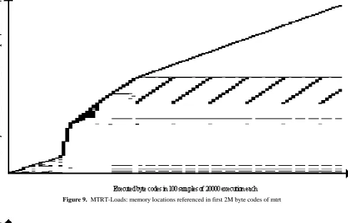
By comparing Figure 9 and Figure 10 with Figure 8, it can be observed that those long repeated loops are actually the loads

operations.

Figure 9. MTRT-Loads: memory locations referenced in first 2M byte codes of mtrt

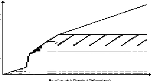
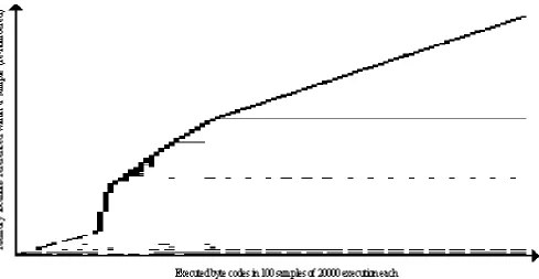
It is not surprising to see in Figure 11 that the execution of the raytrace program hot spots looks extremely similar to mtrt (however not exactly the same). After all, mtrt is the same

raytracing program but mutli-threaded. See Figure 12 and Figure 13 for RAYTRACE-Loads and RAYTRACE-Stores.

Figure 11. RAYTRACE-Load/Stores: memory locations referenced in first 2M byte codes of raytrace

Figure 13. RAYTRACE-Stores: memory locations referenced in first 2M byte codes of raytrace

In the last phase of the mpegaudio program (Figure 14), two different parts of the memory location are touched almost identically for their respective period time. By looking at Figure

14 and Figure 16, it appears that these locations have been referenced by Loads.

Figure 15. MPEGAUDIO-Loads: memory locations referenced in first 2M byte codes of mpegaudio

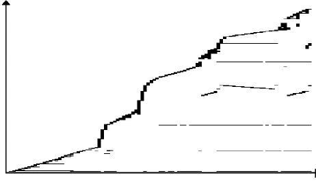
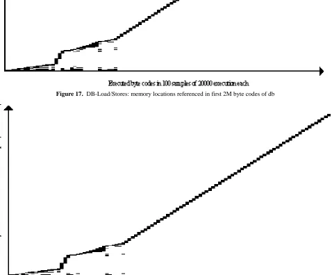
In second half of the execution of db program (Figure 17), the hot spots trace shows how memory is referenced continually over the time and never accessed for a second time. A quick

look at Loads and Stores (Figure 18 and Figure 19 respectively), would be enough to realize that these Effective Addresses have been referenced by both read and write operations.

Figure 17. DB-Load/Stores: memory locations referenced in first 2M byte codes of db

Figure 19. DB-Stores: memory locations referenced in first 2M byte codes of db

However as for jack (Figure 20), there are also some memory locations that are touched constantly during the second half of the trace. These are mostly loads but also stores. For instance, the combination of the forth dashed line (above x-axis) in

JACK-Loads (Figure 21) and JACK-Stores (Figure 22) can be seen as a thick line appears in Figure 20 (JACK-Load/Stores ) on the fifth line. Using some transparencies can help to see more clearly this mapping once they are superimposed.

Figure 21. JACK-Loads: memory locations referenced in first 2M byte codes of jack

Finally, during the third part of the execution of the compress program shown in Figure 23, a huge part of memory location are referenced particularly on the upper part of the trace. This is because of the result of reading Effective Addresses as it can be

clearly seen in Loads (Figure 24). COMPRESS-Stores (Figure 25) shows that compress program is probably the one that is dominated by the stores operations

Figure 23. COMPRESS-Load/Stores: memory locations referenced in first 2M byte codes of compress

Figure 25. COMPRESS-Stores: memory locations referenced in first 2M byte codes of compress

4. CONCLUSION AND FUTURE WORK

A visualization technique for detecting hot spots in Java heap (data cache) using Loads/Stores instruction in different programs was traced and demonstrated. The Loads and Stores have been also showed separately in order to see which hot spots present actually reading from EAs (loads) and which ones writing to EAs (stores). In most cases, loads seem to be dominant except for db for which there are as much as stores than loads and also compress which has more store operations. For better visualization of these hot spots and also having an independent platform encoding values, re-numbering scheme was used. These hot spots do not reveal the actual physical location in memory but rather the order in which they have been loaded from or stored to. As a result of this study, it could be suggested that some of the most commonly used areas in the heap, are better suited to be cached for faster accessibility thus better performance. A use of color is planned for the future work.

5. ACKNOWLEDGMENTS

Thanks to Nagi Basha for his contribution to this project.

6. REFERENCES

[1] Karel Driesen, Nagi Basha, David Eng, Matt Holly, John Jorgensen, Georges Kanaan, Babak Mahdavi, Qin Wang. Visualizing Hot Spots in Various Domains. Software Visualization Workshop at ICSE ( Toronto, ONT, May 2001)

[2] The Standard Performance Evaluation Corporation,

http://www.spec.org/

[3] Kaffe, http://www.kaffe.org/