Fuzzy Modeling using Vector Quantization based
on Input and Output Learning Data
Hirofumi Miyajima, Noritaka Shigei, and Hiromi Miyajima
Abstract—Many studies on fuzzy modeling(learning of fuzzy inference systems) with vector quantization(VQ) and steepest descend method (SDM) have been made. It is known that these methods are superior in the number of rules(parameters) compared with other learning methods. Most of conventional learning methods using VQ are ones that determine initial assignment of center parameters for membership functions in antecedent part using only input part of learning data, initial assignment of center parameters for membership functions in antecedent part using all learning data and the initial assignment of all parameters in systems using VQ and the generalized onverse matrix(GIM). These methods are ones that determine the initial assignment of parameters in learning process, and any learning data in learning steps of SDM is selected randomly. On the other hand, it is known that many fuzzy rules are needed at or near the places where output changes rapidly in learning data. Therefore, the rate of output change for learning data must be considered. In this paper, we propose learning methods that any data in learning steps of SDM are selected using the probability based on the rate of output change for learning data. In order to demonstrate the effectiveness of the proposed methods, numerical simulations for function approximation and pattern classification problems are performed.
Index Terms—Fuzzy Inference Systems, Vector Quantization, Neural Gas Network, Steepest Descent Method.
I. INTRODUCTION
M
ANY studies on fuzzy modeling(learning of fuzzy inference systems) have been made [1], [2]. Their aim is to construct automatically fuzzy inference systems from learning data. Although most of conventional methods are based on steepest descend method(SDM), the obvious drawbacks of them are its large time complexity and getting stuck in a shallow local minimum. Further, there is problems of difficulty dealing with high dimensional spaces [3], [4]. In order to overcome them, some novel methods have been developed, which 1) create fuzzy rules one by one starting from any number of rules, or delete fuzzy rules one by one starting from a sufficiently large number of rules [5], 2) use GA (Genetic Algorithm) and PSO (Particle Swarm Optimization) to determine fuzzy systems [6], 3) use fuzzy inference systems composed of small number of input rule modules, such as SIRMs (Single Input Rule Modules) and DIRMs (Double Input Rule Modules) methods [7], [8], and 4) use a self-organization or a vector quantization technique to determine the initial assignment of learning parameters [5], [9]. Specifically, learning methods using VQ and SDM are superior in the number of rules(parameters) compared withHirofumi Miyajima is with the Graduate School of Biomedi-cal Sciences, Nagasaki Univercity, Sakamoto, Nagasaki, Japan e-mail: [email protected].
Noritaka Shigei is with Kagoshima University, e-mail: [email protected]
Hiromi Miyajima is with Kagoshima University, e-mail: [email protected].
other learning methods [10]. Most of conventional learning methods using VQ are ones that determine initial assignment of parameters for membership functions in antecedent part using only input part of learning data. Therefore, we pro-posed some learning methods to determine initial assignment of center parameters for membership functions in antecedent part using all learning data. Further, we proposed learn-ing methods determinlearn-ing the initial assignment of weight parameters in consequent part [12], [13]. These methods are ones that determine the initial assignment of learning parameters in learning process, and any learning data is selected randomly in learning steps of SDM [12]–[14]. On the other hand, it is known that many rules are needed at or near the places where output changes rapidly in learning data. Therefore, the rate of change for output data must be considered. Little learning methods selected any data using the probability based on the rate of output change for learning data have been proposed. In this paper, we propose learning methods that any data are selected using the probability based on the rate of output change for learning data in learning process of SDM. In order to demonstrate the effectiveness of the proposed method, numerical simulations for function approximation and pattern classification problems are per-formed.
II. PRELIMINARIES
A. The conventional fuzzy inference model
The conventional fuzzy inference model using SDM is de-scribed [1], [2]. LetZj={1,· · ·, j} andZj∗={0,1,· · ·, j} for the positive integerj. Let Rbe the set of real numbers. Let x = (x1,· · ·, xm) and yr be input and output data, respectively, wherexi∈R for i ∈Zm andyr∈R. Then the rule of simplified fuzzy inference model is expressed as
Rj : if x1 isM1j and · · · andxm isMmj theny iswj, (1) wherej∈Znis a rule number,i∈ Zmis a variable number, Mij is a membership function of the antecedent part, andwj is the weight of the consequent part.
A membership value of the antecedent part µj for input
xis expressed as
µi= m ∏
j=1
Mij(xj). (2)
If Gaussian membership function is used, then Mij is ex-pressed as follow:
Mij(xj) = exp (
−1
2 (
xj−cij bij
)2)
. (3)
Let D = {(xp1,· · ·, xpm, yp)|p ∈ ZP} and D∗ =
{(xp1,· · ·, xpm)|p∈ZP}be the set of learning data and the set of input data ofD, respectively. The objective of learning is to minimize the following mean square error(MSE):
E= 1 P
P ∑
p=1
(y∗p−yp)2. (5) , where yp∗ is the inference output for the dataxp.
In order to minimize the objective function E, each parameter α ∈ {cij, bij, wj} is updated based on SDM as follows [1], [2]:
α(t+ 1) =α(t)−Kα ∂E
∂α (6)
where t is iteration time and Kα is a constant. When the Gaussian membership function is used as the membership function, the following relation holds.
∂E ∂cij
= ∑nµj j=1µj
·(y∗−yr)·(wj−y∗)·xj−cij b2
ij (7) ∂E
∂bij
= ∑nµj j=1µj
·(y∗−yr)·(wj−y∗)·(xj−cij)
2
b3
ij (8) ∂E
∂wj =
µj ∑n
j=1µj
·(y∗−yr) (9)
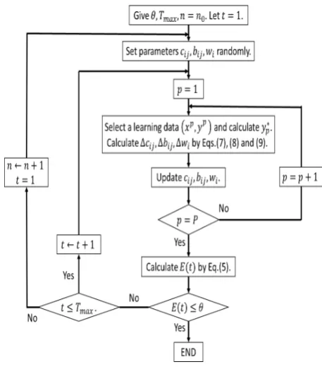
The conventional learning algorithm is shown as Fig.1 [1], [2], [11], where n0, θ and Tmax are the initial number
of rules, threshold and the maximum number of learning, respectively. Note that the method is generative one. The method is called learning algorithm A.
B. Neural gas and K-means methods
Vector quantization techniques encode a data space, e.g., a subspaceV⊆Rm, utilizing only a finite setC={c
i|i∈Zr} of reference vectors (also called cluster centers), where m andrare positive integers.
Let the winner vectorci(v)be defined for any vectorv∈V
as follows:
i(v) = arg min i∈Zr
||v−ci|| (10)
, where ||a−b|| means the distance between vectorsaand
b.
From the finite setC, V is partioned as follows:
Vi={v∈V|||v−ci||≤||v−cj|| f or j∈Zr} (11)
The evaluation function for the partition is defined as follows:
E= r ∑
i=1
∑
v∈Vi
[image:2.595.310.539.51.313.2]||v−ci(v)||2 (12)
Fig. 1. The flowchart of the conventional learning algorithm
For neural gas method [15], the following method is used: Given an input data vector v, we determine the neighborhood-rankingcik for k∈Zr∗−1, being the reference
vector for which there arek vectorscj with
||v−cj||<||v−cik|| (13)
If we denote the numberkassociated with each vectorci byki(v,ci), then the adaption step for adjusting theci’s is given by
△ci = ε·hλ(ki(v,c))·(v−ci) (14) hλ(ki(v,c)) = exp(−ki(v,c)/λ) (15)
where ε∈[0,1] and λ > 0. The number λ is called decay constant.
If λ→0, Eq.(14) becomes equivalent to the K-means method [15]. Otherwise, not only the winner ci0 but the second, third nearest reference vectorci1,ci2, etc., are also updated.
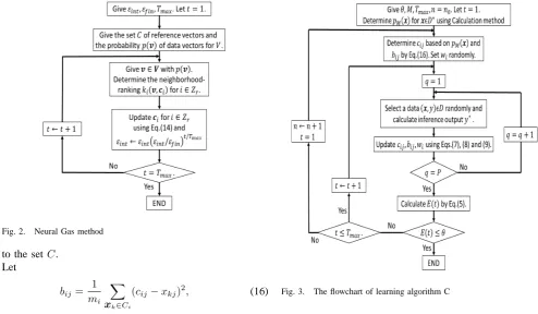
Letp(v)be the probability distribution of data vectors for V. The flowchart of the conventional neural gas algorithm is shown as Fig.2 [15], where εint, εf in, θ and Tmax are learning constants, threshold and the maximum number of learning, respectively. The method is called learning algo-rithm NG.
If the data distribution p(v) is not given in advance, a stochastic sequence of input data v(1),v(2),· · · which is based onp(v)is given [15].
By using Learning Algorithm NG, learning method of fuzzy systems is shown as follows [9], [10] : In this case, assume that the distribution of learning dataD∗ is discrete uniform one. Letn0 be the initial number of rules.
Learning Algorithm B
Step B1 : For learning dataD∗, Learning Algorithm NG is performed by usingD∗ as the setV. The setD∗ is encoded by the setC of reference vectors, where|C|=n0.
Fig. 2. Neural Gas method
to the setC. Let
bij= 1 mi
∑
xk∈Ci
(cij−xkj)2, (16)
whereCi andmi are thei-th cluster for C and the number of learning data fori∈Zn0. Each initial weightwi is selected randomly.
Step B3 : Learning algorithm A for initial parameters cij, bij andwi are performed.
C. The probability based on the rate of output change for learning data
Learning Algorithm B is a method that determines the initial assignment of fuzzy rules by vector quantization using the set D∗ of input for learning data. In this case, the set of output in learning data D is not used to determine the initial assignment of fuzzy rules. In the previous paper, we proposed a method considering both input and output data to determine the initial assignment of fuzzy rules [5].
Based on the literature [5], the probability distribution for D∗ is defined as follows : Let D and D∗ be the sets of learning data defined in 2.1.
Calculation of the probability for learning data
Step 1 : Give an input data xi∈D∗, we determine the neighborhood-ranking (xi0,xi1,· · ·,xik,· · ·,xiP−1) of the vector xi with xi0 = xi, xi1 being closest to xi and
xik(k= 0,· · ·, P −1) being the vector xi for which there
are kvectorsxj with||xi−xj||<||xi−xik||.
Step 2 : DetermineH(xi)which shows the rate of change of inclination of the output around output data to input data
xi, by the following equation:
H(xi) = M ∑
l=1
|yi−yil|
||xi−xil|| (17)
, where xil for l∈ZM means thel-th neighborhood-ranking
of xi, i∈ZP and yi and yil are output for input xi and xil, respectively. The numberM means the range of ranking
consideringH(x).
Step 3 : Determine the probability pM(xi) for xi∈D∗ by
Fig. 3. The flowchart of learning algorithm C
normalizingH(xi).
pM(xi) = H(x i) ∑P
j=1H(xj)
(18)
[image:3.595.45.540.53.341.2]and∑Pi=1pM(xi) = 1. [Example 1]
Let us explain how to compute pM(x) using y = sin(πx3
1)x2 as shown in Fig.4, where x1, x2, y∈[0,1].
Assume that four learning data are given as follows :
x y
x1= (0.2,0.2) 0.005
x2= (0.2,0.8) 0.020
x3= (0.8,0.2) 0.200
x4= (0.8,0.8) 0.799 LetM = 2.
Then,H(x1)is calculated as follows :
H(x1) = |y
1−y2|
||x1−x2||+
|y1−y3|
||x1−x3|| (19)
= 0.35
because the first and second closest vectors for x1 are x2
andx3.
Likewise, we obtained H(x2) = 1.325,H(x3) = 1.325
and H(x4) = 2.3. From the Eq.(18), each of p2(x)’s is
calculated as p2(x1) = 0.066, p2(x2) = 0.25, p2(x3) =
0.25,p2(x4) = 0.434.
IfM = 3, then the following result is obtained :
p3(x1) = 0.143,p3(x2) = 0.21,p3(x3) = 0.169,p3(x4) =
0.477.
In both cases, the rate of output change forx4= (0.8,0.8)
is large compared to other points, sopM(x4)is large.
The flowchart of learning algorithm C using pM(x) is shown in Fig.3 [5].
Fig. 4. The figure ofy=sin(πx3 1)x2
[Example 2]
Let us consider two cases with M = 1 and 100 using y = sin(πx3
1)x2, where Fig.5(a) and (b) are the initial
assignment of center parameters for four fuzzy rules using pM(x)withM = 1and100for the number of learning data P = 500, respectively. Fig.5(c) and (d) are the assignment of fuzzy rules after learning for M = 1 and100, respectively. The result shows that the case of M = 100 is superior in the assignment of fuzzy rules after learning to the case of M = 1. Please see Ref. [11] about the detailed explanation of Algorithm C.
It is known that many rules are needed at or near palaces where output changes quickly for learning data. The proba-bilitypM(x)is a technique to find the optimum places for the assignment of fuzzy rules. The algorithm C is a heuristic method to find the optimum number of M.
III. THE PROPOSED METHOD
It is shown that learning algorithms A, B and C using VQ and SDM is effective in accuracy and the number of rules to other methods. Most of conventional learning methods using VQ are ones that determine initial assignment of parameters in antecedent part for membership functions. However, little learning methods using VQ in learning process of SDM have been proposed.
The method using VQ in SDM means that each learning data in SDM is not selected randomly, but selected based on pM(x). Therefore, each data existing the place where output rapidly changes is more likely to be selected. Let explain it using Example 1.
[Example 3]
LetM = 2in Example 1. Thenp2(x1) = 0.066,p2(x2) =
0.25,p2(x3) = 0.25and p2(x4) = 0.434, so learning data
(x1, y1),(x2, y2),(x3, y3)and(x4, y4)∈Dare selected with the probability 0.066,0.25,0.25and0.434, respectively.
In this case, output change for (x4, y4) and(x1, y1) are
rapidly and flat as shown in Fig.4, respectively. It seems to assign a lot of fuzzy rules at or near the place(x4, y4).
In this section, we propose three algorithms usingpM(x) in learning steps of SDM corresponding to algorithms A, B and C. They are called algorithms(methods) A’, B’ and C’. The algorithm C’ is only shown as follows:
Learning Algorithm C’
Step 1 : θ,Tmax0 ,TmaxandM are set. Initial values ofcij, bij andwi are set randomly. n←n0.
Step 2 : Let t= 1.
Step 3 : Select a data(xp, yp)based onpM(xp)forp∈ZP.
Step 4 : Update cij by Eq.(14).
Step 12 : IfE < θ or t > Tmax go to Step 13, otherwise go to Step 8 witht←t+ 1, where E is computed as Eq.(5).
Step 13 : IfE < θthe algorithm terminate, otherwise go to Step 2 withn←n+ 1 andcij,bij andwi are set randomly.
The feature of the proposed method is that learning data are selected from the probabilitypM(x)in both determining of the initial assignment of parameters and learning steps of SDM(See steps 3 and 8 in learning algorithm C’).
In order to compare the proposed method with con-ventional ones, the following methods are introduced (See Fig.6):
(A) Method A is one based on the conventional algorithm of Fig.1 [1], [2]. Initial parameters of c, b and w are set randomly and all parameters are updated by SDM using learning data selected randomly until the inference error become sufficiently small.
(B) Method B is known as learning method of RBF networks [2], [3], [10]. Initial values ofcare determined usingD∗by VQ and b is computed using c. Weight parameters w are randomly selected. Further, all parameters are updated by SDM until the inference error become sufficiently small. (C) Method C was introduced in the chapter II. Initial values of c are determined using D by VQ and b is computed using c. Weight parameters are randomly selected. Further, all parameters are updated by SDM until the inference error become sufficiently small.
(A’) Method A’ is the proposed one. Initial parameters ofc,
b and w are set randomly and all parameters are updated using SDM using learning data based on pM(x) until the inference error become sufficiently small.
(B’) Method B’ is the proposed one. Initial values of c
are determined using D∗ by VQ and b is computed using
c. Weight parameters w are randomly selected. Further, all parameters are updated by SDM based on pM(x) until the inference error become sufficiently small.
(C’) Method C’ is the proposed one. Initial values of c
are determined using D by VQ and b is computed using
c. Weight parameters are randomly selected. Further, all parameters are updated by SDM based on pM(x) until the inference error become sufficiently small.
IV. NUMERICAL SIMULATIONS
In order to show the effectiveness of proposed algorithms, simulations of function approximation and classification problems are performed.
A. Function approximation
(a)The initial assignment of rules forM = 1
(c)The assignment of rules after learning forM = 1
[image:5.595.78.509.52.340.2](b)The initial assignment of rules forM = 100 (d)The assignment of rules after learning forM = 100 Fig. 5. The figures (a) and (b) show the initial assignment forM= 1and100, respectively, where◦and•mean the places of learning data and center parameters of fuzzy rules. The figures (c) and (d) show the assignment after learningM= 1and100, respectively.
Fig. 6. Concept of conventional and proposed methods, where SDM andd NG mean Steepest Descent Method and Neural Gas method. The algorithm C’ is only shown, and algorithms A’ and B’ are also defined in the same way.
(21)) and [−1,1]4((22) and (23)), and one output with the
range [0,1];
y = (2x1+ 4x
2 2+ 0.1)
2
37.21
×(4 sin(πx3) + 2 cos(πx4) + 6)
12 (20)
y = (sin(2πx1)×cos(x2)×sin(πx3)×x4+ 1.0) 2.0
(21)
y = (2x1+ 4x
2 2+ 0.1)2
74.42
TABLE I
THE RESULTS FOR FUNCTION APPROXIMATION
Eq(20) Eq(21) Eq(22) Eq(23) the number of rules 4.2 13.6 7.2 5.1 A MSE for Learning(×10−4) 0.40 0.71 0.43 0.28
MSE of Test(×10−4) 0.52 1.09 1.00 0.49
the number of rules 5.6 14.9 5.2 3.7 B MSE of Learning(×10−4) 0.18 0.77 0.49 0.33
MSE of Test(×10−4) 0.27 1.42 1.11 0.48
the number of rules 4.8 15.6 5.5 4.0 C MSE of Learning(×10−4) 0.21 0.72 0.54 0.88
MSE of Test(×10−4) 0.34 1.33 0.69 0.53 the number of rules 3.3 7.8 5.5 3.7 A’ MSE for Learning(×10−4) 0.22 0.63 0.43 0.27
MSE of Test(×10−4) 0.30 1.10 0.58 0.33 the number of rules 3.1 7.0 4.9 3.4 B’ MSE of Learning(×10−4) 0.21 0.66 0.57 0.25
MSE of Test(×10−4) 0.26 2.30 0.69 0.27
the number of rules 3.2 7.1 4.7 3.1 C’ MSE of Learning(×10−4) 0.21 0.65 0.60 0.22
MSE of Test(×10−4) 0.26 0.91 0.73 0.25
+(3e
3x3+ 2e−4x4)−0.5−0.077
4.68 (22)
y = (2x1+ 4x
2 2+ 0.1)2
74.42
+(4 sin(πx3) + 2 cos(πx4) + 6)
446.52 (23)
As the initial conditions of simulations, Tmax = 50000, Kc = 0.01, Kb = 0.01, Kc = 0.1, εinit = 0.1, εf in = 0.01, λ = 0.7, θ = 1.0×10⁻⁴ and M = 200 are used.
The numbers of learning and test data are 512 and 6400, respectively.
[image:5.595.356.490.64.174.2] [image:5.595.303.563.405.674.2]the number of rules 3.4 7.8 14.4 A RM for Learning(%) 3.0 1.4 1.6
RM of Test(%) 3.3 10.3 4.3 the number of rules 2.0 20.8 26.0 B RM of Learning(%) 3.3 13.6 2.2
RM of Test(%) 3.3 16.6 3.5 the number of rules 3.4 7.4 9.6 C RM of Learning(%) 2.8 2.1 2.0 RM of Test(%) 4.7 5.1 4.6 the number of rules 2.2 2.2 3.7 A’ RM for Learning(%) 2.7 1.5 1.5 RM of Test(%) 3.6 7.7 4.1 the number of rules 2.2 2.6 2.5 B’ RM of Learning(%) 2.4 1.3 1.7 RM of Test(%) 3.9 7.7 4.0 the number of rules 2.2 2.5 2.6 C’ RM of Learning(%) 2.4 1.4 1.6 RM of Test(%) 3.8 8.2 4.0
The result of simulation is the average value from twenty trials. As a result, proposed methods A’, B’ and C’ reduce the number of rules compared to conventional methods. Specifically, algorithm C’ is superior to other algorithms.
B. Classification problems for UCI database
Iris, Wine and BCW data from UCI database shown in Table II are used as the second numerical simulation [16]. In this simulation, 5-fold cross-validation is used. As the initial conditions for classification problem, Tmax= 50000,Kc= 0.001, Kb = 0.001, Kw = 0.05, εinit = 0.1, εf in = 0.01 andλ= 0.7are used. Further,M = 100andθ= 1.0×10⁻²
for Iris and Wine andM = 200andθ= 2.0×10⁻²for BCW
are used.
Table III shows the result of classification problem. In Table III, the number of rules, RM’s for learning and test data are shown, where RM means the rate of misclassification. As a result, it is shown that proposed methods A’, B’ and C’ reduce the number of rules in classification problem.
Let us consider the reason why we can get the good result by using the probability pM(x). In the conventional learning method, parameters are updated by any data selected randomly from the set of learning data. In the proposed method, parameters are updated by any data selected from the probabilitypM(x). The functionpM(x)is determined based on output change for the set of learning data, so many fuzzy rules are likely to generate at or near the places where output change is large for the set of learning data. For example, if the number of learning time is 100 andpM(x0) = 0.5, then
learning datax0is selected 50 times from the set of learning data in learning. As a result, membership functions are likely to generate at or near the places where output change is large for the set of learning data. The probability pM(x)is considered as a method to improve the local search of SDM.
numerical simulations for function approximation and pattern classification problems were performed. In the future work, we will propose more effective learning algorithm using the probability of output change for learning data compared to other methods and consider to apply the proposed method to learning of neural network.
REFERENCES
[1] B. Kosko, Neural Networks and Fuzzy Systems, A Dynamical Systems Approach to Machine Intelligence, Prentice Hall, Englewood Cliffs, NJ, 1992.
[2] M.M. Gupta, L. Jin and N. Homma, Static and Dynamic Neural Networks, IEEE Press, 2003.
[3] J. Casillas, O. Cordon, F. Herrera and L. Magdalena, Accuracy Improvements in Linguistic Fuzzy Modeling, Studies in Fuzziness and Soft Computing, Vol. 129, Springer, 2003.
[4] S. M. Zhoua and J. Q. Ganb, Low-level interpretability and high-level interpretability: a unified view of data-driven interpretable fuzzy system modeling, Fuzzy Sets and Systems 159, pp.3091-3131, 2008. [5] K. Kishida and H. Miyajima, A Learning Method of Fuzzy Inference Rules using Vector Quantization, Proc. of the Int. Conf. on Artificial Neural Networks, Vol.2, pp.827-832, 1998.
[6] O. Cordon, A historical review of evolutionary learning methods for Mamdani-type fuzzy rule-based systems, Designing interpretable genetic fuzzy systems, Journal of Approximate Reasoning, 52, pp.894-913, 2011.
[7] N. Yubazaki, J. Yi and K. Hirota, SIRMS(Single Input Rule Mod-ules) Connected Fuzzy Inference Model, J. Advanced Computational Intelligence, 1, 1, pp.23-30, 1997.
[8] H. Miyajima, N. Shigei and H. Miyajima, Fuzzy Inference Systems Composed of Double-Input Rule Modules for Obstacle Avoidance Problems, IAENG International Hournal of Computer Science, Vol. 41, Issue 4, pp.222-230, 2014.
[9] K. Kishida, H. Miya jima, M. Maeda and S. Murashima, A Self-tuning Method of Fuzzy Modeling using Vector Quantization, Proceedings of FUZZ-IEEE’97, pp397-402, 1997.
[10] S. Fukumoto, H. Miyajima, N. Shigei and K. Uchikoba, A Decision Procedure of the Initial Values of Fuzzy Inference System Using Counterpropagation Networks, Journal of Signal Processing, Vol.9, No.4, pp.335-342, 2005.
[11] H. Miyajima, N. Shigei, K. Kishida, Y. Akiyoshi and H. Miyajima, An Improved Learning Algorithm of Fuzzy Inference Systems using Vector Quantization, Advanced in Fuzzy Sets and Systems, Vol.20, pp.155-175, 2015.
[12] H. Miyajima, N. Shigei, H. Miyajima, Fast Learning Algorithm for Fuzzy Inference Systems Using Vector Quantization, Int. MultiConfer-ence of Engineers and Computer Scientists 2016, Vol.I, pp.1-6, Hong Kong, March, 2016.
[13] H. Miyajima, N. Shigei and H. Miyajima, The Ability of Learning Algorithms for Fuzzy Inference Systems using Vector Quantization, ICONIP 2016, LNCS 9950, pp.479, Kyoto, October, 2016.
[14] W. Pedrycz, H. Izakian, Cluster-Centric Fuzzy Modeling, IEEE Trans. on Fuzzy Systems, Vol. 22, Issue 6, pp. 1585-1597, 2014.
[15] T. M. Martinetz, S. G. Berkovich and K. J. Schulten, Neural Gas Network for Vector Quantization and its Application to Time-series Prediction, IEEE Trans. Neural Network, 4, 4, pp.558-569, 1993. [16] UCI Repository of Machine Learning Databases and Domain Theories,