A Dual Extended Kalman Filter for Tilt Estimation

A Dual Extended Kalman Filter for Tilt

Estimation

Herman I. Veriñaz, Edgar M. Vela,

Member, IAENG,

Ronald A. Ponguillo,

Member, IAENG

Abstract— Accelerometers and Gyroscopes are typically used to measure rotation angles. However, the nature of both sensors makes difficult to estimate an angle using only one of these sensors. This is because gyroscopes return high bias data, and, since accelerometers detects every small acceleration in each axis, the output of this sensor is very noisy.

A common solution is to combine both signals in so-called sensor fusion. Two popular techniques are Complementary Filters and Constant Gyro Bias Kalman Filters. These algorithms are attractive because they are simple to implement and do not depend on specific parameters of the system.

Because these filters use the arctangent function, they cannot resolve a discontinuity on the estimated signal. This discontinuity is caused by a flip among the two endpoints in the range of arctangent function. This range is usually [-π/2, π/2] or [-π, π]. This problem occurs because of the discontinuous nature of the tangent function, and because tangent is strictly not invertible. To solve this, an additional routine must be implemented to patch these flips.

This paper presents a practical Dual Extended Kalman Filter algorithm for angle estimation. This work focus on the restricted problem of measuring the angle of rotation of a body respect to one axis parallel to the earth surface. The main characteristic of the developed algorithm is that it does not depend on physical parameters and does not use the inverse tangent function on its implementation.

For the implementation, the accelerometer and gyro signals were acquired from the IMU MPU-6050 with a 50 ms sampling time. The complete algorithm was implemented in a MATLAB script and then it was compared with two other methods usually used in tilt estimation: Complementary Filters and Constant Gyro Bias Kalman Filter.

Index Terms—Angle Estimation, Dual Extended Kalman Filter, Sensor Fusion, Kalman Filter, Tilt Estimation.

I. INTRODUCTION

n many applications it is needed to know the orientation of a body respect to a certain coordinate system. This work Manuscript received March 20, 2017; revised March 28, 2017.

H. I. Veriñaz is with the Escuela Superior Politécnica del Litoral, ESPOL, Faculty of Natural Science and Mathematics, Campus Gustavo Galindo, Km 30.5 Via Perimetral, P.O. Box 09-01-5863, Guayaquil, Ecuador (e-mail: [email protected]).

E. M. Vela is an engineer in Electronics and Telecommunications, graduated at Escuela Superior Politécnica del Litoral, ESPOL, Faculty of Electrical and Computer Engineering, Campus Gustavo Galindo, Km 30.5 Via Perimetral, P.O. Box 09-01-5863, Guayaquil, Ecuador (e-mail: [email protected]).

R. A. Ponguillo is the Coordinator of the Basic Electronics Area and a Researcher of the Vision and Robotics Center at the Escuela Superior Politécnica del Litoral, ESPOL, Faculty of Electrical and Computer Engineering, Campus Gustavo Galindo, Km 30.5 Via Perimetral, P.O. Box 09-01-5863, Guayaquil, Ecuador (e-mail: [email protected]).

focus on the restricted problem of measuring the angle of rotation of a body respect to one axis parallel to the earth surface.

There are two common sensors used to measure this orientation: accelerometers, and gyroscopes. One way of doing this is to use an accelerometer to find the gravity components, then the angle is calculated using an inverse tangent function. Other form is to use a gyroscope to measure the angular speed, and the angle is simply this angular speed accumulated over the time.

Both techniques have their drawbacks. The accelerometer does not measure only the gravity components. It also measures every small acceleration in each axis, so its signals are usually noisy. On the other hand, the gyroscope is less noisy but the accumulation of the angular speed over the time also causes an accumulation of the noise, producing a bias in the angle signal.

To overcome these problems two popular techniques of sensor fusion are usually used: Complementary filters and Kalman filters [2] [4].

A complementary filter is employed because it is very practical, and has low computational complexity. It is a weighted sum of the gyro and accelerometer data:

𝜃𝑘+1 = 𝑎(𝜃𝑘+ 𝜔𝑘) + (1 − 𝑎)𝑧𝑘 (1)

𝑧𝑘 = arctan⁡(𝑎_{𝑚𝑡 𝑘}/𝑎_{𝑚𝑟 𝑘})

𝑎: Adjustable parameter between 0 and 1. 𝑧𝑘: Measured angle at the kth instant.

𝑎_{𝑚𝑡 𝑘}

:

Measured tangential acceleration at the kth instant.

𝑎_{𝑚𝑟 𝑘}

:

Measured radial acceleration at the kth instant.

𝜃𝑘

:

Angle of rotation at the kth instant.

𝜔

𝑘

:

Angular velocity at the kth instant.

Also, it is typically preferred a Linear Kalman filter [2] using the following constant gyro bias model:

𝜃𝑘+1 = 𝜃𝑘+ (𝑏𝑘+ 𝜔𝑘) (2)

𝑏𝑘+1= 𝑏𝑘

𝑏𝑘: Gyroscope bias at the kth instant.

Both filters are simple to implement and do not depend on physical parameters.

physical parameters, does not use the arctangent function and it was designed and tested using MATLAB software.

II. MATHEMATICAL MODEL

As mentioned in the introduction, this model greatly relies on the angular speed measured with the gyroscope. Ideally, the measured angle is simply the accumulated angular speed over the time. If the sampling time is one, the equation is:

𝜃𝑘+1= 𝜃𝑘

+ 𝜔

𝑘

(3)

𝜃𝑘

:

Measured angle at the kth instant.

𝜔

𝑘

:

Angular velocity at the kth instant.

To improve the model, additional information is obtained from the accelerometer. The accelerometer measures the gravity and the acceleration at the same time. This is represented as:

𝑎_𝑚𝑡𝑘= 𝑎_𝑡𝑘+ 𝑔𝑐𝑜𝑠(𝜃𝑘) (4)

𝑎_{𝑚𝑟 𝑘}= 𝑎_{𝑟 𝑘}+ 𝑔𝑠𝑖𝑛(𝜃𝑘)

𝑎_𝑡𝑘

:

Tangential acceleration at the kth instant.

𝑎_𝑟𝑘

:

Radial acceleration at the kth instant.

𝑎_𝑚𝑡𝑘

:

Measured tangential acceleration at the kth instant.

𝑎_{𝑚𝑟 𝑘}

:

Measured radial acceleration at the kth instant.

𝑔

:

Local gravity.

The tangential and radial acceleration are:

𝑎_𝑡𝑘 = 𝑟𝛼𝑘+ 𝑎𝑡𝑘𝑐𝑚 (5) 𝑎_{𝑚𝑟 𝑘}= −𝑟𝜔𝑘2+ 𝑎𝑟𝑘_𝑐𝑚 (6)

𝛼

𝑘

:

Angular acceleration respect to the center of curvature at the kth instant.

𝑟

:

Radius of curvature.

𝑎𝑡𝑘𝑐𝑚

:

Tangential acceleration of the center of mass

relative to an inertial frame.

𝑎𝑟𝑘𝑐𝑚

:

Radial acceleration of the center of mass relative to

an inertial frame.

The terms 𝑎𝑡𝑘_𝑐𝑚 and 𝑎𝑟𝑘_𝑐𝑚 can be used to give additional information to the system. For example, if it is plausible, an additional accelerometer can be placed in the center of mass. On this work,a null acceleration model is used for the center of mass. Thus, the center of mass is the inertial frame.

The radius of curvature is a parameter needed for the implementation. In specific applications, this parameter can be measured directly, but for generality and practicability of the filter, it is assumed unknown. As there is not much information about this parameter, therefore a simple model is used:

𝑟𝑘+1= 𝑟𝑘 (7)

Even though the radius is assumed to be constant, the appropriate tuning of the Kalman filter will allow this estimated value to change over the time.

Thus, the complete model is:

𝜃𝑘+1 = 𝜃𝑘

+ 𝜔

𝑘

(8)

𝑟𝑘+1= 𝑟𝑘

𝑧𝑘

= ℎ(

𝑟𝑘, 𝜃𝑘

, 𝛼

𝑘

, 𝜔

𝑘

) =

(

𝑟𝑘

𝛼

𝑘

+ 𝑔𝑐𝑜𝑠(

𝜃𝑘

)

−

𝑟𝑘

𝜔

𝑘2

+ 𝑔𝑠𝑖𝑛(

𝜃𝑘

)

)

𝛼

𝑘

:

Angular acceleration at the kth instant.

𝑟𝑘

:

Radius of curvature.

𝑔

:

Local gravity.

𝜃𝑘

:

Angle of rotation at the kth instant.

𝜔

𝑘

:

Angular velocity at the kth instant.

𝑧𝑘: Observation vector

III. Kalman Filter

The algorithm for the implementation is a Dual Extended Kalman Filter [1] (DEKF). A linear Kalman filter [2] and an extended Kalman filter are executed at the same time, for the radius estimation and angle estimation respectively. The Kalman equations are:

Prediction:

𝜃̂𝑘|𝑘−1= 𝜃̂𝑘−1|𝑘−1

+ 𝜔

𝑘

(9)

𝑃_{𝜃 𝑘|𝑘−1}= 𝑃_{𝜃 𝑘−1|𝑘−1}

+

𝑄_{𝜃 𝑘}

𝑟̂𝑘|𝑘−1= 𝑟̂𝑘−1|𝑘−1

𝑃_{𝑟 𝑘|𝑘−1}= 𝑃_{𝑟 𝑘−1|𝑘−1}

+

𝑄_𝑟⁡𝑘

Update:

𝑌𝑘 = 𝑧𝑘−

ℎ

(𝑟̂𝑘|𝑘−1, 𝜃̂𝑘|𝑘−1

, 𝛼

𝑘

, 𝜔

𝑘) (10) 𝐾_{𝜃 𝑘}= 𝑃_{𝜃𝑘|𝑘−1}𝐻_𝜃𝑘𝑇(𝐻_{𝜃 𝑘}𝑃_{𝜃𝑘|𝑘−1}𝐻_𝜃𝑘𝑇+ 𝑅𝑘)

−1

(11)

𝜃̂

𝑘|𝑘

= 𝜃̂

𝑘|𝑘−1

+ 𝐾

𝑘

𝑌

𝑘

(12)

𝑃_{𝜃 𝑘|𝑘}= (𝐼 − 𝐾_{𝜃 𝑘}𝐻_{𝜃 𝑘})𝑃_{𝜃 𝑘|𝑘−1} (13)

𝐾_{𝑟 𝑘}= 𝑃_{𝑟𝑘|𝑘−1}

𝐻

_𝑟𝑘𝑇(

𝐻

_𝑟𝑘𝑃_{𝑟𝑘|𝑘−1}

𝐻

_𝑟𝑘𝑇

+ 𝑅

𝑘) −1

(14) 𝑟̂𝑘|𝑘 = 𝑟̂𝑘|𝑘−1

+

𝐾𝑘𝑌𝑘 (15)

𝑃𝜃𝑘|𝑘 = (𝐼 − 𝐾𝑟𝑘

𝐻

𝑟𝑘)𝑃𝑟𝑘|𝑘−1 (16)

The observation model matrix H, for each state variable is the gradient of

ℎ,

which is the observation model function

.

𝐻

_𝑟𝑘=

(

−𝜔

𝛼

𝑘

𝑘2

)

For the angle, the gradient matrix is:

𝐻

_𝜃𝑘=

(

−𝑔𝑠𝑖𝑛(𝜃

̂

𝑘|𝑘−1)

𝑔𝑐𝑜𝑠(𝜃

̂

𝑘|𝑘−1)

)

The vector 𝑧𝑘 is the pair of measured accelerations:

𝑧𝑘 = (

𝑎_{𝑚𝑡 𝑘} 𝑎_{𝑚𝑟 𝑘})

Finally, notice that matrix

𝑅

_𝑘is symmetric because signals are real, and Q matrices are simply real numbers:

𝑅

𝑘⁡ ∈ 𝑆2𝑥2

These equations can be implemented in an IDE that handle matrices, like MATLAB. However, the idea is to obtain one-dimensional equations that could be easily implemented in a microcontroller. To simplify the problem, it was assumed that the observation noise is uncorrelated. This means the matrix

𝑅

𝑘is diagonal.

Notice that the prediction equations (9) are one-dimensional equations and (10) can be write as two simple one-dimensional equations.

Now, to compute the gain matrix 𝐾_{𝜃 𝑘} it is needed to calculate a determinant result of the inverse in equation (11), the equation is:

(17)

𝑑𝑒𝑡𝜃= 𝑔2𝑝𝜃𝑘|𝑘−1((𝑟11− 𝑟22) 𝑐𝑜𝑠2⁡(𝜃̂𝑘|𝑘−1) + 𝑟22) + 𝑟11𝑟22

Then, the two components of the matrix 𝐾_{𝜃 𝑘}can be obtained using equation (11), these are:

𝐾_𝜃1𝑘= −𝑔𝑝𝜃𝑘|𝑘−1𝑠𝑖𝑛(𝜃_𝑑𝑒𝑡̂𝑘|𝑘−1)𝑟22

𝜃 (18)

𝐾_𝜃2𝑘=𝑔𝑝𝜃𝑘|𝑘−1𝑐𝑜𝑠(𝜃_𝑑𝑒𝑡̂𝑘|𝑘−1)𝑟11

𝜃 (19)

To compute the equations (12) and (13) it is needed to do some matrix algebra, the reduced expressions are:

𝜃̂𝑘|𝑘= 𝜃̂𝑘|𝑘−1+ 𝐾𝜃1𝑘𝑌𝑘1+ 𝐾𝜃2𝑘𝑌𝑘2 (20)

𝑝_{𝜃𝑘|𝑘}= 𝑝_{𝜃𝑘|𝑘−1}(𝑔𝐾_𝜃1𝑘𝑠𝑖𝑛(𝜃𝑘) ⁡ − 𝑔𝐾𝜃2𝑘𝑐𝑜𝑠(𝜃𝑘) ⁡⁡ + ⁡1) (21)

In the same way, the equations for the radius are:

𝑑𝑒𝑡𝑟= 𝑝𝑟 𝑘|𝑘−1𝑟11𝜔𝑘4+ 𝑝𝑟 𝑘|𝑘−1𝑟22𝛼𝑘2⁡ + ⁡ 𝑟11𝑟22 (22)

𝐾_𝑟1𝑘=𝛼𝑘𝑝𝑟𝑘|𝑘−1𝑟22

𝑑𝑒𝑡𝑟 (23)

𝐾_{𝑟 2𝑘}= −𝜔𝑘

2_𝑝 𝑟𝑘|𝑘−1𝑟11

𝑑𝑒𝑡𝑟 (24)

𝑟̂𝑘|𝑘= 𝑟̂𝑘|𝑘−1+ 𝐾𝑟1𝑘𝑌𝑘1+ 𝐾𝑟 2𝑘𝑌𝑘2 (25)

𝑝_{𝑟 𝑘|𝑘}= 𝑝_{𝑟 𝑘|𝑘−1}(−𝐾_𝑟1𝑘𝛼𝑘+ 𝐾𝑟 2𝑘𝜔𝑘2⁡⁡+ ⁡1) (26)

Once these equations are obtained, it is needed to define the values of the covariance matrices

𝑅

𝑘

,

𝑄𝜃 𝑘and 𝑄𝑟⁡𝑘.There is no standard method to obtain these matrices. On this implementation, they were tuned manually by trial and error.

IV. IMPLEMENTATION AND RESULTS

For implementation, the MPU-6050 [3] was employed. This is a popular device among hobbyist. It is a MEMS accelerometer and a MEMS gyro in a single chip. For this implementation, both sensors were sampled each 50 ms.

The algorithm was tested using a MATLAB script. The equations implemented were the one-dimensional prediction equations (9), equation (10) and (17) to (26). Matrices Q and R obtained after the tuning are:

𝑅𝑘= (250_{0 250}0 )

[image:3.595.304.535.68.149.2] [image:3.595.62.550.342.601.2]

𝑄_𝜃𝑘= 0.000021 𝑄_𝑟⁡𝑘= 20

[image:4.595.59.539.48.663.2]

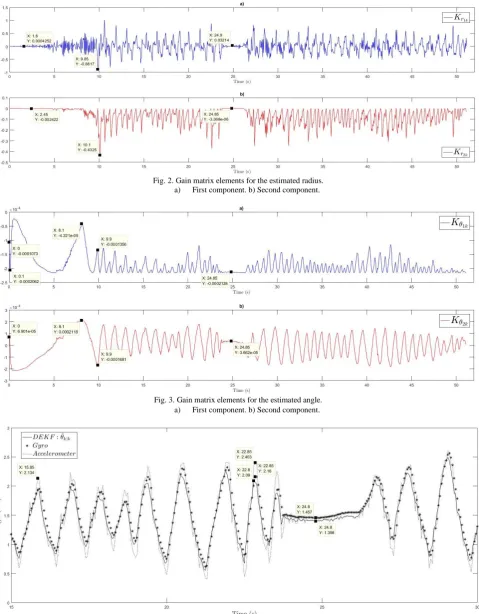
Fig. 2. Gain matrix elements for the estimated radius. a) First component. b) Second component.

Fig. 3. Gain matrix elements for the estimated angle. a) First component. b) Second component.

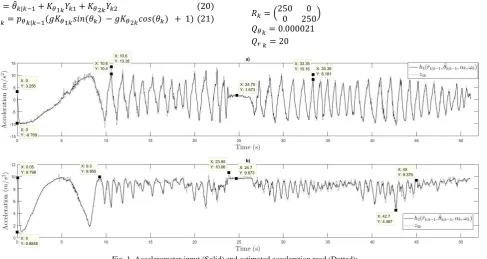
Fig. 4. Tilt angle measure using directly the Gyroscope reading, the Accelerometer reading, and the estimation using DEKF

An adequate tuning allows the predicted signals to follow the sensor signal. This is shown in Figure 1. The estimated signal does not have the same initial value than the read signals, but after approximately 0.5 seconds the filter converges, and both signals are approximately equal.

Notice, that while the filter output converged after 0.5 seconds, the gain matrices did not converge. The gain matrix

𝐾_{𝑟 𝑘}for the radius is shown in the Figure 2, and the gain matrix 𝐾_{𝜃 𝑘} for the angle is shown in the Figure 3. The elements of these matrices do not converge to any value, rather they are always being self-adjusted during the whole simulation.

signal, and with the angle calculated with the data acquired from the accelerometer.

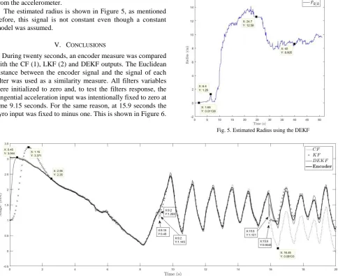
The estimated radius is shown in Figure 5, as mentioned before, this signal is not constant even though a constant model was assumed.

V. CONCLUSIONS

During twenty seconds, an encoder measure was compared with the CF (1), LKF (2) and DEKF outputs. The Euclidean distance between the encoder signal and the signal of each filter was used as a similarity measure. All filters variables were initialized to zero and, to test the filters response, the tangential acceleration input was intentionally fixed to zero at time 9.15 seconds. For the same reason, at 15.9 seconds the gyro input was fixed to minus one. This is shown in Figure 6.

[image:5.595.53.538.62.457.2]

Fig. 5. Estimated Radius using the DEKF

Fig. 6. Encoder measured angle compared with three filters: Complementary, Linear Kalman, and Dual Extended Kalman

The CF (1) was tune with a=0.8. This filter is the more distant to the encoder angle signal (d=20.0594 radians), but it is simpler to implement. Moreover, because it uses directly a weighted average between the gyro and accelerometer signals, the time of convergence is zero. For the same reason, at time 15.9 s the complementary filter cannot restore its estimated signal, but at time 9.15 s it was successfully restored.

The LKF model (2) is simpler than the DEKF, but its time of response is longer. This filter can successfully restore its value at 9.15 s and 15.9 s, and it has a distance to the encoder signal of d= 6.8386 radians. Nevertheless, when distances were measured between 9.85 and 14.65 seconds, these values were d=0.6047 radians, d=0.5105 radians and d=0.4805 radians, for the CF, LKF, DEKF respectively. It means that, if there is no perturbation, and all the filters have converged, the LKF estimation is closer to the encoder reading than the DEKF estimation.

The distance between the encoder signal and the DEKF signal is d=3.2505 radians, the shortest one. This is because this filter converges faster than the LKF and it has a better response to input perturbations, as shown in Figure 6.

The CF and the LKF stand out because of the simplicity of the model. However, it is important to note that, to estimate

angles out of the range of the arctangent function, it is needed to implement an additional routine to make the tangent continuous in the desired interval. The DEKF algorithm use directly the sine and cosine functions, so it does not need any additional routine.

REFERENCES

[1] Nejad, S. and Gladwin, D.T. and Stone, D.A., "On-chip implementation of Extended Kalman Filter for adaptive battery states monitoring," IECON Proceedings (Industrial Electronics Conference) 2016, pp. 5513-5518

[2] Jadan, H.I.V. and Vera, C.R.M. and Intriago, R.P. and Padilla, V.S., "Implementing a Kalman filter on FPGA embedded processor for speed control of a DC motor using low resolution incremental encoders," Lecture Notes in Engineering and Computer Science: Proceedings of World Congress on Engineering and Computer Science, WCECS 2016, Vol.1, pp.367-371

[3] InvenSense, "MPU-6000 and MPU-6050 Product Specification Revision 3.4", MPU600 Datasheet, Nov. 2010 [Revised Aug. 2013]