Particle / Kalman Filter for Efficient Robot Localization

(1)

Particle/Kalman Filter for Efficient Robot Localization

Imbaby I. Mahmoud

Nuclear Research Center Atomic Energy Authority

May Salama

Benha University, Faculty of Eng Computer Engineering. Dept

Asmaa Abd El Tawab

Nuclear Research Center, Atomic Energy Authority

ABSTRACT

This paper presents a comparison of different fitters namely: Extended Kalman Filter (EKF), Particle Filter (PF) and a proposed Enhanced Particle / Kalman Filter (EPKF) used in robot localization. These filters are implemented in matlab environment and their performances are evaluated in terms of computational time and error from ground truth and the results are reported. The considered robot localizer uses radio beacons that provide the ability to measure range only. Since EKF and its variants are not capable to efficiently solve the global localization problem, we propose the Enhanced Particle / Kalman Filter (EPKF) which provide the required initial location to address this drawback of EKF. We propose using PF as Initialization phase to coarsely predict the initial location and numerous sets of data are experimented to get robust conclusion. The results showed that the proposed localization approach which adopts the particle filter as initialization step to EKF achieves higher accuracy localization while, the computational cost is kept almost as EKF alone.

General Terms

Algorithms and robotics

Keywords

Particle Filter, Extended Kalman Filter, Robot Localization

1. INTRODUCTION

The problem of robot localization is known as answering the question Where am I or determining the place of the robot. This means that the robot is trying to locate it in comparison to the surrounding environment. When we research for location, pose, or position we mean the x and y coordinates and heading direction of a robot in a global coordinate system. The mobile robot localization problem comes in many multiple flavors. Position tracking is the simplest localization problem where the initial robot pose is known and the problem is to compensate incremental errors in a robot’s odometry. Global localization problem [1] is another challenging one, where a robot is not told its initial pose but instead has to determine it from scratch.

Several methods to support the robot localization problem showed in [2.3]. The Kalman filter applied often to the problem of localization of the robot. It works frequently, and it does not require a history of previous states of the robot. This results in a simplified algorithm that can run on the online in real-time systems. Unfortunately, the absolute rang measurements is a set of nonlinear (as in our case), which require the use of the Kalman Filter Extended (EKF), which must be linearized the measurements around the current state estimate. These results in a weakness common to all linear methods which means that the kalman filter will not converge when the initial state is not sufficiently accurate [4]

Recently Particle Filter (PF) becomes public approach used for treatment of this problem. This is due to its ability to deal with the problem of non-linear non-Gaussian problem, typical

features of the problem of localization [5.6] this. Several applications of PF in [7-9].In this paper, the particle filter is introduced to initialize kalman filter to overcome the initial state problem of original kalman filter. Different filters namely Kalman filter (KF), Particle Filter (PF) and a proposed Enhanced Particle/Kalman Filter (EPKF) implemented in Matlab environment and their performance are evaluated in terms of computational complexity and amount of error from ground truth .The obtained results are reported and compared. This paper is organized as follows: section 2 presents overview of an Enhanced Particle/Kalman filter and their implementation algorithms, section 3 studied the effect in Robot Localization by using different filters, section 4 shows the discussion of the obtained results,and finally section 5 is devoted to conclusion.

2. OVERVIEW OF AN ENHANCED

PARTICLE / KALMAN FILTER

The used absolute range measurements are non-linear, requiring the use of an Extended Kalman Filter (EKF), The kalman filter there is modified to filter known as extended kalman filter.

2.1 Extended Kalman Filter (EKF) for

Localization

[1] The motion model [10]

If the robot pose (position and heading) at time k is represented by the state vector

q

_k





x

_k

,

y

_k

,



_k



T then the motion model of the wheeled robot used in this experiment are completely-modeled by the following non-linear equations:

 

k

k k

k k k

k

y

D

v

D

X

q

































sin

cos

1

(1)

Where: vk is a noise vector. Here, ΔDk point at the center of the robot’s front axle, obtained by averaging the distances measured by the left and right wheel encoders. The incremental orientation change Δθk is obtained by the onboard gyro. These dead reckoning measurements forming the control input vector

u

_k







D

_k

,





_k



T

The system matrix A (k) is represented by the Jacobian:





 

























_

1

0

1 cos

1

0 sin

0

1 |

1

_ˆ _k _k

k k

q q k

D

q

f

k

A

k



(2)

The input gain matrix B(k) is was built similarly:

 

               _ 1 0 0 0 sin cos | ) 1

( _ˆ _k

k q q k k q f k B



(3)

[2] The measurement model [10]:

At time k+1 the range from a beacon located at (xb, yb) to the robot with state vector q k+1 can be written as:

 







 



2

1 2 1 ,

,

1 k b k b

T b b

k

x

y

x

y

q

h

_



_





_



(4)

[3] Time Propagation [11]

When a new control input vector

u

 

k







D

_k_,





_k



is received, the robot’s state is updated according to the process model equation. Using the standard equations of kalman filtering, the covariance matrix maintaining our uncertainty about the current state is propagated in time:

 

k

p

A

 

k

B

   

k

B

k

Q

 

k

A

p

_k



_k_₁ T





T



(5)

So, the state maintained during the time propagation step indicates the pose of the robot at the robot reference point. [4] The measurement update: [12]

When a measurement is obtained, using the method of the update step is broken up as follows:

* Shift the robot reference point’s coordinates to get the coordinates of the current antenna, (xa, ya)).

*Expecting the current measurement onto the xy plane of the robot.

* Using (xa, ya) and the known beacon location (xb, yb), compute Hk.

* Find the variance k R and the mean k y associated with the

current measurement from its previous stored PDF.

* Using the measurement model, compute the expected range rk to the beacon. Let υ (k) = y − r be the innovation.

* Compute

S

_k



H

_k

p

_k

H

_kT



R

_k

* Compute the Kalman gain

K

_k



p

_k

H

T_k

S

_k1_k

* Compute the normalized innovation squared and tests the measurement against the chi square

* If the measurement passes the gating test, update the state by letting

q

ˆ

_k



q

ˆ

_k



K

_k

v

 

k

and update the covariance matrix by letting

p

_k



p

_k



K

_k

S

_k

K

_kT.

* Now, employ this updated estimate of the pose at the antenna which reported the current measurement, shift back in x and y to get the updated pose estimate at the robot reference point.

2.2 Particle Filter Algorithm

The PFs are formulated on the concepts of the Bayesian theory and the sequential importance-sampling which are very effective in dealing with non-Gaussian and non-linear problems [13-16]

The PF approximates recursively the posterior distribution using a finite set of weighted samples. The idea is to represent the required posterior density function by a set of random samples with associated weights and to compute estimates based on these samples and weights. PF uses the probabilistic system transition model p (Xt|Xt-1), (which describes the

transition for state vector Xt) to predict the posterior at time t

as:

dX

)

Z

|

p(X

)

X

|

p(X

)

Z

|

p(X

_t ₁_:_t_-₁





_t _t_-₁ _t_-₁ ₁_:_t_-₁ _t_-₁ (6)

Where Z1: t-1 = {Z1, Z2,.... Zt-1} are available

observations at times 1, 2, …., t-1, p(Xt|Xt-1) expresses the

motion model, p(Xt-1|Z1: t-1) is posterior probability density

function at time t-1 and p(Xt|Z1: t-1) is the prior Probability

Density Function (PDF) at time t. At time t, the observation Zt

is available, then the state can be updated using Bayes's rule as:

)

Z

|

p(Z

)

Z

|

p(X

)

X

|

p(Z

)

Z

|

p(X

1 -t : 1 t 1 -t : 1 t t t t : 1

t



(7)

Where p(Zt|Xt) is described by the observation equation. The

posterior PDF p(Xt-1|Zt-1) is approximated recursively as a set

of N weighted samples





N

1 s

)

s

(

1 t

)

s

(

1 t

,

W

X

_

_

, and

)

s

(

1 t

W

_

is the weight for particle

(

s

)

1 t

X

_

. Using a Monte Carlo approximation of the integral, we get:

p (Xt|Zt) =p (Zt|Xt)



  N s s t

W

1 ) (

1 p (

) (

1

|

_ts

t

X

_ ) (8)

The N samples

X

_t(s)are drawn from the proposal distribution:

q(X) =



  N s s t

W

1 ) (

1 p (Xt|

)

s

(

1 t

X

_

) (9)

Then it is weighted by the likelihood.

) (s t

W

= p (Zt|

) s ( t

X

) (10) This produces a weighted particle approximation





N

s s t s

t

W

X

(_₁)

,

(_₁) _₁ for the posterior PDF p (Xt|Z t) at time t.

3. IMPLEMENTATION AND RESULTS

OF

ROBOT

LOCALIZATION

ALGORITHM

USING

STUDIED

FILTERS

(3)

repeating path. All studied filters approaches are used to fuse range data with dead reckoning data collected from a real system which integrates proprioceptive measurements from wheel encoders, gyros, and accelerometers to localize the robot. Mat lab environment is used for experimenting with localization process.

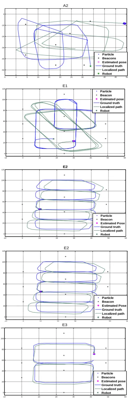
[image:3.595.316.532.68.746.2]

Fig [1] shows the dead reckoning path, ground truth path and tag locations for all paths dataset [A1, A2, E1, E2, E4, B1, and B2] from reference [18].Therefore different filters approaches [17-19] are introduced to improve this performance.

Fig .1: The ground truth path, tag locations and dead reckoning of B2 datastet.

We notice from these figures that the dead reckoning tends to move away from the true path with the passage of time. This is due to increasing errors in odometry. This can be a good localization method for a short distance, but it provides no means of recovering from error that accumulates in nature.

3.1 The Results Of The Different

Approaches

In this paper we have used numerous carefully-collected datasets and processed them with an extended kalman filter, a particle filter, and enhanced particle / kalman filter. Our implementation of particle filter in matlab environment requires no initial estimate of the robot’s position. In all experiments, the robot’s travel is clipped from results plot, giving the filter time to converge. Figs (2-4) show the results of studied filters. Table [1-7] summarizes the results of these figures concerning the error in the estimates of the studied filters.

-5 0 5 10 15 20 25 30 35 -35

-30 -25 -20 -15 -10 -5 0 5

A1

Particle Beacon Estimated pose Ground truth Localized path Robot

-5 0 5 10 15 20 25 30 35 40 45 50 -50

-40 -30 -20 -10 0

A2

Particle Beacons Estimated pose Ground truth Localized path Robot

-10 0 10 20 30 40 50 60 0

20 40 60 80 100

120 E1

-10 0 10 20 30 40 50 60 0

20 40 60 80 100 120

E2

Particle Beacon Estimated Pose Ground truth Localized path Robot

-10 0 10 20 30 40 50 60 0

20 40 60 80 100 120

E2

Particle Beacon Estimated Pose Ground truth Localized path Robot

-10 0 10 20 30 40 50 60 0

20 40 60 80 100 120

E3

[image:3.595.58.269.583.711.2]

(4)

Fig.2: Particle filters localization performance on all datasets

Fig.3: Extended kalman filter localization performance on all datasets

-10 0 10 20 30 40 50 0

20 40 60 80 100 120

B1

-10 0 10 20 30 40 50 -10

0 10 20 30 40

50 B2

-15 -10 -5 0 5 10 15 20 25 30 35 -35

-30 -25 -20 -15 -10 -5 0

A1

Beacon Ground T ruth Localized path Estimated Pose Robot

-20 -10 0 10 20 30 40 50 -50

-40 -30 -20 -10 0

A2

Beacon Ground truth Localized path Estimated pose Robot

-50 0 50 100

0 20 40 60 80 100

E1

-50 0 50 100

0 20 40 60 80 100

E2

Beacon Ground truth Localized path Estimated Pose Robot

-50 0 50 100

0 20 40 60 80 100

E3

Beacon ground truth Localizes path Estimated pose Robot

-50 0 50 100

0 20 40 60 80 100

B1

-20 -10 0 10 20 30 40 50 60 70 -10

0 10 20 30 40 50 60

B2

-15 -10 -5 0 5 10 15 20 25 30 35 -35

-30 -25 -20 -15 -10 -5 0

A1 Beacon

Initial pose of (KF) GT

Localized path Estimated pose Robot Robot Particle

(5)

[image:5.595.325.538.73.224.2]

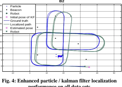
Fig. 4: Enhanced particle / kalman filter localization performance on all data sets

Table 1: Results of Error Calculation Using Different Filters in the Dataset (A1)

Error/in meter PF EKF EPKF

XTE_abs_avg 3.5883 0.8787 0.8841

XTE_abs_max 23.4162 2.5697 2.5673

XTE_abs_std 3.622 0.5946 0.5983

ATE_abs_avg 5.3397 1.1241 1.1386

ATE_abs_max 32.7119 3.5205 3.5204

ATE_abs_std 5.0402 0.792 0.7908

Cartesian_abs_avg 7.0857 1.5502 1.5697

Cartesian_abs_max 33.3154 3.5315 3.5314

Cartesian_abs_std 5.4501 0.7748 0.7662

Table 2: Results of Error Calculation Using Different Filters in the Dataset (A2)

XTE_abs_avg 7.2004 0.6052 _0.6119

XTE_abs_max 36.9777 1.8401 1.7059

XTE_abs_std 7.3529 0.3987 0.3952

ATE_abs_avg 8.768 0.5405 0.5368

ATE_abs_max 37.3803 1.6589 1.7392

ATE_abs_std 8.3345 0.3644 0.3603

Table3: Results of Error Calculation Using Different Filters in the Dataset (E1)

XTE_abs_avg 3.6754 1.326 1.2913

XTE_abs_max 16.68 4.4408 4.4397

XTE_abs_std 3.4236 1.0372 1.0291

ATE_abs_avg 4.0507 1.2324 1.2153

ATE_abs_max 19.5827 5.0258 5.0247

ATE_abs_std 3.5535 1.0471 1.0429

cartesian_abs_avg 6.0728 2.0735 2.0494

cartesian_abs_max 19.7418 5.0439 11.7332

cartesian_abs_std 4.1693 1.061 1.0886

-10 0 10 20 30 40 50 -50

-40 -30 -20 -10 0

A2

Beacons Robot Initial ground truth End point of PF Ground truth Localized path Estimated pose Robot Particles

The estimated pose from of PF

-50 0 50 100

0 20 40 60 80 100

E1

Particle Beacon

Robot(initial for EKF) initial pose for EKF Groung truth Localized path Estimated pose Robot

The estimated pose from pf

-50 0 50 100

0 20 40 60 80 100

E2

Particles Beacons Robot Initial pose Ground truth Localized path Estimated pose Robot

-50 0 50 100

0 20 40 60 80 100

E3

Particle Beacon Robot Initial pose Ground truth Localized path Estimated pose Robot

-50 0 50 100

0 20 40 60 80 100

B1

Particle Beacon Robot Initial pose Ground truth Localized path Estimated pose Robot

-10 0 10 20 30 40 50 0

5 10 15 20 25 30 35 40 45 50

B2 Particle

(6)

Table 4: Results of Error Calculation Using Different Filters in the Dataset (E2)

Error/in meter PF EKF EPKF

XTE_abs_avg 1.9758 1.2717 1.0347

XTE_abs_max 5.7412 3.3569 3.3434

XTE_abs_std 1.2317 0.7432 0.6941

ATE_abs_avg 2.4837 1.4564 1.2113

ATE_abs_max 6.6696 3.74 3.7284

ATE_abs_std 1.735 0.958 0.8559

Cartesian_abs_max 7.0373 3.7708 6.4165

[image:6.595.317.548.201.683.2]

Table 5: Results of Error Calculation Using Different Filters in the Dataset (E3)

Error/in meter PF EKF EPKF

XTE_abs_avg 2.185 0.996 0.951

XTE_abs_max 7.3308 2.8536 2.6634

XTE_abs_std 1.7212 0.6584 0.6414

ATE_abs_avg 2.4189 1.2685 1.1976

ATE_abs_max 8.321 3.6665 3.6664

ATE_abs_std 1.7934 0.8606 0.8544

Table 6: Results of Error Calculation Using Different Filters in the Sixth Path Data (B1)

XTE_abs_avg 3.2344 1.4218 1.8224

XTE_abs_max 8.7061 6.8547 5.0735

XTE_abs_std 2.5025 1.3133 1.2318

ATE_abs_avg 4.6406 2.0149 2.375

ATE_abs_max 8.7007 6.9627 5.4277

ATE_abs_std 2.4882 1.5216 1.222

Table 7: Results of Error Calculation Using Different Filters in the Seventh Path Data (B2)

XTE_abs_avg 2.6273 2.2597 1.9056

XTE_abs_max 7.4856 6.4665 4.6961

XTE_abs_std 1.7841 1.5033 1.2534

ATE_abs_avg 2.1962 1.9174 1.6403

ATE_abs_max 8.2077 6.8337 4.888

ATE_abs_std 1.4938 1.4273 1.134

XTE:Cross Track Error, How far left or right of the true position our estimation is, Orthogonal to the true heading, ATE: Along Track Error, Tangential component of the position error ,Cartesian error: Total Euclidean distance error

4. DISCUSSION OF RESULTS

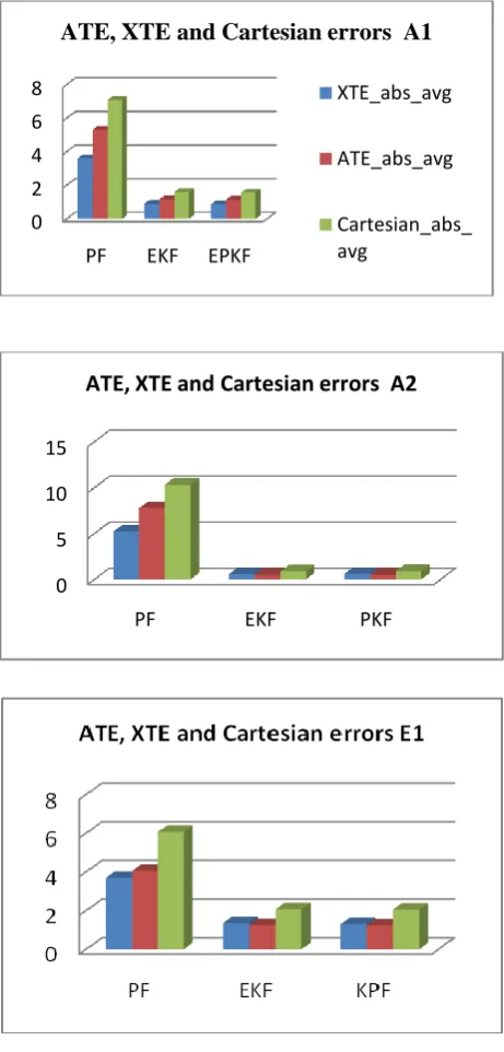
The results are summarized graphically using bar chart in Fig [4]. Chiefly, we consider the cross-track error (abbreviated XTE), which gives the component of position error that is orthogonal to the robot’s path. We also present the along-track error (abbreviated ATE), which measures the tangential component of position error.

0 2 4 6 8

PF EKF EPKF

ATE, XTE and Cartesian errors A1

XTE_abs_avg

ATE_abs_avg

Cartesian_abs_ avg

0 5 10 15

PF EKF PKF

(7)

Fig.5: The EKF, the Enhanced EPKF and PF along-track error, the cross-track error and Cartesian errors

From Table [1-7] and fig [5] comparable results we notice the slight difference in calculated error among extended kalman filter and the proposed enhanced particle / kalman filter while the particle filter posses excessive error.

Considering computational complexity and time consumed in a Matlab run, Fig [6] shows the time consumed by each filter in the same environmental Conditions. There is a slight increase in time for the propose EPKF compared with EKF while the PF consumes higher time. Therefore, the proposed filter achieves the same results of EKF while keeping the computational cost reasonable and in the same time solving the problem inherent of all Kalman filters which require a defined initial state.

Table.8 Summarizes the Average Time each Algorithm Requires to Incorporate an Incoming Range Measurement

into the Robot Position Estimate

Running Times seconds per

measurement update

Particle Filter 0.142494

EKF 0.007988

EPKF: PF estimate an initial state which to seed the EKF.

0.014385

Fig.6: Comparing the time required to update the robot pose estimate after a range measurement is taken.

5. CONCLUSION

This paper presents a study for the effect of several filter approaches in the behavior of robot localizer using radio beacons that provide the ability to measure range only. Different filters namely Extended Kalman Filter (EKF), Particle Filter (PF) and a proposed Enhanced Particle/Kalman Filter (EPKF) are implemented in Matlab environment and their behavior are evaluated. The Enhanced Particle/ Kalman Filter (EPKF) provide the required initial location while there is no significant change in the computational cost compared with Extended Kalman Filter (EKF). Moreover in some data sets, the performance of the proposed filter approach is superior in terms of localization errors.

6. ACKNOWLEDGMENTS

I would like to express my deep sincere thanks to Prof. Dr. Imbaby Ismail, Prof. of Electronics and Communications Engineering for effective supervision, great help, encouragement as well as fruitful discussions throughout the progress of this work.

I would like to thank Dr. May salama, for her great support, patience, and encouragement.

0 1 2 3 4

PF KF PKF

XTE,ATE and Cartesian errors E3

XTE_abs_avg

ATE_abs_avg

Cartesian_abs _avg

0 1 2 3 4

PF EKF PKF

(8)

7. REFERENCES

[1] Fox, D. (1999). Markov localization for mobile robots in dynamic environments, Journal of Artificial Intelligence Research: 391-427.

[2] Maskell,S., Gordon,N. and Clapp T February 2002, A Tutorial on Particle Filters for Online Nonlinear/Non-Gaussian Bayesian Tracking, IEEE Transactions on Signal Processing, 50( 2):174-188,

[3] Ioannis ,R. 2004. A particle filter tutorial for mobile robot localization, Technical Report TR-CIM-04-02,McGill University, Canada.

[4] http://oursland.net/projects/fastslam/

[5] Carpenter,J. and Clifford,P. and Fearnhead,P. 1999 An Improved Particle Filter for Non-linear Problems Department of Statistics, University of Oxford.

[6] Maskell, S., Gordon,N. and Clapp,T. 2002, A Tutorial on Particle Filters for Online Nonlinear/Non-Gaussian Bayesian Tracking, M. Sanjeev Arulampalam, IEEE Transactions on Signal Processing, Vol. 50, NO. 2. [7] Thrun,S., Fox,D., Burgard, W. and Dellaert, F. 2000

Robust Monte Carlo localization for mobile robots, Artificial Intelligence, pp. 99-141.

[8] Liu, J. and Chen, R.1998 Sequential Monte Carlo methods for dynamic systems, Journal of American Statistical Association, 93.

[9] Doucet,A., de Freitas,N., and Gordon,N.,2001. Sequential Monte Carlo Methods in Practice, Springer. [10]Sasiadek, J. Z. and Hartana, P. 2000 Sensor data fusion

using Kalman filter, InProceedings of the Third International Conference on Information Fusion, vol. 2,pp. 19-25.

[11]Djugash,J. and Singh.S 2009 A Robust Method of Localization and Mapping Using Only Range The Robotics Institute, Carnegie Mellon University, Pittsburgh, PA 15213, USA

[12]Y. Bar-Shalom, X. Rong Li, and T. Kirubarajan, Estimation with Applications to Tracking and Navigation, 2001.

[13]Abd El-Halym, H. A, Mahmoud, I. I., AbdelTawab.A, and Habib, S.E.D. 2009 Appraisal of an Enhanced Particle Filter for Object Tracking, Proceedings of IEEE International conference on Image processing (ICIP) Conf., Cairo, Egypt, pp. 4105-4107.

[14]Ristics, B., Arulanpulam, S. and Gordon, N. Beyond the Kalman Filter, Artech House, 2004.

[15]Abd El-Halym, H. A. E.-L., Mahmoud, I. I., and Habib, S. E. D. 2012. Proposed hardware architectures of particle filter for object tracking. EURASIP Journal on Advances in Signal Processing, 1(17), 1-19.

[16]Abd El-Halym, H. A, Mahmoud, I. I., AbdelTawab.A, and Habib, S.E.D. 2009 Particle Filter versus Particle Swarm Optimization for Object Tracking,proceedings of ASAT Conf,Cairo Egypt

[17]Isard. M. and Blake,A. 1998 Condensation –, conditional density propagation for visual tracking, International Journal of Computer Vision 29(1), pp. 5-28.

[18]Kurth,D.2004 Range-Only Robot Localization and SLAM with Radio, Robotics Institute, Carnegie Mellon Univ., Technical Report CMU-RI-TR-04-29