Static Traffic Assignment with Queuing

(1)

Static Traffic Assignment

with Queuing

Master Thesis Applied Mathematics

(2)

Static Traffic Assignment with Queuing

A.S. van Leeuwen

0067857

University of Twente

Applied Mathematics

Industrial Engineering and Operations Research

Discrete Mathematics and Mathematical Programming

Graduation committee:

Dr. G.J. Still (University of Twente)

Dr. W. Kern (University of Twente)

Prof. Dr. M.J. Uetz (University of Twente)

(3)

iii

Abstract

Traffic models are used to predict traffic flows and travel times on a road network. Due to the ever increasing level of congestion at highways and urban areas, the need for better results from those models also increases. On the other hand, these predictions should be available in a reasonable time such that the right action to avoid congestion can be taken quickly. Because of computation time issues, often static models instead of dynamic models are used.

For realistic predictions a traffic model should be able to take capacity constraints into account, something that traditional static traffic assignment models cannot do directly. Besides that, queuing and spillback phenomena should also be taken care of. In this thesis, an overview is given of the static models and concepts in literature that in some way or another do account for capacity limitations and/or spillback effects. It is explained that all of these models still have drawbacks, and therefore a new static traffic assignment model is introduced.

This new model is basically obtained in two successive steps. First the static variant of the dynamic network loading model LTM (Link Transmission Model) by Yperman (2007) is derived by assuming stationary traffic demand. After that, the STAQ (Static Traffic Assignment with Queuing) model is created by assuming instantaneous traffic flow propagation.

(4)

iv

Preface

This thesis is the result of my research at Goudappel Coffeng B.V. and the University of Twente on static traffic assignment models. I worked for about 10 months on this research, which was done at the chair of Discrete Mathematics and Mathematical Programming.

I would like to thank my supervisors at Goudappel in Deventer, Luuk and Michiel, for the daily guidance during the research. They were always willing to discuss problems and gave many suggestions for improvements.

Also I would like to thank Walter and Georg, my supervisors at the university. Though sometimes I had difficulties explaining the idea and the workings of the model, they were very helpful with improving my report.

(5)

v

Introduction

Traffic models are widely used as a tool to assist in making decisions in mobility and infrastructure planning. These tools can help in analyzing congestion issues, and can predict the consequences of certain measurements, like adding an extra lane, building a new road, raising the maximum allowed speed or applying road pricing.

A classical traffic model to predict traffic flows is known as the four step model. The four steps are trip generation, trip distribution, modal split and assignment. In this model the network is divided in zones, between which people can travel. The first step is the trip generation. Based on data about the population and economic activity like employment, shopping space, educational and recreational facilities at a zone, the total number of trips generated at each zone and the number of trips attracted by each zone is estimated. At the next step, these trips are distributed over space, resulting in a OD-matrix (origin-destination matrix). An OD-matrix contains the number of trips from each origin to each destination (zone). The third step is called modal split, in which the trips are allocated to different modes of transport, for instance car, public transport, or bike. In the last step, the assignment of the trips to the network links is done. Basically this means that for each OD-pair, the number of trips is distributed over a number of routes (or paths) which consists of a number of links in sequence. This gives the number of vehicles that want to travel over each link, i.e. the demand for each link.

Traffic models can be either static or dynamic. Within dynamic models, the traffic demand (OD-matrix) can change through time, while within a static model it is assumed that the traffic demand is constant through time.

In this thesis, the focus will be on the assignment phase of the process of a static traffic model. As the mode of transport, only car is considered. It is assumed that an OD-matrix is available.

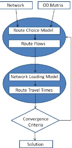
[image:7.595.323.473.428.734.2]

The assignment phase of the traffic model consists of two components (see Figure 1). The first component is the route choice model, in which routes are selected and the traffic demand is assigned to these routes. The second component is the network loading model, which takes the assigned route flow as input and describes the way in which the traffic is propagated through the network. The network loading model yields the link flows which can be used to determine the route travel times.

(8)

2

1.1.

Motivation of research

With the ever increasing level of congestion it becomes more and more important that the traffic model predictions are as accurate as possible, but on the other hand the computation time should be as low as possible such that these predictions can be achieved very fast. Dynamic models can produce realistic predictions with consistent congestion formation and delays, but in general take much more time to compute than static models. On the other hand, current static models can compute a result very fast, but these models usually cannot handle congestion effects correctly as these effects are time dependent in nature. Therefore, there is need for a quasi-dynamic model, that produces realistic travel times but is still computational attractive.

1.2.

Research questions

In this thesis it will be investigated whether a traffic assignment model can be formulated that can produce realistic travel times in a static or quasi-dynamic context and can generate these results in a reasonable time. To accomplish this objective, the following research questions are formulated. At first in the existing literature will be searched for a model that complies with the demands mentioned before:

1. Are there static traffic assignment models in the literature that can deal with congestion and can compute realistic travel times?

If such a model cannot be found, the goal is to specify such a model:

(9)

3

1.3.

Overview of the thesis

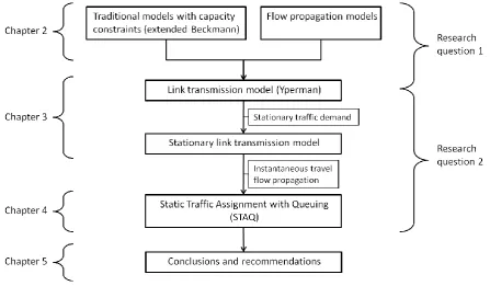
In Figure 2 a schematic overview of the thesis is given. In the next chapter, the first research question is answered. A summary is given of the different static traffic assignment models that can deal with capacity constraints. The different approaches are discussed and the choice to derive a new model from the dynamic Link Transmission Model (LTM) by Yperman (2007) is motivated.

In chapter 3, the working of the LTM by Yperman is presented. It is explained how the LTM is used as the basis of the new model. After that the quasi-dynamic variant of the LTM with stationary traffic demand is derived.

The subject of the fourth chapter is STAQ: Static Traffic Assignment with Queuing, the newly developed model at Goudappel Coffeng B.V. The model uses elements from the LTM by Yperman, with some additional assumptions. The most important additional assumption is that of instantaneous travel flow propagation. The derivation of STAQ from the LTM with stationary demand is showed and an algorithm is presented which can solve the STAQ model efficiently.

[image:9.595.73.521.318.579.2]

Finally some conclusions and recommendations for further work are given in the last chapter.

(10)

(11)

5

(1)

2.

Traffic assignment models with capacity constraints: A summary

In this chapter an overview is given of different traffic models that somehow can deal with capacity constraints. All the models considered here provide a method to predict the traffic flow on the links, given a network and an OD-matrix with traffic demand. From this information the travel times can be determined.

The traffic demand needs to be assigned to the links in the network in a certain way. To obtain realistic results, the capacities of the links in the network and the congestion that it can cause must be taken into account. In this overview different approaches are discussed that are proposed in the literature. In the first part, the traditional approach is explained, that does not take the capacity constraints into account. After that, the traditional approach extended with capacity constraints is discussed, with a number of different solution techniques. Then some other, more realistic ideas are presented. Finally the advantages and disadvantages of the models are discussed and it is explained what qualities the new model should have.

2.1.

Traditional static traffic assignment

Wardrop’s first principle (Wardrop 1952) states that at an equilibrium situation the travel times of all routes between each OD-pair actually used are the same, and there are no unused routes with a lower travel time. This means that no user can lower his travel time by switching individually to another route. To find an equilibrium solution in a network, the problem can be described in a mathematical way (Beckmann e.a. 1956).

Consider a network given by a set of nodes (or vertices) and a set of links (or edges) . The set consists of the origin-destination (OD) pairs , with a demand , for each OD-pair. Furthermore, is the set of directed routes (or paths) for OD-pair with

. The objective is to find a traffic flow through the network, that satisfies the demand

for each OD-pair, by assigning a certain amount of nonnegative flow to each link . More formally, find an satisfying:

where consists of the path flows for each path , and the incidence matrices

_and _{are defined as follows:}

(12)

6

(2) The set of feasible flows consists of all traffic flows (with a corresponding ) such that (1) is satisfied for demand .

For each link is usually defined a link cost function or travel time function (separable) or more general (non-separable cost function). In the separable case, the link cost is only dependent of the flow on the link itself. Usually it is assumed that the link cost functions are continuous and monotonically non-decreasing in the link flows. So, more flow means higher link costs. The function named after the United States Bureau of Public Roads (BPR function) is frequently used as a cost function:

where is the free flow travel time on link , is the capacity of link in vehicles per time unit and and are adjustable parameters (US Bureau of Public Roads 1964).

A common assumption is that the path costs are additive:

A given feasible traffic flow is called a Wardrop Equilibrium flow if the following holds:

Or, equivalently:

So, when a given feasible flow assigns a positive flow on a certain path, the costs on that path cannot be greater than the costs on any other path for the corresponding OD-pair. In other words, if a cheaper alternative exists for a certain path, that path will have zero flow assigned:

If the cost functions are separable, the equilibrium solution can be found by solving the following Beckmann User Equilibrium optimization problem (Beckmann e.a. 1956). This formulation is in general not possible if the cost functions are not separable.

subject to (1)

Because the set is compact (closed and bounded), the (continuous) objective function will reach its minimum, so the existence of a solution is guaranteed. If all cost functions are continuous and non-decreasing, this optimization problem is convex and then it can be showed that a solution

(13)

7

not (strictly) convex in the path flows, so there may be more than one path flow pattern that generates the unique link flow solution. (Yang & Huang 2005)

The necessary and sufficient first order optimality conditions (Karush Kuhn Tucker conditions) for an optimal path flow vector are as follows (Yang & Huang 2005):

Here is the vector of Lagrange multipliers for the demand constraints corresponding to the OD pairs. It follows that for all

and

This corresponds to the definition of a Wardrop Equilibrium. can be interpreted as the equilibrium (minimal) path cost for OD pair .

When the cost functions are non-separable, in general the problem cannot be written in the Beckmann formulation. However, it can be formulated as a Variational Inequality Problem (VIP):

where is the vector of link costs for each link for link flows .

If the link cost functions only depend on the flow on the link itself (separable cost functions), the VIP is equivalent to the Beckmann minimization problem.

The standard Beckmann model can be solved for instance with a Frank-Wolfe type algorithm. This method converts the problem into a series of shortest path subproblems which can be solved relatively easy. Most solution methods exploit the Cartesian product structure of the feasible solution set. The idea is as follows:

(14)

8

(3) 2. (Iteration) Find a feasible search direction by finding the shortest paths.

3. Find the optimal step size (line search) in this direction.

4. Update the link flows.

5. If the convergence criterion is not met, continue at step 2.

2.2.

Traditional static traffic assignment with capacity constraints

The classical Beckmann model as described in the previous section does not take link capacities explicitly into account and therefore can produce unrealistic flows. Assigning more flow to a link than its capacity is penalized by the monotonically non-decreasing travel time function, but it is not forbidden. Numerous ideas and suggestions have been given in the literature to deal with link capacities. One can use travel time functions with vertical asymptotes at the capacity. However, this method is not favorable because it can produce unrealistically high travel times when flow approaches capacity and can give numerical problems (Larsson & Patriksson 1995). Therefore in this overview the focus is on models that have explicit link capacity constraints.

By adding simple capacity constraints to the Beckmann optimization problem, the capacitated (or extended) Beckmann User Equilibrium optimization problem is obtained. (Larsson & Patriksson 1995, Nie e.a. 2004)

subject to (1) and

The necessary and sufficient first order optimality conditions (Karush Kuhn Tucker conditions) for an optimal path flow vector are as follows (Yang & Huang 2005):

(15)

9

Here

are called the generalized path costs, and

are the generalized link costs. The vector is the vector of Lagrange multipliers for the demand constraints corresponding with the OD pairs, which can be interpreted as the vector of equilibrium generalized path travel times. Similar to the standard Beckmann model, it holds for all

that

if

and

if

Furthermore, is the vector of Lagrange multipliers for the capacity constraints of each link. can be seen as the equilibrium queuing delay time, an additional time penalty that users traveling on this link are willing to wait for continuously using this link (Yang & Huang 2005). This delay time can only be positive when the link flow equals the link capacity. While there is a unique solution for the vector of equilibrium generalized path travel times , the vector of delay times is in general not unique. Therefore, not too much importance should be given to these delay times (Nie e.a. 2004). The capacitated Beckmann optimization problem is not capable to handle spillback, since there are no physical queues created. Spillback (or blocking back) is the phenomenon that a queue will continue on the preceding links when it reaches the link end. Within the capacitated Beckmann problem, only a time penalty is given to the links that are ‘congested’, i.e. to the links that have an assigned traffic flow that is equal to the capacity.

(16)

10

2.2.1. Interior penalty function approach

The interior penalty function (IPF) approach tries to approximate the capacity constrained traffic assignment problem by adding a penalty term to the objective function of the “unconstrained” problem. By imposing an asymptotic penalty term when the link flow approaches the link capacity, it is prevented that an infeasible solution is achieved. An initial feasible solution is necessary for this approach. Within optimization theory, this approach is known as the barrier method (see e.g. Faigle e.a. 2002). The optimization problem becomes:

Here is the penalty parameter, is a penalty function that is continuous on for all

and

when

In principle, the problem can now be solved as a standard Beckmann program. The sequence of solutions will converge to the optimal solution of (3) as .

Examples of penalty functions in the IPF approach:

Nie e.a. (2004)

Prashker & Toledo (2004)

Note that the penalty functions of Nie e.a. and Prashker & Toledo are in fact identical:

(17)

11

2.2.2. Augmented Lagrangean dual with exterior penalty function approach

In this approach, also an extra term is added to the objective function. By imposing a penalty term when the flow of a link is greater than the link capacity, the method forces the sequence of solutions into the feasible area. An initial feasible solution is not necessary. The optimization problem becomes, similar to the interior penalty function approach:

(

4

)

where is a penalty function, with for all and if and only if

, and is continuous on . Now the penalty subproblem is an uncapacitated traffic assignment problem again. Let the solution of (4) for penalty parameter be . It can be showed that (under certain assumptions) for all , and , where is

the optimal solution of the capacitated Beckmann problem (3) (Larsson & Patriksson 1995). So, the sequence of solutions will converge to the optimal solution of (3) as . An example of a penalty function is:

Because of the condition the problem becomes ill-conditioned. This is inherent in the penalty approach. To avoid this, a Lagrangean term is added to the objective function, creating an augmented Lagrangean function (for the penalty function above): (Larsson & Patriksson 1995)

(

5

)

Let be the solution of the subproblem (5) with penalty parameter and vector of Lagrangean dual variables for the capacity constraints. It can be showed that for large enough: there exists an optimal Lagrange multiplier such that

, and .

Compare (part of) the KKT conditions of the capacitated Beckmann problem (3)

and the augmented Lagrangean (5):

with is a vector with elements for each . It

follows that the sequence of Lagrange multipliers should be updated as follows:

(18)

12

It follows that if then the condition is no longer needed for convergence, so the problem is no longer ill conditioned.

2.2.3. Dynamic penalty function approach

In the method of Shahpar e.a. (2008), the capacity constraints are taken into consideration by implicitly adding a penalty function to the link travel time functions, which they call a dynamic penalty function. They let a penalty term

play the role of the Lagrangean multipliers for the capacity constraints in the KKT conditions (based on Larsson & Patriksson (1999)). Here is the th side constraint and is a interior penalty function. For general side constraints the generalized path costs now become:

The simple capacity constraints are reformulated as for all .

For details see Shahpar e.a. (2008). They tested their algorithm on some small and medium sized networks for the simple capacity side constraints. Their experiments achieved a solution for the link capacity constrained problem faster than the interior penalty function method or the augmented Lagrangean method.

2.2.4. Conclusion

All the above described solution techniques can solve the capacitated Beckmann optimization problem. Though the capacitated Beckmann problem has a nice mathematical formulation, in general it cannot give realistic results, since queuing and spillback effects are not taken into account. It is known from practice that congestion on a link can have consequences for traffic flow on upstream links. Besides that, the travel time functions used by these models are difficult to determine and need time for calibration. Therefore, in the next section other approaches that avoid the use of these functions are discussed.

2.3.

More realistic static traffic assignment

(19)

13

2.3.1. Stable equilibrium model

Nesterov & De Palma (e.g. 2000, 2003) introduce a theory of static equilibria in congested networks, the stable equilibrium model. They observe that if the flow on a link is small, then either little traffic is using it (low travel time), or the link is heavily congested (high travel time). They state that the assumption that the travel time is an increasing function of the flow as is done within the extended Beckmann formulation is artificial. Nesterov & De Palma use the fundamental relation between the flow rate (intensity), travel time and the loading (density) on a link: flow = speed x density (see also section 3.2 about the fundamental diagram).

They obtain stable equilibrium solutions only by imposing lower bounds on the travel time (the free flow travel time) and upper bounds on the flow (the link capacity). They assume that if the flow on a link is strictly smaller than the capacity, then there is no congestion and the equilibrium travel time on this link is equal to the minimal (free flow) travel time. If the link flow is equal to the capacity, then the equilibrium travel time is greater or equal then the minimal travel time. In this case there is congestion on the link. In fact this could be defined as a travel time function as follows:

Here is the free flow travel time on link and .

A Nesterov Equilibrium solution satisfies the following conditions: and , and is a Wardrop Equilibrium with respect to . Kern & Still (2009) show that the idea of Nesterov & De Palma can be seen as a special case of a generalized Wardrop Equilibrium, and that it can be extended to the non-separable case.

The model of Nesterov & de Palma is not capable of handling spillback. They propose to add an extra condition such that the length of the queue on a link cannot exceed the link length by stating that

, where is the link length and the average length occupied by a vehicle. However, in the rest of their papers they do not use this condition; they just assume that spillback never occurs, so it is unclear what the effect is of this condition in the model.

Chudak e.a. (2007) compare the Nesterov & De Palma model with the (extended) Beckmann model on some small networks. However, it is not clear which of the models better predicts the real traffic flow. Real data from traffic counters is needed to be able to draw hard conclusions..

2.3.2. Flow propagation models

In this section some flow propagation models are described. Four models are considered: the model by Bifulco and Crisalli (1998), the model by Bundschuh e.a. (2006), QBLOK by 4Cast (2009) and the Link Transmission Model by Yperman (2007).

(20)

14

They assume that for a certain OD-pair, each path has a certain probability to be taken by a user, depending on the path cost vector of that OD-pair. In their model, they determine iteratively which quantity of users on a link can proceed to the next link on their path, by checking the link capacities. This results in a new link flow pattern that is used in the next iteration. The algorithm stops when a stable link flow solution is established, which is close enough to the previous iteration. More precisely they state:

Where the -element of indicates the percentage of the flow on path that is allowed to reach link , taking capacity constraints into account. The -element of indicates the probability of choosing path for OD pair . is the demand vector. By iteratively updating the link flow vector and the matrix, the flow vector will converge to the final solution.

Bundschuh e.a. (2006) propose a flow propagation method to determine congestion in a static assignment model. They call their model quasi-dynamic, since it does account for capacity limitations and spillback phenomena, but requires less computation time than a dynamic model. They assume a time period for which the static situation is valid. The method consists of two phases. In the first phase the traffic is propagated through the network, taking into account the link capacities. In the second phase the delay times are calculated.

The flow propagation is done in fractions. Dividing the flow in fractions reduces the influence of the order in which the routes and OD pairs are handled. The flow is propagated over the consecutive links of a route until the capacity of a certain link is reached. The extra flow on that link that cannot continue will be stored in the queue. Each link has a queue capacity, the maximal queue length in number of vehicles. If this amount is reached, and still more flow is propagated over this link, the surplus (i.e. spillback) is moved back to the preceding link(s) along the route.

In the second phase, the delay times are computed by determining the time it takes to empty the queues on the links in the network after the first phase while no extra flow is added. This is also done in steps by dividing the bottleneck link capacity into fractions.

In their model, Bundschuh e.a. introduce a permeability factor. This rule allows traffic to pass a queue that has spilt back, if the traffic follows a route that does not go through the link that caused the queue. This can happen for instance in the presence of separate turning lanes. The factor determines the fraction of traffic volume that is able to pass the queue.

It is not clear how Bundschuh e.a. determine the queue capacity. They assume that a vehicle always requires the same space within a congested link. However, it is known from the fundamental diagram (see section 3.2) that this is not true: the density (in vehicles/km) of a congested link is dependent of the flow (vehicles/hour). If the link is congested and there is only a little flow then the density is very high, but if there is only a little congestion and the flow is close to the link capacity, then the density is much lower. Surely Bundschuh e.a. take either the value of the critical density (density at capacity flow) or the jam density (fully congested, zero flow), or some value in between, but in general the queue length will not be accurate.

(21)

15

QBLOK (4Cast, 2009) is a traffic assignment algorithm that is used in practice in the Netherlands. Based on the capacity, travel demand and route choice behavior, the model assigns the traffic to the network. Route choice behavior is based on the first Wardrop principle. The model does account for congestion and spillback phenomena. The model does have some drawbacks. It can produce unrealistic travel times and strange route choices. The model uses a heuristic approach to reach an equilibrium situation by setting a predefined number of iterations and mixing the resulting link flows from different iterations according a certain distribution. It is not a mathematical model, but merely an algorithm that tries to find a satisfying result.

The Link Transmission Model (LTM) by Yperman (2007) is a dynamic network loading model designed for the dynamic traffic assignment problem. It describes the traffic propagation through a network in a realistic way (consistent with kinematic wave theory) and determines the link flows, densities and travel times. It does account for link capacities and spillback phenomena. The route flows from an existing route choice model are the input for the link transmission model. The model is built for the dynamic traffic assignment problem, but it is useful as a starting point for a static model.

2.4.

Discussion

The attention for capacitated static traffic assignment that do account for queuing and spillback effects is scarce in the literature. In the table below, the different mathematical models that have been discussed in this chapter are categorized.

Mathematical Model Solution Method Implementation

Extended Beckmann User Equilibrium (with link capacity constraints)

Augmented Lagrangean dual with exterior penalty function

Larsson & Patriksson 1995

Nie e.a. 2004

Interior penalty function Nie e.a. 2004

Prashker & Toledo 2004

Dynamic penalty function Shahpar e.a. 2008

Stable Dynamics n/a Nesterov & De Palma

2000&2003

Flow propagation model Propagate demand iteratively through the network

Bifulco & Crisalli 1998

Bundschuh e.a. 2006

Yperman 2007 (dynamic)

[image:21.595.71.527.418.694.2]

4Cast 2009

Table 1. Overview of different mathematical models that can deal with capacity constraints

(22)

16

follow the traditional approach and combine the route choice model and the determination of the link flows in the extended Beckmann optimization problem. The advantage of the (extended) Beckmann formulation is that it has a nice mathematical form, which can be solved using different solution techniques. However, those methods do not model the formation of queues and spillback (or blocking back) effects are not taken into account. It merely adds a time penalty for using a link that is filled to the capacity. However, since it is known from practice that congestion on a link can have consequences for the traffic flow on preceding links, these effects must be accounted for. Another disadvantage of the extended Beckmann formulation is that when a link does not have enough capacity, the travel time of that link will increase, instead of the travel time of the link(s) before that link. Besides that, most of these models apply travel time functions, which are in practice hard to determine and in general require time to calibrate to resemble acquired traffic counts.

There are some papers that try to obtain more realistic results. The Stable Dynamics model by Nesterov & De Palma uses only upper and lower bounds on the link flow and travel time respectively and utilizes the fundamental diagram to find a stable equilibrium. They propose adding an extra condition to deal with spillback. Unfortunately, in the rest of their work they do not use this condition; they just assume that spillback never occurs, so the effect of this condition in the model is unclear.

Bifulco & Crisalli (1998), Bundschuh e.a. (2006) and Yperman (2007) describe a flow propagation model (which contains no route choice model), taking a path flow vector coming from an existing route choice model as input. Bifulco & Crisalli describe a method to iteratively propagate the flow through the network by computing the fraction that is able to continue on the path given the link capacities. However, their model cannot handle spillback.

Bundschuh’s model is a practical model that does account for spillback, but there are some drawbacks: they start building the queue in the bottleneck link instead of before the link. Besides that, they imply that the queue capacity of a link is constant. However, the queue capacity depends on the density of the queue.

QBlok does account for queuing and blocking back phenomena. However, this method is merely an algorithm using heuristics and if-then structures, and can result in strange route choices and unrealistic travel times. Since it is not a mathematical model, nothing can be said beforehand about the results either.

The dynamic Link Transmission Model (LTM) by Yperman (2007) does account for spillback effects, and describes the propagation of traffic flow through the network according to kinematic wave theory. Since the model is based on kinematic wave theory, it has a mathematical basis. Kinematic wave theory is considered as good method to model first order traffic flows.

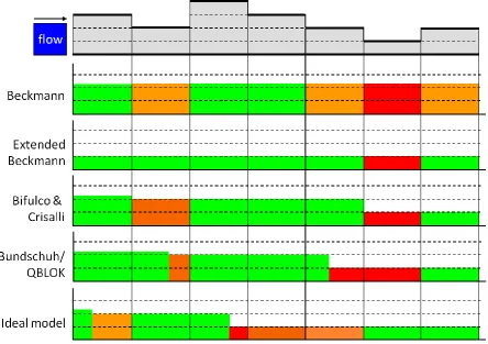
In the figure on page 17, differences between some of the models are shown in a small hypothetical network. It gives an idea of the differences of the standard Beckmann model, the extended Beckmann model, the model Bifulco & Crisalli, the model of Bundschuh e.a. and QBlok. Furthermore it is shown how an ideal model should work.

(23)

17

[image:23.595.81.526.164.477.2]

If this is the only route on this network, the extended Beckmann model shall not have a feasible solution, because in some links there is not enough capacity. Therefore, it is assumed that there is an alternative route with unlimited capacity starting from the origin (upstream end of the first link) and ending at the destination (downstream end of the last link), with a very high travel time. In this way, this alternative route will only be chosen when there is no other option.

Figure 3. Comparison of traffic flows and speeds between different static models.

In the standard Beckmann model, where capacities are not taken into account, all link flows are equal to the input flow and are overestimated, and the travel times will be higher in the saturated links. In the extended Beckmann model, because of the low capacity of the sixth link, the flow on the whole route will be low and underestimated. The rest of the flow will be assigned to the alternative route. The travel time of the bottleneck link will be higher than in the other links. The third part of the figure shows the idea of the model Bifulco & Crisalli. The traffic flow pattern here is more realistic, but the queues are built inside the bottleneck links and spillback cannot occur. The fourth part shows the model by Bundschuh e.a. and the model QBLOK. Queues will appear inside the bottlenecks, and possibly spillback occurs. Both models work differently, but yield comparable results. It should be mentioned that unlike Bundschuh’s model, QBLOK is merely a heuristic and not a complete model.

(24)

18

2.5.

Conclusion

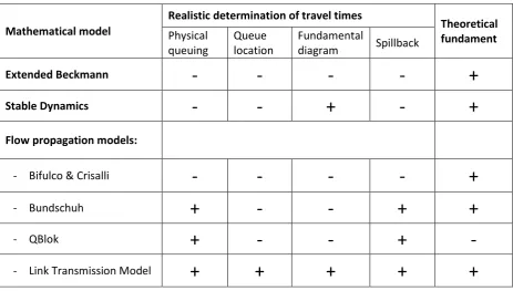
In this chapter different models and approaches from the literature were discussed and compared. The models are compared on the realism of the determination of the travel times and the mathematical or theoretical fundament the models are based on. The realism of the travel times is divided into four criteria (see Table 2).

Mathematical model

Realistic determination of travel times

Theoretical fundament

Physical queuing

Queue location

Fundamental

diagram Spillback

Extended Beckmann

-

+

Stable Dynamics

-

+

-

+

Flow propagation models:

- Bifulco & Crisalli

-

+

- Bundschuh

+

-

+

- QBlok

+

-

+

-

[image:24.595.66.530.178.441.2]

- Link Transmission Model

+

Table 2. Summary of the comparison of the different approaches in literature on a number of criteria.

(25)

19

3.

Link Transmission Model

The Link Transmission Model by Yperman (2007) is a dynamic network loading model that is used for the dynamic traffic assignment. The model realistically describes traffic propagation on a network. In this chapter the working of the Link Transmission Model (LTM) is described. In the first section the basic idea is explained. In the sections thereafter, the theory about the fundamental diagram, kinematic wave theory and shock wave theory is described shortly, to support further explanation of the model.

In the seventh section, an event-based, dynamic variant of the LTM is derived. It is called quasi-dynamic because it is assumed that the route flows are stationary, i.e. constant over time. Through this assumption, the model becomes less complex and far less calculations are needed. This adjusted, stationary Link Transmission Model is used as a step towards the Static Traffic Assignment with Queuing (STAQ) model, which will be the subject of chapter 4. In the last section an algorithm for the stationary LTM is presented.

3.1.

Introduction to the LTM by Yperman

The original LTM is a dynamic network loading model. It is a simulation model that describes how the traffic propagates through the network over time in a realistic manner, consistent with the fundamental diagram and kinematic wave theory (see the next sections). It takes as input the time dependent route flows obtained by some existing route choice model. The LTM is the second component of a Dynamic Traffic Assignment model as illustrated in Figure 1 on page 1.

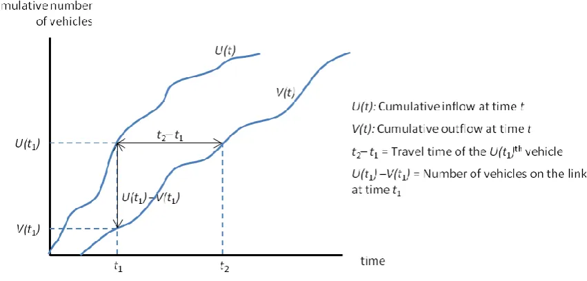
The LTM determines link volumes (i.e. number of vehicles) and travel times given the route flows. A route flow is loaded onto the network in the origin node and after some time leaves the network through its destination node.

The LTM counts the cumulative number of vehicles that have passed the beginning and the end of each link at time . The number of vehicles that have passed location at time is . Location is the start of a link and location is the end of the link, where is the link length. So, the cumulative number of vehicles that have entered a link (cumulative inflow) at time is . Similarly, represents the cumulative number of vehicles that have left a link (cumulative outflow) at time . By cumulative number of vehicles is meant the total number of vehicles since the start at time . To simplify notation, is used for the cumulative inflow and

for the cumulative outflow. It is assumed that there is no overtaking on a link (First In First Out behavior).

The cumulative in- and outflow can be visualized as in Figure 4. The difference between the time a vehicle entered and the time it left a link is the link travel time of that vehicle. The difference between in- and outflow is the number of vehicles on a link at a certain moment in time. So, if

(26)

[image:26.595.90.516.77.281.2]

20

Figure 4. Example of cumulative in- and outflow curves of a link over time.

The LTM is a time based algorithm. For each time step (of fixed size), it determines for each link which amount of vehicles in that time step moves on to the next link, and adds this amount to the respective cumulative in- and outflows. To do this, the LTM uses the concept of sending, receiving and transition flows. The LTM can be divided into two parts: the link model and the node model. In the node model it is determined which part of the traffic that wants to go towards a certain link is actually allowed to go to that link, based on the available capacities of the links connected to that node. In the link model, the traffic is propagated over a link in such a way that it is consistent with kinematic wave theory. A brief introduction to kinematic wave theory is given in section 3.3. Within kinematic wave theory, it is assumed that the fundamental relation between traffic flow (intensity), speed and density holds. This relation is described in a fundamental diagram. The fundamental diagram is the subject of the next section.

3.2.

Fundamental diagram

A fundamental diagram describes the relation between the three important entities within traffic flow theory:

traffic flow rate, intensity of the traffic (vehicles/hour)

the density (German: konzentration) of the traffic (vehicles/km) the speed (velocity) of the traffic (km/hour)

The relation is known as the fundamental equation of traffic flow. This equation is based on the assumption that on average, drivers will drive the same under the same average conditions: at a certain speed , they remain the same distance headway with respect to the next vehicle on the road. Each link can have a different fundamental diagram, but the diagram remains the same over time.

(27)

21 Speed – density:

Speed – intensity: Intensity – density:

The diagram showing the intensity – density relation is the most convenient for this thesis. In literature, different forms for the fundamental diagram have been proposed. One of the simplest forms is the diagram proposed by Newell (1993) and by Daganzo (1994) (Figure 5a). The intensity – density graph consists of two straight lines. From this graph, the speed at a certain density can be found, by determining the slope of the line from the origin to the point on the graph at that density (i.e. ). The part of the diagram that lies to the left of the critical density (increasing part of the diagram) is the uncongested part, in this part the traffic can flow with the free flow speed . At the critical density, the flow rate is equal to the capacity of the link, indicated by . When the road traffic becomes more dense than , both the flow that can go through the link and the speed of the flow decreases, until it reaches the jam density . At that point, no flow is possible, so the speed is zero. Note that the diagram is determined by only three parameters: the free flow speed , the capacity , and the jam density . The slope for the congested wave speed follows from these parameters by .

a

[image:27.595.111.479.364.725.2]

b

(28)

22

Smulders (1990) introduced an similar form of this diagram, but he introduced a parabolic curve at the uncongested part (Figure 5b). This is a slightly more realistic way to model the speed in an uncongested link, because when the road becomes denser, speed will decrease: at the capacity flow, the speed is strictly less than the free flow speed ( ).

Like in Yperman (2007), Newells diagram (Figure 5a) is used in this thesis, because the diagram has some nice mathematical properties. Only two possible kinematic wave speeds exist (see section 3.5): the free flow speed for uncongested conditions (slope of first straigth line) and for congested conditions (slope of second straight line).

3.3.

Kinematic wave theory

The function for the cumulative vehicle numbers at location and time is in general discontinuous, since the number of vehicles is discrete. Therefore it is assumed that a smooth approximation of the cumulative number of vehicles is available such that the function is twice differentiable. The approximation should coincide with the original function at the positions where a vehicle enters or exits the link, i.e. the ‘steps’ in the function. In this way the partial derivatives of

can be determined. The partial derivative with respect to can be interpreted as the instantaneous flow (in vehicles per time unit) at point :

The partial derivative with respect to can be interpreted as the density (in vehicles per kilometer) at point :

The density has a negative sign because for increasing , is decreasing. It is assumed that our smooth approximation of has continuous second partial derivatives, so the identity

yields

(

6

)

This equation is known as the conservation law. It ensures that changes in the rates of the flow and density over time and space cannot cause vehicles to appear or disappear.

(29)

23

(

7

)

Now the conservation law is formulated with only one independent variable, the density . In the following, is used to represent the value of the derivative of , . Since a fundamental diagram with two linear segments is used (Figure 5a), only two different values for can occur: the free flow wave speed and the congested wave speed . As long as is constant, solutions of the partial differential equation

(

7

)

are of the form:

Indeed,

imply

This means that in the plane the density is constant on straight lines with slope . These lines are called characteristics or waves. All along such a characteristic line, the traffic state conditions are the same. A traffic state can be seen as a certain combination of the traffic flow and density. So, a traffic state moves along such a wave through the plane. At one position in the plane (a certain combination of place and time) there can be only one traffic state. When two different traffic states intersect with each other, a shock wave appears.

3.4.

Shock waves

(30)

[image:30.595.83.520.75.187.2]

24

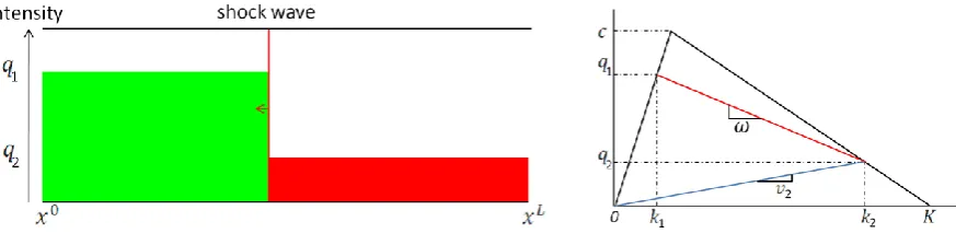
Figure 6. Example of a backward shock wave, with its associated fundamental diagram.

The height of the colored parts indicate the intensity of the flow. The green part indicates free flow conditions (traffic state 1) and the red part indicates congested conditions (traffic state 2), the speed of the traffic will be lower there. Suppose the change of traffic states is initiated at time at location . The shock wave reaches location a certain time later, say at time . The difference in number of vehicles on the link between the moment that the shock wave is initiated and the moment it reaches the other link end can be found by:

Alternatively, this number can be found through the change in flow rates:

Since and the shock wave travels the distance in time , the speed of the shock wave is found as follows:

(

8

)

This speed is also found by determining the slope of the line between the two points on the fundamental diagram (see Figure 6). In this example is negative, because the shock wave travels against the direction of the traffic.

(31)

[image:31.595.73.528.80.246.2]

25

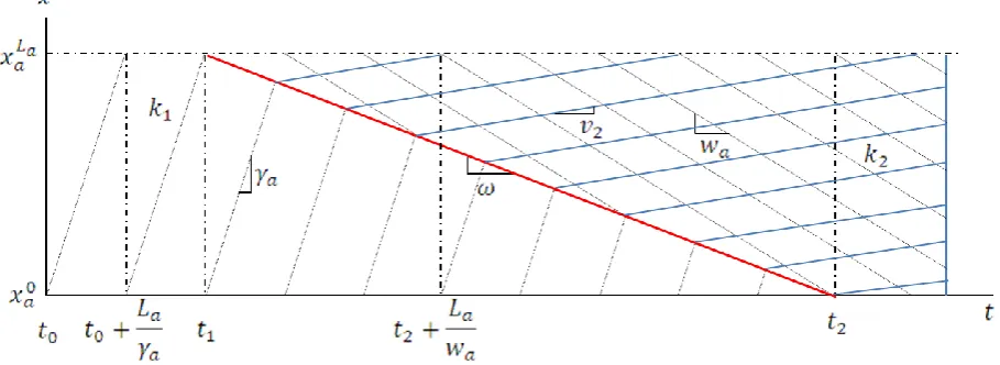
Figure 7. Example of a plane with a shock wave as in Figure 6.

Note that it is assumed that a transition from one traffic state to another does not take time, which implies that vehicles do not accelerate or decelerate. Vehicles make a jump in their driving speed. This assumption simplifies the model greatly, and since the purpose is to model the first order traffic flow and not single vehicles, it is accepted.

There can be many shock waves on the links in a network. Each time a shock wave reaches a link end, it results in new shock waves in the other links connected to this node. By keeping track of all the shock waves in the network, the situation of the traffic flows and densities on the links in the network after a certain time period, for instance one hour, can be calculated.

The Link Transmission Model does model the traffic flows according to the shock waves in the network. However, by using Newell’s simplified theory of kinematic waves (see next section), the LTM only needs to keep track of the cumulative number of vehicles that have entered and left each link, and explicitly keeping track of all the shock waves is no longer needed.

3.5.

Newell’s simplified theory of kinematic waves

As explained before, when using a triangular shaped fundamental diagram, a traffic state can travel through a link with just two possible wave speeds. A traffic state within free flow conditions travels from the upstream boundary (beginning) of link to the downstream boundary (end) of the link with free flow speed . A congested traffic state travels from the downstream boundary of link to the upstream boundary with speed ( is negative, so it travels against the direction of traffic). See also the plane of Figure 7.

A free flow traffic state traveling from the upstream link end following a free flow traffic wave reaches the end of the link time units later, if it does not intersect with another state. Because vehicle trajectories coincide with traffic waves within free flow conditions, the change in cumulative vehicle numbers is zero:

(32)

26

(cumulative outflow). So, when the link is in free flow conditions (when the density is smaller than the critical density, i.e. no congestion), the cumulative number of vehicles that have left the link is equal to the cumulative number of vehicles that have entered the link time units earlier:

(

9

)

[image:32.595.95.348.579.772.2]

In Figure 10 the graph of the cumulative vehicle numbers within free flow conditions is shown, with inflow rate .

Figure 8. Cumulative vehicle numbers within free flow conditions.

A congested traffic state traveling from the downstream link end following a congested traffic wave reaches the beginning of the link time units later, if it does not intersect with another state. With Green’s Theorem (1828) it can be shown that the change in cumulative vehicle numbers is , where is the jam density of link (see also Yperman (2007)). Here is a straight line in the

plane between the points and along which and are constant; both

points represent the same congested traffic state .

(33)

27

The last step is found using the fundamental diagram (see Figure 5a): holds for a congested traffic state , which yields . So, within congested conditions, the cumulative number of vehicles that entered the link at time is equal to the cumulative number of vehicles that have left the link time units earlier plus :

(

10

)

[image:33.595.88.494.284.499.2]

Suppose that as in Figure 7, there is a traffic flow rate of on a link. At time the outflow capacity of the link is reduced to . This will result in congestion on the link, because the current traffic flow rate in the link is . Therefore, from time the graph of the cumulative outflow will have slope , and from time the cumulative inflow will also have slope , with more vehicles (see Figure 9).

Figure 9. Cumulative vehicle numbers within congested conditions.

This results in a double valued solution for the cumulative inflow and outflow, by Figure 8 and Figure 9. The unique solution is achieved by taking the lower envelop of this double valued solution (see Figure 10). Note that in the unique solution the inflow rate changes at time from to , just as found in Figure 7. This solution is found without explicitly calculating the shock wave. This approach works even with multiple shock waves on a link.

(34)

[image:34.595.103.414.80.290.2]

28

Figure 10. The lower envelop of the double valued solution of Figure 8 and Figure 9.

Lemma

Consider a link with traffic state on the whole link. At time the outflow rate changes to

, with corresponding (congested) density . Calculating the arrival time of the shock wave explicitly through the shock wave speed yields the same result as calculating it via Newell’s simplified theory of kinematic waves.

Proof

1. Explicit shock wave arrival time. Following equation (8), the shock wave travels with speed

, so it reaches the upstream link end time units after ( is negative):

2. Newell’s simplified theory of kinematic waves. The arrival time of the shock wave can be calculated following the approach derived from Newell’s simplified theory of kinematic waves. The change in the inflow rate is caused by the arrival of the shock wave at the upstream link end. So, equals the time at which the graph of the cumulative inflow from Figure 10 changes direction, i.e. the time that the graph of the cumulative inflow from Figure 8 crosses the graph of the cumulative inflow from Figure 9:

The cumulative inflow at time of Figure 8 is simply . The cumulative inflow at time of Figure 9 is determined in three parts. Until the cumulative outflow is , then a step of is taken towards the cumulative inflow. Then there is another time of inflow rate . This yields:

(35)

29 Since and it follows that:

Furthermore, since from the fundamental diagram it is known that , it follows that , so:

Since , this is the same result as above.

Kinematic wave theory is described in more detail by e.g. Daganzo (1997) and Newell (1993).

3.6.

Formulation of the Link Transmission Model

Yperman uses equations (9) and (10) in his formulation of sending and receiving flows. In the following, the Link Transmission Model (LTM) by Yperman (2007) is described.

Input for the LTM:

- Network including for each link :

o link capacity (vehicles/hour)

o link length (km)

o jam density, density at which flow is no longer possible (vehicles/km)

o forward (free flow) wave speed (km/hour)

o backward (congested) wave speed (km/hour)

- The fundamental diagram of link , determined by the parameters , and (see Figure 5a). follows from these parameters by .

- : Set of used routes (or paths)

- : Path flow rates for each path at time , the traffic flow per hour assigned to that path (vehicles/hour). Since LTM is a dynamic model, path flows can change over time.

(36)

30

- , the fixed time step in the algorithm. should be smaller than the smallest link travel time. This requirement is known as the Courant-Friedrichs-Lewy (CFL) condition:

To indicate that two links are connected to each other, or more precisely that the downstream end of link is connected to the same node as the upstream end of link , the notation is used.

Variables for the LTM:

The cumulative number of vehicles that have entered link at time .

The cumulative number of vehicles that have left link at time .

The sending flow of link at time (maximum number of vehicles that could leave the downstream end of this link during , if this link end were connected to a traffic reservoir with an infinite capacity).

The directional sending flow from link to link at time , the part of

that wants to go to link . It is assumed that .

The receiving flow of link at time (maximum number of vehicles that could enter the upstream end of this link during , if a traffic reservoir with an infinite traffic demand were connected to this link end).

The transition flow of link to link at time (number of vehicles that are

actually transferred from link to link during ). It is assumed that

.

The LTM basically consists of two parts, the link model and the node model. In the link model the traffic is propagated through the links of the network by determining the sending and receiving flows of each link. The sending and receiving flows indicate the amount of vehicles that are willing to exit and able to enter a certain link, respectively. In the node model, the transition flows are determined.

The sending flow of link at time is the maximum amount of vehicles that could leave the downstream end of this link during , if there are no capacity constraints downstream this link. This means there are free flow conditions in the link. The upper bound for the sending flow is the difference in cumulative outflows at time and , where can be obtained using equation (9) on page 26:

(

11

)

The sending flow is also constrained by the capacity of the link:

(37)

31

So, the sending flow is the maximum flow taking into account equations

(

11

)

and

(

12):

(

13

)

The receiving flow of link at time is the maximum amount of vehicles that could enter the upstream end of this link during , if there is infinite traffic willing to enter this link. This means that the inflow is only constrained by the downstream link end, in case of congestion. The upper bound for the receiving flow is the difference in cumulative inflows at time and , where can be obtained using equation (10) on page 27:

(

14

)

The receiving flow is also constrained by the capacity of the link:

(

15

)

So, the receiving flow is the maximum flow taking into account equations (14) and (15):

(

16

)

In the node model, the transition flows are determined. The transition flows indicate which part of the sending and receiving flows can actually be sent and received, given the situation at that node.

(

17

)

In this node model, the outflow of all incoming links of a node will be reduced if there is a capacity problem at that node. The total flow that want to flow to a outgoing link is the sum of the directional sending flows . However, at most there can flow as much as the receiving flow

to this link. The link with the smallest ratio between the receiving flow and the sum of the directional sending flows determines the factor of the sending flows is allowed to go to the next link at this node.

(38)

32

d e

a 900 0

b 600 1200

[image:38.595.74.454.70.177.2]

c 0 1200

Figure 11. Example of a node with a capacity problem. Table 3. Directional sending flows for the junction of Figure 11.

Because there is a flow of 2400 vehicles per hour that wants to go to link , there is a capacity problem. Following the node model, the transition flows are determined by taking the directional sending flows and multiplying this with the smallest ratio at this node, which is 2000/2400. So, the transition flows are as follows: 750, 500, 1000. Note that even the

outflow from link to link is decreased, while there is no flow from to . However, in this node model it is assumed that when an intersection is congested, all traffic streams are influenced with the same factor.

This node model is chosen for its simplicity, as the formulation is very straightforward. In the paper by Tampère e.a. (2011) this node model is criticized. They show with a numerical example that the total flow over the node with respect to the sending flows is not always maximized. Furthermore, the invariance principle may be violated, which means that a situation can arise in which a queue alternatively grows and dissolves while the boundary conditions (i.e. inflows of the incoming links, outflows of the outgoing links) are constant. The impact of this flaw is not clear and further research on this subject is needed.

A different node model formulation could be implemented in the link transmission model as long as it is applicable to a general intersection, it uses sending- and receiving flows, and the conservation of vehicles and the conversation of turn fractions is guaranteed. Obviously, the flows also need to be non-negative and the demand and supply constraints must be satisfied. The conservation of turn fractions means that the fraction of the sending flow to a certain link is equal to the fraction of the actual flow to that link:

(

18

)

If there is FIFO (first in first out) behavior on the link this requirement is automatically satisfied.

The following sets are used in the algorithm:

(39)

33

The algorithm of the original LTM is as follows. For details, see Yperman (2007).

For each time interval : For each node :

1. For each determine the sending flow using (13), and for each determine the receiving flow using (16).

2. Determine the transition flows from link to link using (17) for all , .

3. Update cumulative vehicle numbers:

3.7.

The stationary Link Transmission Model using flow rates

[image:39.595.92.393.535.732.2]

In the rest of this thesis, it is assumed that the traffic demand is stationary, as in a static traffic assignment model. In this way it is possible to derive the static variant of the LTM. This means that during the whole studied time period the Origin-Destination (OD) demand matrix remains the same, so there is a constant inflow rate onto the first link of each path. This is a static approximation or average of the dynamic demand during a certain time period. In Figure 12 an example of the dynamic demand on a link during the morning peak hours is shown. The stationary approximation will be somewhere between the top and the bottom of the peak. The best way to choose the approximation is not within the scope of this thesis; it is assumed that the stationary demand is given.

(40)

34

Because the OD demand is constant, also the assigned path flows achieved from the route choice model are constant. So, the inflow rate (or intensity) of each first link of all routes is constant. However, because of congestion and spillback effects, this is not true for all links in general. In the following, the sending and receiving flows will be defined in vehicles per hour, at a certain time, instead of a number of vehicles in a certain time interval. Thus, they become sending and receiving flow rates, and also in- and outflow rates. The sending- and receiving flow rates of a node can only change when an (implicit) shock wave reaches this node, for instance when a queue has filled the whole link and is about to spill back. These moments when there is a change in traffic states at a node are called events.

[image:40.595.86.515.355.559.2]

The formulas from the original Link Transmission Model are derived for the stationary case. The event times can be calculated, without iterating for each time step. The time that the next sending or receiving flow rate changes can be determined immediately, instead of calculating the sending and receiving flows for each time step . In Figure 13 an example of the cumulative in- and outflows is gi