A modelling framework for evaluation of the hydrological impacts of nature based approaches to flood risk management, with application to in channel interventions across a 29 km2 scale catchment in the United Kingdom

A modelling framework for evaluation of the hydrological

impacts of nature-based approaches to flood risk

management, with application to in-channel

interventions across a 29km² scale catchment in the

United Kingdom

Peter Metcalfe

, Keith Beven

, Barry Hankin

and Rob Lamb

Lancaster Environment Centre, Lancaster University, Lancaster, LA14YQ, U.K. 2

Department of Earth Sciences, Uppsala University, Uppsala 75263, Sweden 3

JBA Consulting, Sankey Street, Warrington, Cheshire WA1 1NN, U.K. 4

JBA Trust, South Barn, Broughton Hall, Skipton, North Yorkshire, BD23 3AE, U.K.

Abstract

Nature-based approaches to flood risk management are increasing in popularity. Evidence for the effectiveness at the catchment scale of such spatially-distributed, upstream measures is inconclusive, however. It also remains an open question whether, under certain conditions, the individual impacts of a collection of flood mitigation interventions could combine to produce a detrimental effect on run-off response.

A modelling framework is presented for evaluation of the impacts of hillslope and in-channel natural flood management interventions. It couples an existing semi-distributed hydrological model with a new, spatially-explicit, hydraulic channel network routing model.

The model is applied to assess a potential flood mitigation scheme in an agricultural

catchment in North Yorkshire, U.K., comprising various configurations of a single variety of in-channel feature. The hydrological model is used to generate subsurface and surface fluxes for a flood event in 2012. The network routing model is then applied to evaluate the response to the addition of up to 59 features. Additional channel and floodplain storage of

*

*

approximately 70,000m³ is seen with a reduction of around 11% in peak discharge. While this might be sufficient to reduce flooding in moderate events, it is inadequate to prevent flooding in the double peaked storm of the magnitude that caused damage within the

catchment in 2012. Some strategies using features specific to this catchment are suggested in order to improve the attenuation that could be achieved by applying a nature-based approach. Keywords: Natural Flood Risk Management, flood hydraulics, semi-distributed

hydrological models, nature-based solutions

1

Introduction

Since the Second World War more intensive agricultural practices, improved field drainage and changes to land management in the U.K. have led to a significant decrease in many catchments' capacity to retain storm run-off (Wheater et al., 2008; Wheater & Evans, 2009). It has been suggested that this has contributed to the occurrence and severity of flooding downstream of such catchments (O'Connell et al., 2007).

In the period 1980 to 2010 there were 563 individual flood events across 37 European countries, and between 1998 and 2013 flooding caused damage estimated at €54 billion (EEA, 2016). The European Floods Directive (EU 2007), was implemented in November 2007 and requires member states to evaluate the extent and risk of flooding and to take action to mitigate those risks. Amongst other recommendations it emphasises the need for “natural water retention” for flood risk mitigation.

The Pitt Review (Pitt, 2008) that followed extensive floods in England in 2007 contained a recommendation to better “work with natural processes”. The U.K. Environment Agency and other bodies with interests in flood management responded positively to the Review's

In the years since these pieces of legislation were enacted flood mitigation approaches known variously as Natural Flood (Risk) Management (NFM/NFRM), Natural Water Retention Measures (NWRMs, see http://www.nwrm.eu), Nature-based Solutions (NBS), or Working With Natural Processes (WwNP) have gained popularity across Europe. They aim to increase interception and infiltration, slow overland and channel flows and add catchment storage by introducing changes to land use and surface roughness and networks of "soft" engineered features constructed mainly from natural and immediately sourced materials (SEPA, 2012; Quinn et al., 2013). The principle is to restore and improve the catchment’s natural ability to retain storm run-off and to release it slowly, leading to attenuation of downstream flood peaks, whilst retaining or enhancing its ecosystem services (Barber & Quinn, 2012; Maclean et al., 2013).

The Floods Directive is envisaged to be implemented in coordination with the Water

Framework Directive (WFD; EU 2000), which requires member states to implement river

basin management plans that ensure their good ecological and chemical status. It is

recognised that nature-based approaches to river basin flood-risk management may also

target the objectives of the WFD (Wharton & Gilvear, 2007; EEA, 2016).

Nature-based approaches, in contrast, include such techniques as afforestation of hill slopes to increase permeability and downslope transmissivity and so reduce saturated surface run-off andshelterbelts to intercept such flows (Wheater et al., 2008). Tree cover also reduces

effective precipitation input through increased canopy interception and evaporation losses. Bosch and Hewlett (1982) reviewed 94 international studies and concluded that, on average, water yield reduced by between 10 and 40mm for every 10% of catchment reforested, evergreens providing the most effect.

Introduction to the channel of wooden screens or barriers, engineered log-jams (ELJs) or large woody debris (LWD) adds friction and reduces flow velocities (Thomas & Nisbet, 2012; Quinn et al., 2013; Dixon et al., 2016).One significant impact of such in-channel interventions is to create a backwater effect (Quinn et al., 2013),. This may lead to reconnection of the flood plain with the channel at storm flows, and the effect can be substantially enhanced if combined with riparian tree-planting to increase flood plain roughness (Thomas & Nisbet, 2007; Nisbet & Thomas, 2008).

Careful positioning of features such as low earth bunds can disconnect fast overland flow pathways from the channel (Quinn et al., 2013). Offline storage areas can also be used to retain flood water diverted from the channel (Nicholson et al., 2012). Typical capacities are in the range of 200m³ to 1000m³ (Quinn et al., 2013), which means they are unlikely to become subject to the Flood and Water Management Act.

achieved by diverting flood discharge into a pond with a capacity of 27,000 m³. Thomas and Nisbet (2012) estimated a reduction in flow velocities of up 2.1 m/s achieved through the restoration of five woody debris dams in a 0.5 km reach and a 15 minute retardation in the downstream flood peak. Thomas and Nisbet (2007) simulated flood flows thorough new riparian woodland along a 2.2km reach and demonstrated a best case 50% reduction in velocity and delay of 140 minutes in the time to peak.

Despite these localised studies, there remains a need for a modelling approach that can assess the impacts of NFM on realistic catchment scales and the interactions between individual interventions and subcatchments. The effectiveness of riparian measures for flood risk mitigation is considered to be due primarily to desynchronisation of subcatchment flood peaks (Thomas & Nisbet, 2007; Nisbet & Thomas, 2008; Dixon et al., 2016). Dixon et al. (2016) estimated a 19% potential reduction in peak flows, mainly due to this effect,

downstream of a catchment in which 20-40% of the area had been reforested. There remains uncertainty whether the effects of interventions within individual subcatchments could in fact combine to synchronise previously asynchronous peaks (Blanc et al., 2012). The effects of overflow, or even cascading failure, of in-channel structures could also have a detrimental effect on the response (Nicholson et al., 2012).

The study applies the model to evaluate the impact on storm run-off response of a small, intensively cultivated catchment to emplacement of various configurations of in-channel features. A single variety of such feature will be investigated in this paper. We will however discuss how the model could be used to evaluate the impacts of other types of feature and hillslope interventions including enhanced flood plain roughness and hydrological alterations introduced by land use change such as afforestation.

2

Modelling approach

A fully-distributed representation of a realistic catchment and of the processes affected by NFM measures would be both practically and computationally infeasible. In our approach the spatial complexity of the problem is significantly reduced by first applying a semi-distributed hydrological model to simulate hillslope run-off into the channel network. This aggregates similar areas together and treats these as single units within the simulation. Broad-scale measures such as tree-planting and more localised, but greater than grid-scale, features such as run-off detention areas can be included as discrete units in the aggregation. Modifications to those units' parameters and structure to reflect changes introduced when the measures are applied will allow examination of their effects on the response, both at the scale of the unit or on the catchment as a whole.

Thus the hybrid model can not only handle wider interventions whose effects become

noticeable only when applied on the regional scale, but can include sufficient spatial detail to capture features that have greatest impact locally.

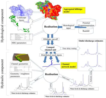
The modelling approach is shown in Figure 1. Due to space limitations full details of the schemes are given in the Electronic Supplement included with the paper.

Figure 1. Overview of the coupled hydrological hillslope- hydraulic network routing modelling

2.1 Hillslope run-off component

Hillslope run-off into the channel network is estimated using the semi-distributed

hydrological model Dynamic TOPMODEL. Details of the principles and use of Dynamic TOPMODEL are given in Beven and Freer (2001) and Metcalfe et al. (2015). The

implementation used in this study is that by Metcalfe et al., (2016), which employs the open-source R language and environment and is freely available from the Comprehensive R Archive Network (CRAN) archive (https://cran.r-project.org/).

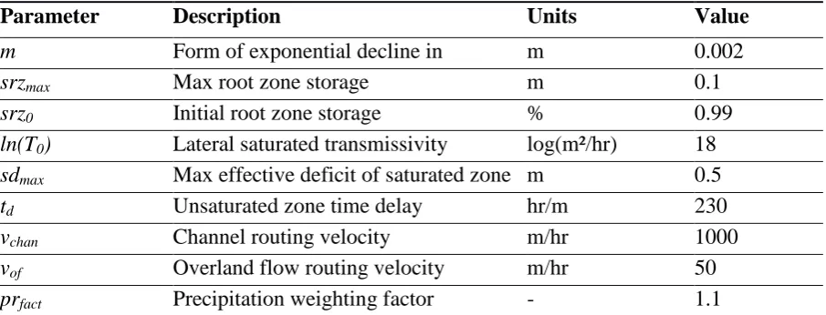
The model groups the catchment into hydrological response units (HRUs) according to landscape characteristics such as topography, land cover or soil type. These units are not necessarily spatially contiguous but they and their time-varying states, averaged over their areas, may be mapped back into space. Each unit is treated as a separate store, the downslope discharge out of which is determined by a suitable storage-discharge relationship. Subsurface flows between the units are distributed according to a flow distribution matrix W estimated from surface slopes used as proxies for the direction of maximum hydraulic gradient. This, along with the units’ storage-discharge relationships, leads to a kinematic wave formulation for downslope flow out of each unit, with a fixed wave speed characteristic to it and its parameters. The hydrological component has relatively few parameters (see Table 1), making the simple to configure and run and allows rapid identification of behavioural model

Table 1. Dynamic TOPMODEL parameters (values are those calibrated against November 2012 storm event, or defaults if not included in calibration)

Parameter Description Units Value

m Form of exponential decline in conductivity

m 0.002

srzmax Max root zone storage m 0.1

srz0 Initial root zone storage % 0.99

ln(T0) Lateral saturated transmissivity log(m²/hr) 18

sdmax Max effective deficit of saturated zone m 0.5

td Unsaturated zone time delay hr/m 230

vchan Channel routing velocity m/hr 1000

vof Overland flow routing velocity m/hr 50

prfact Precipitation weighting factor - 1.1

Saturated excess overland flow is routed to the channel downslope through the HRUs using a surface flow distribution matrix Wof similar to that applied to the subsurface, and the mean

overland flow wave velocity parameter vof ([L]/[T]) whose value can be specified separately

for each unit. The effects of introducing surface roughness to slow saturated overland flow, for example through afforestation, can be approximated by changing the value of vof in the

appropriate unit. To the simulate behaviour of features to intercept overland flow the appropriate elements of Wof can be changed to restrict the downslope drainage out of areas

associated with those features.

The flow distribution matrices are also applied to route hillslope subsurface and surface run-off to the channel, represented as a single lumped unit. An estimate for discharge at the catchment outlet is obtained at each time step by routing the channel input in that interval using a time delay histogram derived from the network flow distances. A fixed channel wave velocity vchan ([L]/[T]) is applied throughout the network.

2.2 Channel routing

the channel with the flood plain. A spatially-explicit, 1D hydraulic channel routing scheme has therefore been implemented.

There exist numerous hydraulic models that allow detailed routing of channel discharge. The model employed by Thomas and Nisbet (2007), for example, is HEC-RAS (Brunner, 1995). This solves the steady state Energy Equation or St Venant unsteady flow equations through successive channels sections. It models the effect of a structure impinging the channel such a bridge as a head loss component additional to friction and contraction / expansion losses. Addition of features and specifications of channel profiles and reaches with these detailed modelling packages is, however, a complex task, and not amenable to automation or rapid modification and calibration. The structures that can be evaluated are generally limited to those implemented by the software, and may not correspond to those we may wish to evaluate as part of an NFM scheme.

Our simpler routing model allows rapid specification of a channel network using spatial vector data and parametric channel and overbank geometries. It enables programmatic definition of in-channel features and their insertion at arbitrary locations across the network. Given suitable constraints on the degrees of freedom allowed in their definition, it can be used to calibrate channel and overbank geometries and roughness. The use of simplified, but realistic, channel geometries allows our model to be run quickly and cheaply where detailed morphological data are not available.

flow. It is however generally adequate for flood routing problems where only predictions of discharges and water levels are required (Knight, 2005).

A separate roughness coefficient may be applied to channel and overbank areas. The effect of introducing roughness to the floodplain to slow overbanked flow can therefore be

investigated by altering the coefficient applied to the overbank component, albeit there may be variations in the effective roughness due to hydrodynamic effects of flow around obstacles such as fallen trees (Thomas & Nisbet, 2007).

In the solution scheme each river reach is divided into approximately equally-sized sub-reaches. At each time step a system of differential equations for sub-reach storages through every reach in the channel network is solved using an iterative, upwinded implicit numerical scheme (described in the Electronic Supplement). Boundary conditions at the upstream inlet to each reach are determined from a channel distribution matrix calculated from the detailed river network. Total discharge between successive sub-reaches Q is then calculated according to the common Manning Equation for open channel flow

n S AR =

Q 0

3 2

(1)

where S0 is the local bed slope, n the Manning roughness, R the hydraulic radius from the

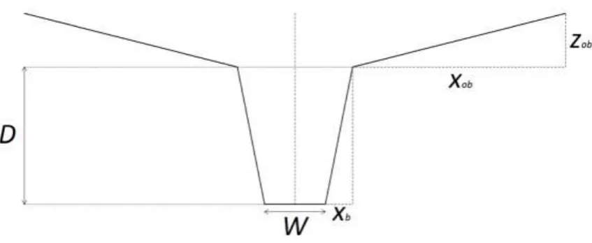
Åkesson et al. (2015) demonstrated that for flood discharge prediction, routing and hydraulic model performance may be more important than channel morphology. Thus by default a simple channel geometry is used in the network routing model. This is a trapezoidal channel section with gently sloped straight floodplain areas extending indefinitely on either side. Such geometries can be parametrised by the channel base width w, the bank slopes sb, floodplain

gradient sob and bank-full level, D (see Figure 2).

The input supplied by the hillslope run-off component to its lumped channel unit is distributed between the reaches according to their length and relative upslope areas. This provides a lateral recharge term for each reach, applied uniformly along its length. The solution scheme outputs, for each time step in a simulation, water levels, flow areas and total discharges through those areas at the mid-point of every sub-reach in the network.

2.3 Representation of in-channel features

effect of an NFM intervention comprising a configuration of in-channel features can be evaluated.

A feature such as weir or barrier may be used that introduces a hydraulic jump. In this case associated energy loss must be taken into account in the relationship. The feature, jump and return to subcritical flow should also be completely contained within a sub-reach. A suitable discharge function, such as a Weir-type equation, can be defined to deal with situations where the feature is overtopped.

Suggested stage-discharge and overflow relationships for some channel features are presented in the Electronic Supplement. Although the geometries considered are highly simplified, Hailemariam et al. (2014) demonstrated that similar idealisations performed adequately against observed data within a simulation of a flood event in a low-lying agricultural catchment in the Netherlands.

3

Study area

(Nicholson et al., 2012). There are few areas of woodland in Brompton, which largely precludes the use of low-cost, locally-sourced woody debris dams employed in the wooded riparian area at Belford (Wilkinson et al., 2010, Nicholson et al., 2012).

The Belford scheme was determined to require at least 20,000 m³ of detention storage within the 5.7 km² catchment area (Nicholson et al., 2012). Brompton is approximately 5 times the plan area of Belford and the storage requirements of an effective scheme will be

commensurately greater. Quinn et al. (2013) consider that an areal contribution of 1 to 10% would be required to add sufficient storage to significantly attenuate the storm hydrograph. Given arable land prices of up to £18000/ha (RICS, 2016) dedicated artificial storage area could be prohibitively expensive. To avoid this, Quinn et al.. (2013) suggest placing features within the channel or in areas of marginal land in steep-sided banking around it. Storage areas will come into operation comparatively rarely and a complementary approach would be to compensate landowners for damage due to periods of inundation. Guidance is available on appropriate rates for various grades of agricultural land subject to different drainage conditions. For example, a week-long flood is estimated to cause damage of £650/ha to extensive arable under good drainage (Penning-Rowsell, 2013).

In contrast to the largely natural channels within Belford, the Brompton network is heavily modified. There are many enlarged and artificial ditches increasing land-channel

connectivity; density is 1203m per km² and there is evidence of extensive and well-maintained subsurface field drainage that connects directly to this ditch network.

3.1 Available data

detailed river network (DRN) obtained from the EDINA DigiMap service was “burnt” into the DEM to a maximum depth of 2m, with a small graduated buffer to impose a consistent hydraulic gradient and flow direction within the channels. Thirty-five river reaches were identified with a median length of 674m.

Hourly rainfall data for nearby weather stations were obtained from the BADC MIDAS repository (Met Office, 2006). The nearest station is at Leeming, about 10km to the SW and at a similar elevation; there is also a gauge at Topcliffe, 17km south of the catchment (see Figure 3b). Using the evapotranspiration module provided with the Dynamic TOPMODEL package, a time series of potential evapotranspiration was generated to give a total actual roughly equivalent to a typical yearly water balance of 230mm.

There is a single gauge at the catchment outlet in Water End, recording stage data at 15-minute intervals. Data for the period 2002-2013 were obtained from the U.K. Environment Agency.

Given the uncertainty introduced by the simplified DRN vector data in determining accurate elevations for channel cells, it was felt that the simplicity of applying an overall bed slope for the entire network would more than compensate for the possible improvements in model accuracy from using a slope calculated for each reach. A value was therefore estimated from the elevation range of DEM cells containing the main channel of Ing and Brompton Becks divided by its total length.

3.2 Field drainage

Subsurface field drainage discharging directly into the channels is apparent in many areas of the catchment. They are mostly less than a metre below the surface, constructed from clay, metal or terracotta and up to 30cm in diameter. According to local farmers some date from the late 19th Century and others were installed as a result of subsidies for field drainage in the 1980s; recent work in the NW of the catchment has used plastic piping of a smaller diameter. Dynamic TOPMODEL by default utilises an exponential transmissivity profile. This is parameterised by T0 ([L]²/[T]), the limiting (saturated) transmissivity and m ([L]) a parameter

controlling the decline of conductivity with depth. Such a form is not required and any suitable profile can be used. A discontinuous transmissivity profile was tried to take into account the effect of the additional capacity introduced at the depth where the drains were found. This, however, seemed to only give marginally closer results to observed hydrographs and introduced extra parameters requiring calibration. The effects of the field drainage appeared to be adequately simulated by favouring parameter sets with high T0 to reflect

3.3 Taking account of tunnels beneath the railway line

At (-1.4082, 54.37606) Ing Beck is crossed by the Northallerton–Middleborough railway, which is carried by an embankment around 30m wide (marked as a cross in Figure 3c). The beck flows through an arched concrete-reinforced tunnel within a brick viaduct, with soffit approximately 4m above the channel bed. Guidelines suggest these features to be considered bridges rather than culverts (Ackers et al., 2015).

It was noted that the area immediately upstream of the crossing provides one of the largest areas of marginal riparian land in the catchment. This is probably due to relatively frequent inundation at storm flows resulting from backwater effects introduced by the tunnel. One of the hypothetical measures considered in the following analysis was to close off the tunnel under the railway line with an engineered sluice gate such as those utilised in flood storage basins. An empirical storage-depth relationship was deduced from the elevation data for the riparian area for the reach approaching the tunnel and applied to the representation of that reach in the flow routing scheme. The results of the simulated intervention are presented in Section 5.3.

4

Storm events, September and November 2012

A minor storm on the 22nd with maximum intensity of 3mm/hr apparently saturated the soil but did not flood the village. After a more prolonged rainstorm of the same maximum intensity a larger peak discharge of 11.2 m³/s is seen in the hydrograph on Sunday 25th, but local residents reported water levels just below that which would cause flooding. There was an overnight recession followed by another storm that began in the early hours of the

following day, with rainfall intensity peaking at 4.4mm/hr around 10am. Rated flow through the gauge peaked at 14.0 m³/s around 5pm. A number of houses were flooded on this

occasion. This suggests that for a scheme to prevent flooding in an event of this magnitude it would have to reduce peak flows by the difference in the two maxima, i.e. by approximately 2.8 m³/s, equivalent to a specific run-off of 0.38mm/hr or around 20% of the peak.

4.1 Calibration of hydrological and hydraulic models

Dynamic TOPMODEL was run using a time step of 15 minutes for the double-peaked storm event of 25th – 27th November 2012. Rainfall data from the Leeming AWS (see Figure 3b) were used and applied evenly across the catchment area. Data from Topcliffe showed similar timings and quantities, indicating that this event was a synoptic event typical of winter rainfalls in this area. A small scaling factor was applied to reconcile the water balance

between input rainfall and observed discharges across the event. Dynamic TOPMODEL does allow for individual rainfall inputs and / or scaling factors for individual HRUs within the catchment model. Given the small extent of the catchment, around 6.5 km square, and the nature of the event, however, it was considered that a uniform rainfall input was adequate for the study.

The model parameters shown in Table 1 were calibrated by running through approximately 5000 realisations with parameters selected at random from the ranges given in the table and applying a performance metric (the Nash Sutcliffe Efficiency, NSE ) to the simulated and reconstructed flows at the outlet with a weighting that took into account the amount of saturated overland flow predicted. Simulations with lower amounts of overland flow were favoured with this weighting in order to reflect the subsurface drainage in evidence. Predicted surface and subsurface hillslope run-off a well-fitting simulation were distributed between the reaches of the channel network and applied to the hydraulic channel routing model.

minutes of those observed. Around 1500 realisations were analysed, and the parameters selected are presented in Table 2.

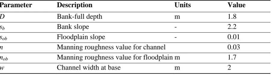
Table 2. Hydraulic model parameters calibrated for November 2012 storm event

Parameter Description Units Value

D Bank-full depth m 1.8

sb Bank slope - 2.2

sob Floodplain slope - 0.01

n Manning roughness value for channel 0.03

nob Manning roughness value for floodplain m 1.7

w Channel width at base m 2

4.2 Selection and sensitivity analysis of flood mitigation interventions

The intensively-farmed nature of the study catchment means there are few options for widespread tree planting and little marginal land in which to site off-line-storage features. In-channel features such as rubble and debris barriers that operate at lower flow stages were also not thought suitable interventions. The Swale and Ure Internal Drain Board (IDB) manages much of the catchment and installation of such features would run counter to the Board’s remit of keeping the channels clear of debris.

Barriers or screens with an opening beneath allow unobstructed flow at normal levels but impinge on storm flows that exceed the underside clearance. They slow these higher flows and introduce channel storage through their backwater effect. These structures are similar to the underflow sluice described in Chow (1959) and their hydraulic characteristics are outlined in the Electronic Supplement. Impermeable, rather than “leaky”, barriers would be most effective in attenuating open channel discharge, although potentially subjected to high hydraulic stresses. The height of the opening could be configured to meet the levels expected for events of a given return period. In practice the geometry of such features is likely to be constrained by compliance with IDB regulations and environmental legislation such as that to allow fish passage (see for example Baudoin et al., 2014).

The storm peak during the simulated November 2012 event arrived about 30 minutes earlier at the outlet of the Winton Beck subcatchment than at the outlet of Ing Beck. Assuming that the rainfall was not a localised convective event, this suggests that measures to slow the combined catchment response should concentrate on Ing Beck as delaying Winton Beck’s response could result in the two peak flows coinciding. There are in addition access issues preventing measures being deployed around Winton Beck.

Features were sized according to the bank-depth of 1.8m with a small upper clearance to allow overflow to drain downstream over the feature rather than into neighbouring fields, as stipulated by the IDB. The barrier tops were set to 1.6m above the base of the channel. As features were added to the network, the functional relationship for the underflow barrier was applied to reaches discharging through a feature, and the routing algorithm run using the modified relationship applied for the corresponding element of the input discharge vector. In addition to discharge, water level and any overflow were recorded for each feature.

5

Results

5.1 Storm simulation

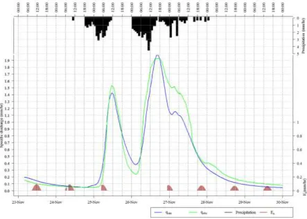
Figure 5 shows the discharge simulated for the storm event of 25th – 27th November using the parameters for the hydrological and hydraulic models given in Table 1 and Table 2,

Reconstructed flows from the observed water levels are also shown. While noting that the observed discharges may be rather uncertain in the way they have been reconstructed (see earlier) the calculated NSE of the simulated discharges was 0.95. The time of the first peak observed at the stage gauge was 11.30am on Sunday 25th November and the corresponding simulated peak was at 11:45am. Time at peak for simulated flows was 16:30 and for the reconstructed flows 17:00 on Monday 26th November. The variation in observed discharges around the storm's peak during the hours of 4pm and 6pm was less than 0.25% of the total. This timing discrepancy was therefore considered to be within the range that could be accounted for by measurement uncertainty.

Figure 5. Simulated hydrograph for a storm event that occurred in November 2012 within the Brompton catchment. Discharges reconstructed from observed water levels shown in green, simulated values in blue. Uncertainty bounds of ±5% could be applied to the reconstructed flows.

5.2 Response tests

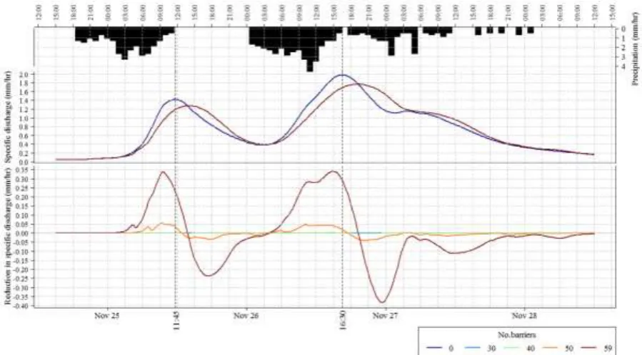
Results for the batches 40, 50 and 59 barriers in the locations shown in Figure 3, using an opening hb=0.3m and maximum height of 1.6m, are summarised in Table 3 and displayed

graphically in Figure 6. This shows the times of peak discharge, difference between the maximum storage in catchment with and without the barriers, and an overall utilisation factor for the scheme util. At any one time the utilisation factor for an individual barrier is the proportion of the potential flow area above the barrier opening that it is intercepting. When the flow is unobstructed the factor is zero, when the water level is above the barrier opening but below its top it is 100%; when the feature starts overflowing the factor starts to falls as the total flow area exceeds the barrier area:

 





Where A0 is the opening area beneath the barrier, Ab is the barrier area above the opening, A

the total channel flow area, h the water level, hb is the barrier opening height and hmax its

Table 3. Summary of catchment response to adding up to 59 barriers, each with a clearance of 30cm, distributed at 300m intervals along the length of Ing Beck and its tributaries. No. barriers Time at peak 26th Nov Delay to peak (hours) Peak discharge (mm/hr) Reduction in peak discharge (mm/hr) % reduction of peak Peak channel storage (m³) Max additional channel storage (m³) Max utilisation (%)

0 16:30 1.98 74846

40 16:30 0 1.98 0.00066 0.03 75891 1045 2.5

50 16:45 0.25 1.96 0.018 0.93 90418 15572 21

59 19:15 2.75 1.77 0.21 10.64 170458 95612 27.4

approximately 0.21 mm/hr or 10.7%. At about 0.35 mm/hr, the largest attenuation in discharge is, however, observed in the rising limbs of both storm peaks. This suggests that the storage capacity of the scheme is filled before both storm peaks. The maximal case delays the arrival of the main storm peak by 2 hours 45 minutes.

The impact increases rapidly as the final 9 barriers are added to the downstream reaches of Brompton Beck, suggesting that most of the effect is due to lower barriers. The

disproportionate effect of these features appears to be due to their effect in diverting flow onto the floodplain, where the much higher roughness reduces flow velocities by a factor of 50. The lowest barrier, for example, diverts overland 45% of the flow from the sub-reach it drains, compared to just 0.3% for the corresponding sub-reach in the unobstructed channel. The scheme seemed to be operating sub-optimally due to under-utilisation of the higher barriers and those downstream reaching capacity and overflowing. In an attempt to improve the impact a second configuration was applied that lowered the clearance of barriers on tributary reaches to just 10cm and raised barriers on the main channel to 80cm. The intention was to improve the utilisation of higher barriers whilst preventing those lower downstream from running out of capacity. The results are shown in Table 4.

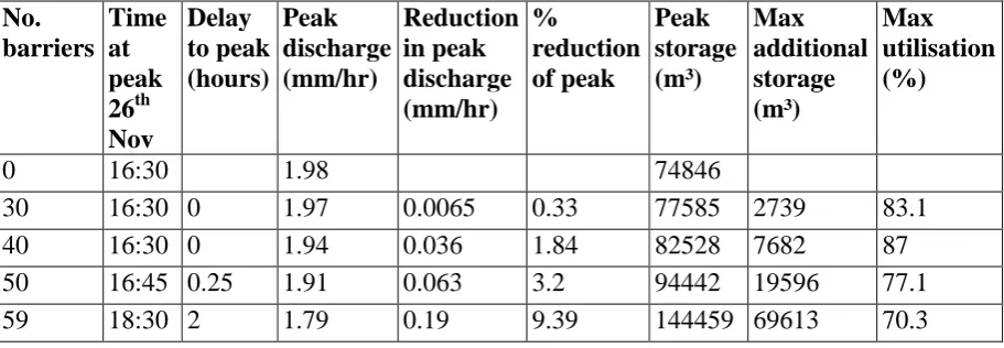
Table 4. Summary of catchment response to adding up to 59 barriers with clearances of 80cm for those on main channel and of 10cm on its tributaries.

No. barriers Time at peak 26th Nov Delay to peak (hours) Peak discharge (mm/hr) Reduction in peak discharge (mm/hr) % reduction of peak Peak storage (m³) Max additional storage (m³) Max utilisation (%)

0 16:30 1.98 74846

30 16:30 0 1.97 0.0065 0.33 77585 2739 83.1

40 16:30 0 1.94 0.036 1.84 82528 7682 87

50 16:45 0.25 1.91 0.063 3.2 94442 19596 77.1

59 18:30 2 1.79 0.19 9.39 144459 69613 70.3

With 40 barriers in place, utilisation reaches a maximum of 87%. In contrast to the first configuration the utilisation then actually starts to decrease as further barriers are added. This is a consequence of the lower barriers operating for shorter periods of time due to their much increased clearance. All of the barriers on the main channel still overflow at some point, however.

Despite the higher utilisation, at 9.4% the peak attenuation in the 40 barrier case is actually lower than for 30 barriers and the delay in the main storm peak is reduced to 2 hours. It appears that some of the features are still draining after the first storm and that the remaining capacity is exhausted more quickly when the next storm arrives. Storage retained from earlier in the storm will contribute to the later storm flows. These barriers “run out” of capacity sooner on the rising limb of the second storm peak than the first, leading to a lower impact at the peak. Brim-full reaches will respond almost as quickly as open channels, leading to a smaller delay in the arrival of the peaks.

5.3 Discussion

Although the first configuration reduced peak flows by almost 11%, it would have not been sufficient to prevent flooding. The overall utilisation for the second configuration was larger but it could not provide any greater capacity to absorb the storm peak. It may be that a further approach with slightly higher upstream and lowered downstream clearances would have avoided this effect, and the simplicity of the routing model allows rapid set up and analysis of this and any other configuration. However, any conclusions drawn are likely to be predicated on the type of event considered. A single-peaked event, such as that commonly used in the assessment of flood scheme performance, might have produced markedly different

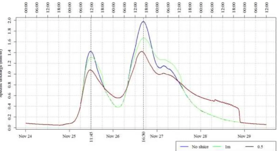
There are other options that would provide significant storage potential sufficient to retain the run-off of the entire event. For example, the railway embankment could be utilised as an “almost” NFM intervention by installing an engineered sluice across the tunnel conveying Ing Beck beneath the line. This could be lowered to reduce the maximum flow rate at storm flows and allow significant quantities of storage to build up behind the embankment during a storm event. The effect of this single intervention was modelled as for the underflow barriers used in the previous analysis but the maximum height hmax was set at 5m. Any overbank flow

generated behind the embankment was intercepted and contributed to the buildup of storage. The response to applying sluice clearances of 1m and 0.5 m is shown in Figure 7 and

Table 5. Summary of catchment response to installation of an underflow sluice across the tunnel conveying Ing Beck under the railway line.

Sluice clearance (m) Time at peak 26th Nov 2012 Delay to peak (hours) Peak discharge (mm/hr) Reduction in peak discharge (mm/hr) % reduction of peak Peak storage (m³) Max additional storage (m³)

16:30 1.98 74846

0.5 15:30 -1 1.42 0.56 28.24 241710 166864

1 16:45 0.25 1.67 0.3 15.4 115400 40554

Applying a 0.5m diameter reduces the second peak by 25% to below the level that would have caused flooding. Peak storage is 168,000m, equivalent over the approximately 72 hour duration of the event to 0.3mm/hr falling across the 8 km² area draining through the viaduct. Maximum water depth of 3m immediately behind the gate was seen some hours before the flood peak and an area of approximately 20 ha flooded to an average depth of about 1m. The area is completely drained by the evening of the 28th, 36 hours after the storm peak. The smallest clearance brings the storm peak forward by one hour. This is simply due to its much Figure 7. Theoretical attenuation of storm hydrograph achieved by installing a sluice across the railway viaduct tunnel and lowering its clearance to 1m and 0.5m. The smallest clearance attenuates the peak to under the discharge that would give rise to flooding at Water End. In this case storage retained behind the viaduct peaks at 168000m³ and is completely drained by the evening of 28th November,

smaller magnitude coinciding with a point midway up the rising limb of the unattenuated case.

It is important to recognise that the scenario involving flow restriction through the tunnel has been included solely as an illustration of the potential to gain significant additional storage capacity through a combination of topography and existing infrastructure. Such opportunities might be available in other catchments. In practice, there are many other considerations relating to the safety and operation of infrastructure, and it is highly unlikely that the owners would allow their asset to be subjected to hydraulic loading in this manner. The additional storage capacity introduced could also lead the intervention to become subject to the

Reservoirs Act, requiring a detailed geotechnical survey, much higher design specifications and significantly greater capital cost.

Similarly, the constraints imposed by the IDB on the channel features, such as the

requirement that they did extend into riparian areas or cause flooding here, clearly limited their effectiveness. Even so, in the modelled scheme downstream barriers appeared to be diverting large quantities of water onto the floodplain: the lowest retained up to 5000m³ in the channel and floodplain immediately upstream, compared to 1500m³ for the same sub-reach for the unobstructed case. This suggests that more relaxed design constraints could allow for a distributed solution that introduced the required storage whilst avoiding the regulatory and cost implications of a large single storage area. If combined with enhancement of riparian roughness to reduce overbank velocities and retain storage on the flood plain, such as was the case in the Ryedale scheme (Nisbet et al., 2011), this could provide significant impacts on storm flows.

screens might be able to withstand the hydrodynamic stresses, but the channel bed and

banking around them would be subject to scour. A regular maintenance regime would have to be established to ensure that the features' performance did not degrade across events and that their structural integrity remained intact.

6

Conclusions and further developments

This study has demonstrated that, with care, a distributed Natural Flood Risk Management scheme could be implemented in the study catchment to reduce peak flows, but that in-channel features alone would not provide sufficient attenuation to prevent recent flood events, at least given realistic constraints in their number and dimensions. It has shown that even an extensive scheme could be substantially underutilised and provide little or no

attenuation to the storm hydrograph. Barriers furthest downstream contribute relatively more attenuation with the attendant risk of failure due to large hydraulic stresses.

A scheme utilising a reduction in the capacity of the railway tunnel feature specific to the catchment could, however, deliver the required response. However this might not be

considered an acceptable solution for other reasons, such as the potential for damage at storm flows. In addition, the volumes involved mean that if a structure of equivalent storage

either unused or overloaded. The available storage capacity may become saturated in

intermediate events and not recover sufficiently quickly in order to provide capacity for later storms.

Much of the attenuation is due to the lower barriers, mainly through their effect of

reconnecting the floodplain with the channel and diverting large quantities of overbanked flow through the rougher riparian area. It is suggested that schemes should concentrate on encouraging this effect using fewer, larger barriers further downstream in preference to many smaller barriers in the upper reaches. This approach, however, would also introduce much greater hydraulic stresses and correspondingly greater rating specifications and maintenance requirements, albeit that this would be reduced due to the fewer structures. The potential of cascading failures should be considered, not least due to the potential for blockage of downstream structures such as tunnels.

The (hypothetical) measures that provided the greatest effect were the throttling of the flow through the railway tunnels and emplacement of barriers downstream to divert water onto the flood plain, both of which would involve the inundation of significant areas of productive agricultural land. This introduces much potential for conflict with land owners and regulatory bodies such as the IDB, whose priorities in terms of channel and run-off management are likely to diverge from those of NFM practitioners. Experience from the Belford scheme where a pilot site was established before the main scheme was begun (Wilkinson et al., 2010), and the stakeholder collaborative approach adopted in Ryedale (Lane et al., 2011) suggest ways that resistance to the adoption of such new approaches to flood risk

management may be overcome.

Acknowledgements

This work has been funded by the JBA Trust (project number W12-1866) and managed by the Centre for Global Eco-innovation (CGE project number 132)

Many thanks to Sue Butler, Jan Hodgson and other members of the Brompton Flood Group for their help, photography and support.

Supporting information

Electronic Supplement 1: Hydraulic channel routing model

Electronic Supplement 2: Hydraulic characteristics of run-off attenuation features

References

Supplementary material can be found in the supporting information included with this paper. Ackers, J., Rickard, C. & Gill, D. (eds) (2015). Fluvial Design Guide. Environment Agency,

Bristol, U.K.

Åkesson, A., Worman, A., & Bottacin-Busolin, A., 2015, Hydraulic response in flooded stream networks, Water Resour. Res., 51, 213–240, doi:10.1002/2014WR016279 Barber, N. J., & Quinn, P. F. 2012. Mitigating diffuse water pollution from agriculture using

soft engineered runoff attenuation features. Area, 44(4), 454-462.

Baudoin, J.M., Burgun, V., Chanseau, M., Larinier, M., Ovidio, M., Sremski, W., Steinbach, P. & Voegtle, B., 2014. Assessing the passage of obstacles by fish. Concepts, design and application. Onema, France.

Bosch, J. M., & Hewlett, J. D. (1982). A review of catchment experiments to determine the effect of vegetation changes on water yield and evapotranspiration. Journal of hydrology, 55(1-4), 3-23.

Brunner, G. W. 1995. HEC-RAS River Analysis System. Hydraulic Reference Manual. Version 1.0. Hydrologic Engineering Center Davis CA.

Beven, K.,& Freer, J., 2001. A Dynamic TOPMODEL. Hydrological Processes,15(10), 1993-2011.

Blanc, J. Wright. G & Arthur S., 2012, Natural Flood Management knowledge system: Part 2 – The effect of NFM features on the desynchronising of flood peaks at a catchment scale. CREW report.

Chow, V., 1959. Open channel hydraulics.

Dixon, S. J., Sear, D. A., Odoni, N. A., Sykes, T., & Lane, S. N. (2016). The effects of river restoration on catchment scale flood risk and flood hydrology. Earth Surface

Processes and Landforms, 41(7), 997-1008.

Environment Agency, 2012. Greater working with natural processes in flood and coastal erosion risk management – a response to Pitt Review Recommendation 27. Environment Agency led working group.

EU, 2000, Directive 2000/60/EC of the European Parliament and of the Council of 23 October 2000 establishing a framework for Community action in the field of water policy, OJ L327, 22.12.2000.

EU, 2007, Directive 2007/60/EC of the European Parliament and of the Council of 23

European Environment Agency, 2016. Flood risks and environmental vulnerability.

Exploring the synergies between floodplain restoration, water policies and thematic policies. EEA Report No 1/2016

Ghimire, S, Wilkinson, M. & Donaldson-Selby, G., 2014. Application of 1D and 2D numerical models for assessing and visualizing effectiveness of natural flood management (NFM) measures. Paper presented at 11th International Conference on Hydroinformatics, New York City, USA. Retrieved 01/12/2015 from

http://www.hic2014.org/proceedings/bitstream/handle/123456789/1399/1391.pdf Hailemariam, F. M., Brandimarte, L., & Dottori, F., 2014. Investigating the influence of

minor hydraulic structures on modeling flood events in lowland areas. Hydrological Processes, 28(4), 1742-1755.

JBA Trust, 2016. "Working with natural processes to reduce flood risk". Retrieved

05/05/2016 from http://www.jbatrust.org/news/working-with-natural-processes-to-reduce-flood-risk

Knight, D., 2005. River flood hydraulics: validation issues in one-dimensional flood routing models. In Knight, D., & Shamseldin, A. (Eds.). River basin modelling for flood risk mitigation. CRC Press.

Lane, S. N., Odoni, N., Landström, C., Whatmore, S. J., Ward, N., & Bradley, S., 2011. Doing flood risk science differently: an experiment in radical scientific

method. Transactions of the Institute of British Geographers, 36(1), 15-36.

Met Office 2006: U.K. Hourly Rainfall Data, Part of the Met Office Integrated Data Archive System (MIDAS). NCAS British Atmospheric Data Centre,

http://catalogue.ceda.ac.U.K./uuid/bbd6916225e7475514e17fdbf11141c1

Metcalfe, P., Beven, K., & Freer, J., 2015. Dynamic TOPMODEL: A new implementation in R and its sensitivity to time and space steps. Environmental Modelling & Software, 72, 155-172.

Metcalfe, P., Beven, K., & Freer, J., 2016. dynatopmodel: Implementation of the Dynamic TOPMODEL Hydrological Model. R package version 1.1.

https://CRAN.R-project.org/package=dynatopmodel

McLean, L., Beevers, L., Pender, G., Haynes, H., & Wilkinson, M., 2013. Variables for Measuring Multiple Benefits and Ecosystem Services. Infrastructure and Environment Scotland 1st Postgraduate Conference.

Nicholson, A. R., Wilkinson, M. E., O'Donnell, G. M., & Quinn, P. F., 2012. Runoff

attenuation features: a sustainable flood mitigation strategy in the Belford catchment, U.K.. Area, 44(4), 463-469.

Nisbet, T.R., Thomas, H., 2008. Restoring floodplain woodland for flood alleviation. Final report for the Department of Environment, Food and Rural Affairs, Project SLD2316. DEFRA, London.

Nisbet, T.R., Marrington, S., Thomas, H., Broadmeadow, S.B. and Valatin, G., 2011.

Slowing the Flow at Pickering. Final report for the Department of Environment, Food and Rural Affairs, Project RMP5455. DEFRA, London.

Penning-Rowsell, E., Priest, S., Parker, D., 2013. Flood and coastal erosion risk management: a manual for economic appraisal. Routledge.

Pitt, M., 2008. The Pitt Review: Learning lessons from the 2007 floods. London: Cabinet Office.

Quinn, P., O’Donnell, G., Nicholson, A., Wilkinson, M., Owen, G., Jonczyk, J., Barber, N., Hardwick, M., Davies, G., 2013. Potential use of Runoff Attenuation Features in small rural catchments for flood mitigation. England: Newcastle University, Environment Agency, Royal Haskoning DHV.

RICS 2016. RICS/RAU Rural Land Market Survey. Accessed 01/12/2015 from

http://www.rics.org/U.K./knowledge/market-analysis/ricsrau-rural-land-market-survey-h2-2013/

Scottish Environment Protection Agency, “Natural Flood Management Position Statement: the role of SEPA in natural flood management”. Accessed 01/12/2015 from

http://www.sepa.org.U.K./flooding.aspx.

Skublics, D., & Rutschmann, P. (2015). Progress in natural flood retention at the Bavarian Danube. Natural Hazards, 75(1), 51-67.

Thomas, H., & Nisbet, T. R., 2007. An assessment of the impact of floodplain woodland on flood flows. Water and Environment Journal, 21(2), 114-126.

Thomas, H. and Nisbet, T.R., 2012. Modelling the hydraulic impact of reintroducing large woody debris into watercourses. Journal of Flood Risk Management 5 (2):164 – 174. Wilkinson, M.E., Quinn, P.F., Welton, P., 2010. Runoff management during the September

2008 floods in the Belford catchment, Northumberland. Journal of Flood Risk Management, 3(4): 285-295.

Wharton, G., & Gilvear, D. J., 2007. River restoration in the U.K.: Meeting the dual needs of the European Union Water Framework Directive and flood defence? International

Journal of River Basin Management, 5(2), 143-154.

Wheater, H., Reynolds, B., McIntyre, N., Marshall, M., Jackson, B., Frogbrook, Z. & Chell, J., 2008. Impacts of upland land management on flood risk: Multi-scale modelling methodology and results from the Pontbren experiment.

7

Electronic Supplement :

7.4 Hydraulic channel routing scheme

The depth-averaged one-dimensional St Venant equations for open-channel flow in a prismatic channel with an arbitrary profile, expressed in terms of flow area A, water level h and total discharge Q through the area, are (see Henderson, 1966; Cunge et al., 1980; Knight, 2006; Beven, 2012 and many others)

𝜕𝐴

𝜕𝑡 +

𝜕𝑄

𝜕𝑥 = 𝑟

(S1)

𝜕𝑄

𝜕𝑡 +

𝜕

𝜕𝑥(𝛽

𝑄2

𝐴) + 𝑔𝐴 (

𝜕ℎ

𝜕𝑥+ 𝑠𝑓− 𝑠0) = 0

(S2)

x is the distance measured in the downstream direction and r the lateral recharge per unit length of the channel. Recharge is the sum of specific subsurface base flow 𝑞𝑏𝑓 and any overland flow 𝑞_𝑜𝑓 and is supplied by the hydrological component described in the main text. The total channel input at each time step is distributed between the reaches according to a weighting matrix derived from the surface topography, similar to that used to route base flows between landscape units in Dynamic TOPMODEL. For reach i the recharge ri is then applied uniformly along its length.

The channel bed slope, assumed constant over the reach is 𝑠0,  is a momentum correction coefficient to account for variation of flow velocity across the flow area, which, in the absence of further information, can be taken as unity. Given these assumptions the mean channel velocity is taken as 𝑉 = 𝑄 𝐴⁄ .

𝑠_𝑓 is the head loss due to friction against the bed per unit length of downstream flow. For uniform flow the friction slope can be approximated using the Manning

𝑠_𝑓= 𝑉|𝑉|𝑛2 𝑅4 3⁄

(S3)

with n the roughness and R the hydraulic radius calculated from the wetted perimeter and flow area. If gradually-varied and subcritical flow is assumed, the first two terms in (S2), representing the temporal and advective acceleration respectively can be neglected, leading to a diffusive wave approximation for open channel flow:

𝜕ℎ

𝜕𝑥+ 𝑠𝑓− 𝑠0 = 0

(S4)

Substituting (S3) into (S4) and rearranging gives an expression for the mean flow velocity. Multiplication by the flow area then leads to an analytical expression for the discharge:

𝑄 =𝐴𝑅

2 3⁄

𝑛 √𝑠0−

𝜕ℎ 𝜕𝑥

(S5)

Given a channel network comprised of M reaches, a numerical scheme is now

constructed as follows in order to solve for channel flows at discrete time steps across a simulation.

In order to reduce the problem from a system of partial differential equations in two independent variables x and t to a coupled system of ordinary differential equations (ODEs) the spatial dimension x is discretised. This is known as the Method of Lines (MOL, see Hamdi et al., 2007). Reach i is subdivided into Ni segments, each of length

∆𝑥𝑖. If the flow out of segment j is Qj, its end point at downstream position 𝑥𝑗 = 𝑗∆𝑥𝑖,

then mass continuity expressed by (S1) is approximated in this segment by 𝑑𝐴

𝑑𝑡|_{𝑥=𝑥𝑗} ≈ 𝑟𝑖 −

(𝑄𝑗− 𝑄𝑗−1)

∆𝑥_𝑖 , 𝑗 = 1, 𝑁𝑖

Water levels hj are calculated at the boundary of all segments using the chosen

channel geometry and the flow area at the current time step. For a rectangular channel of width w the water level is simply 𝐴/𝑤 but any profile may be specified, including

ones where a shallow floodplain is defined. This allows the water surface gradient 𝜕ℎ

𝜕𝑥−𝑠0 to be estimated for the segment. A “downwind” scheme is used so that the effects of afflux behind constrictions and backwater effects at confluences can be propagated upstream, hence

𝜕ℎ 𝜕𝑥|𝑥=𝑥𝑗

≈(ℎ𝑗+1− ℎ𝑗) ∆𝑥𝑖

(S7)

The channel is divided into overbank and in-channel components that may take distinct geometries and roughness values. If the flow remains in channel the appropriate values for the channel may be simply substituted into (S5) in order to obtain the overall discharges. Where water goes overbank the discharges in and out of channel are calculated separately and added to give the overall flow through the subreach. The overbank area is deemed to be that lying above the floodplain; the area above the channel but above the bankfull depth D is allocated to the in-channel flow. In a typical trapezoidal channel this results in the overbank area making a broad-based triangle on each bank with the in-channel component a hexagon. The values for R and

A are calculated in each of the areas and they and the appropriate Manning n and the water surface gradient are substituted into (S5) and summed.

Reaches are defined strictly between the entry points of tributaries. The channel network is formalised as a directed graph whose edges correspond to the channel reaches and the vertices to springs, confluences and the catchment outlet. A flow direction, or adjacency, matrix F is constructed from the graph, describing how flow is routed downstream out of the reaches. Its elements Fij are equal to 1 if reach j flows

into reach i, zero otherwise.

If flows out of all reaches is held in the vector 𝑄𝑜𝑢𝑡 and the upstream inputs (zero for source reaches with no upstream input) by 𝑄₀, then mass and momentum conservation is enforced by setting 𝑄₀ = 𝑭Q_𝑜𝑢𝑡.

In channels with arbitrary profiles mass conservation implies that flow areas, rather than water levels, are additive. That is, if reaches i and j with final flow areas 𝐴_𝑖 and 𝐴_𝑗 converge to form reach k then, assuming no other inputs, the flow area at the first segment of reach k is 𝐴_𝑘 = 𝐴_𝑖 + 𝐴_𝑗. For source reaches 𝐴₀ will be zero. Assuming quasi-steady flow for the duration of the time step, if 𝐴′0 is the vector of flow areas at the start of reaches that have an upstream input, given by the vector 𝐴_𝑜𝑢𝑡, and F’ the adjacency matrix for just those reaches then the upstream flow areas can be estimated as 𝐴′₀ = 𝑭′−𝟏_𝐴

𝑜𝑢𝑡.

The corresponding water level will be calculated according to the relationship for the channel profile applied. This allows the water surface gradient calculated in (S7) to be determined at the end of each reach. At the outlet as there is no downstream reach supplied the water surface gradient is carried through from the previous segment. The resulting system of ∑𝑀 𝑁_𝑖

be lost at longer time intervals and a step of 15 minutes is typically used. We employ the Livermore Solver for Ordinary Differential Equations (lsode, Petzold, 1993) to solve the system. It is open-source compiled FORTRAN optimised for both stiff and non-stiff systems. It automatically employs an implicit backwards Euler scheme in periods of non-linearity and a forward (explicit) approach when flows are more stable. Segment lengths must be chosen that are short enough to determine the flux gradient reasonably accurately but long enough to prevent it being over-estimated and giving rise to numerical instabilities in front of a flood wave. Samuels (1989) suggests a minimum segment length given by the expression ∆𝑥𝑚𝑖𝑛 =0.15𝐷_𝑠

0 ; 50m has been used

in the analysis presented in the main text.

7.5 Representation of in-channel features

Given an appropriate stage-discharge relationship for a particular type of runoff attenuation, such as those presented below, the above scheme may be modified to take into account the effect of adding features with the channels.

Features may be sited within at the end of any subreach, index f, say, within the network. The value for the output discharge, 𝑄𝑓, calculated in (S5) is replaced by the appropriate value calculated from the stage-discharge relationship for the feature. If the feature vertical extent is below the bankfull level then overbank flow is assumed to bypass the feature and is calculated as before. An additional overflow component is added to the in-channel flow through the feature, calculated as a function of the water level above its top. This is typically a weir-type equation (ISO, 1980):

𝑄_{𝑜𝑣𝑒𝑟} = 2

3𝐶w𝑤𝑏√2𝑔(ℎ − ℎ𝑚𝑎𝑥)3/2

where 𝑤_𝑏 is the dam’s width ℎ_𝑚𝑎𝑥 along its top side, its maximum height above the channel bed, and 𝐶_w a weir coefficient, which must be empirically determined. A typical value is 0.68 for a sharp, non-contracted rectangular weir but will differ for other geometries.When the water overtops the feature, additional flow is calculated by its overflow function applied across the top width.

Approximate storage-discharge relationships for typical runoff attenuation features are presented in the following section of this Electronic Supplement. These include bunds, large woody debris (LWD) barriers, underflow ditch barriers or screens and overflow storage basins.

8

Hydraulic characteristics of runoff attenuation features

As previously described, in order to incorporate runoff attenuation features in the routing scheme it is required to specify a stage-discharge relationship appropriate to that structure. For most the downstream water will have some impact on the discharge through the feature. In the routing scheme described in the previous section this is approximated by the level at the start of the time step.

8.6 Bunds

A simple feature to add storage is a small earth dam (also known as a bund) placed across the channel or in an overland flow pathway. In the case of a bund placed in a channel with maximum height hmax above its bed, with the outlet treated as one or

more smooth pipes close to the base each with diameter d<<hmax the discharge may

simply be calculated by consideration of conservation of energy.

For smooth outlet pipe(s) of total cross-sectional area 𝑎_𝑝 the outlet discharge is thus 𝑄 = 𝑎𝑝√2𝑔∆ℎ. For realistic pipes a coefficient in the range 0.5 to 1 could be applied

to account for friction loss.

The above assumes that the water immediately behind the feature is effectively stationary. In practice the approach velocity will affect upstream level, as the velocity head will be translated into potential energy . Equating the upstream and downstream heads:

ℎ₂ = 𝑣12 2𝑔+ ℎ1

(S9)

where 𝑣₁ is the approach velocity, ℎ₁ the water level upstream of the dammed, stationary subreach, and ℎ₂ the water level immediately behind the feature. A typical approach velocity of around 1m/s would therefore result in an additional water depth of around 5cm.

For a dam placed across a rectangular channel of width w filled to a level h the

specific storage ([L]³/[L]) immediately upstream is simply hw. A more realistic profile would be a symmetrical inverted trapezoidal prism. The channel forms its shortest width w, also taken as the width of the base of the dam. The banks to the top of the dam are assumed approximately straight with slope sb. The specific storage per reach

length given a water level h at the upstream edge of a dam feature placed within this profile can be shown to be 𝑠 = ℎ (_𝑠ℎ

𝑏+ 𝑤).This allows the dammed water level ℎ for a

given specific storage s to be calculated as

ℎ =𝑠𝑏

2 (−𝑤 + √𝑤2+

4𝑠 𝑠_𝑏)

(S10)

When the dam is overtopped the weir equation (ISO, 1980) can be used to predict the overflow discharge:

𝑄_{𝑜𝑣𝑒𝑟} = 2

3𝐶w𝑤𝑏√2𝑔(ℎ − ℎ𝑚𝑎𝑥)3/2

(S11)

where 𝑤_𝑏 is the dam’s width, ℎ_𝑚𝑎𝑥 along its top side, its maximum height above the channel bed, and 𝐶w a weir coefficient, which must be empirically determined. A typical value is 0.68 for a sharp, non-contracted rectangular weir but will differ for other geometries.When the water overtops the feature, flow calculated by this function is added to the discharge through the outlet pipe(s) to obtain the total discharge

through the feature.

In practice an earth or wooden bund would be losing water both through infiltration and seepage through its walls. In this case it may be more realistically modelled as a woody debris dam with tightly-spaced members (see 8.8).

8.7 Ditch barriers

Barriers or screens, typically wooden, can be placed across the channel a small

distance above the normal water level. These allow unobstructed drainage at for levels below the top of the barrier opening flows but increasingly impede discharge as the water level rises above this. They are hydraulically similar to underflow sluices (gates) such as those employed in irrigation networks or canals, but in a natural flood management scheme are unlikely to be manually operated.

Consider a horizontal barrier whose top is at a height ℎ_𝑚𝑎𝑥 above the channel bed with a clearance of the underside of the barrier from the channel bed of a and an upstream water level at a particular time of h0. As can be seen from Figure S.1 there is

distance and hydraulic jump the flow returns to subcriticality and the water level recovers. The level of the critical flow section is ℎ₁ and the subcritical downstream, or tailwater, level is h2.

Figure S 1. Definition sketch of underflow barrier (Swamee, 1992)

The modes of operation of the feature are (Swamee, 1992): 1. ℎ₀ < 𝑎 no impediment to flow due to barrier; 2. ℎ₀ ≥ 𝑎 barrier in operation with free discharge;

Error! Reference source not found.The standard depth-discharge relationship for the operational underflow sluice is (Chow, 1959)

𝑄 = 𝐶_𝑑𝑤_𝑏𝑎√2𝑔𝑎 (S12)

where 𝑤_𝑏 is the width of the barrier at its base. This can be seen as analogous with the Torrecelli Equation but with the addition of a energy gain/loss factor 𝐶_𝑑, termed the Coefficient of Discharge. 𝐶_𝑑 incorporates upstream velocity head, friction and energy loss through the hydraulic jump. The development of 𝐶𝑑 with ℎ0 and ℎ2 must be empirically determined.

For the first mode the open-channel routing approach described in the main paper is applied. For the operational barrier with free discharge (mode 2) Swamee (1992) identifies an approximate functional relationship between 𝐶_𝑑 and ℎ₀ through experimental results due to Henry (1950):

𝐶𝑑,𝑓𝑟𝑒𝑒(ℎ0) = 0.611 (

ℎ₀− 𝑎 ℎ0 + 15𝑎)

0.072

He also derives a condition to determine the existence of free discharge

ℎ0 ≥ ℎ𝑡ℎ𝑟𝑒𝑠ℎ(ℎ2) = 0.81. ℎ2( ℎ₂

𝑎) 0.72

He then suggests for submerged discharge (mode 3) the following relationship

𝐶𝑑,𝑠𝑢𝑏(ℎ0, ℎ2) =

𝐶_{𝑑,𝑓𝑟𝑒𝑒}(ℎ0)∆ℎ0.7

(0.32. (ℎ𝑡ℎ𝑟𝑒𝑠ℎ− ℎ0)0.7+ ∆ℎ0.7)

(S13)

where ∆ℎ = ℎ₀ − ℎ₂

Overflow when the feature is overtopped is calculated as for a bund, (S13).

scheme it was found necessary to define a short transitional region for water levels just above the barrier. This is to prevent a discontinuity between discharges in modes 1 and 2 or 3 which prevents the scheme from converging. In the transitional zone the discharge is linearly interpolated between its value in mode 1 immediately below the barrier at in mode 2 at the top of the region. This region could be thought of

corresponding to the regime where the barrier is just impinging the flow, with orifice flow starting to become apparent.

8.8 Large woody Debris (LWD) or “leaky” dams

A barrier comprised of tree trunks, large branches, timber lengths or fallen trees placed across the channel adds a significant resistive component to flow. Unlike the impermeable barriers described in the previous section, where water behind the barrier is treated as being effectively stationary, the velocity through the barrier will be non-negligible and the resistance will be proportional to this velocity. This approximation will become inaccurate with increasing approach velocity and the velocity head attains a similar magnitude to the hydrostatic head. The head loss across the barrier can be estimated by the density and shape of the timber pieces. This structure could be seen as analogous to a trash screen such as those employed to trap debris upstream of structures such as culverts or before the intakes to water treatment works and power plants.

Kirschmer’s equation (Kirschmer, 1926) may be used to estimate the proportion of upstream velocity head lost through the structure. Equating total head upstream and downstream of the barrier allows a head loss coefficient, c, to be calculated ,such that

𝑐 = 𝛽 (𝑠 𝑏)

4 3 ⁄