Management Science
Working Paper 2018:5
Modelling Dairy Supply Chain in West Java
using Agent-Based Simulation
Dhanan Sarwo Utomo, Bhakti Stephan Onggo, Stephen
Eldridge
The Department of Management Science
Lancaster University Management School
Lancaster LA1 4YX
UK
© Dhanan Sarwo Utomo, Bhakti Stephan Onggo, Stephen Eldridge All rights reserved. Short sections of text, not to exceed two paragraphs, may be quoted without explicit permission,
provided that full acknowledgment is given.
Modelling Dairy Supply Chain in West Java using Agent-Based
Simulation
Dhanan Sarwo Utomo1, Bhakti Stephan Onggo2, Stephen Eldridge1
1Department of Management Science, Lancaster University Management School, Lancaster
University, United Kingdom
2Trinity Business School, Trinity College Dublin, The University of Dublin, Republic of
Ireland
Abstract
This working paper describes a process to develop an agent-based simulation of dairy supply
chain in Indonesia. The discussion begins by describing the situation in the case study area.
Then we explain the assumptions used in to develop agent-based simulation in this study. The
simulation experiments show that the agent-based simulation can produce outputs that
resemble the patterns in the real-world data. This paper ends by discussing the conclusions and
plan for further research.
Keywords: Agent-based simulation, dairy supply chain
1. Introduction to the dairy supply chain in Indonesia
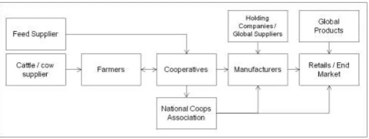
Figure 1 shows the typical dairy supply chain in Indonesia that is composed of many tiers
comprising farmers (producers), cooperatives (collector and handler), milk processing
[image:2.595.114.486.535.675.2]industries (manufactures), retailers and consumers.
Figure 1 Generic structure of dairy supply chain in Indonesia (Daud et al., 2015)
In common with earlier studies (for example Glock (2012)), the number of farmers is large
while the number of milk processing industries. Most farmers are smallholders with low
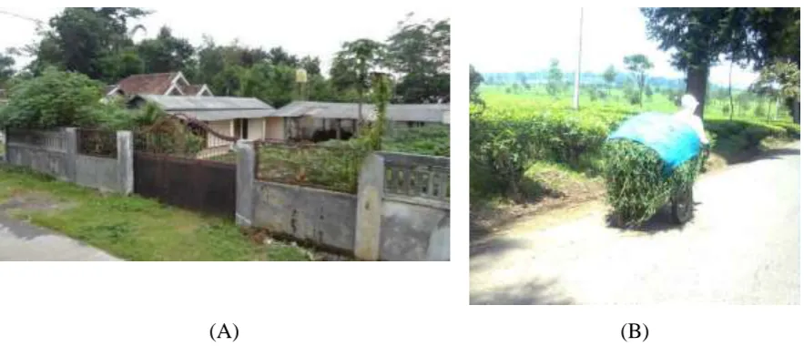
usually, it is only sufficient to build a pen for their cattle. The pens are usually located next to
the farmers’ houses in the middle of residential areas for security reasons. The forage grows
along the road and river banks. It is difficult for the farmers to herd their cattle through the
residential area. Therefore, the forage must be gathered from outside of their village and
transported back using carts or motorcycles. In this sense, forage is a common resource for all
these farmers. When the forage availability is low, the competition between farmers to obtain
forage becomes more intense.
(A) (B)
Figure 2 (A) A cattle pen in the middle of a residential area. (B) A farmer is transporting forage using a cart.
In this supply chain, the milk produced by the farmers is collected and transported to the milk
processors by farmers’ cooperatives. The role of a farmers’ cooperative is important because it
is cheaper for the milk processing industries to buy milk in large quantities and, also, the milk
that is highly perishable must be transported efficiently and refrigerated at all times (Glover et
al., 2014, Manish and Sanjay, 2013), this is prohibitively expensive for the smallholder farmers.
However, the farmer cannot fully control the cooperative’s decisions because the cooperative
also has external investors, shareholders and employs professional managers and workers.
Hence the cooperative works like an independent company with smallholder farmers act as its
suppliers that have little influence on the cooperative’s decisions.
2. The process to model the dairy supply chain in West Java using Agent-Based Simulation
Utomo et al. (2018) suggested that the majority of ABS applications in the agri-food supply
chain focus on one tier namely the producer. Moreover, previous studies were commonly
carried out in high-income countries and involve big farmers. The agent-based simulation in
[image:3.595.78.520.221.411.2]Pangalengan, West Java. Pangalengan is a 27,294.77 ha agricultural and plantation region.
Smallholder dairy businesses have emerged in this region since the 1940s. Nowadays, the dairy
supply chain in this region is one of the biggest in Indonesia hence it is considered to be
representative of other dairy supply chains in the country.
We began developing an ABS dairy supply chain in Pangalengan by gathering the relevant
body of knowledge from previous studies, as suggested by Gilbert (2004). We found two sets
of models relevant to the dairy supply chain in the previous literature. The first set of models
assumes that farmers have a land endowment. They maximise their income by allocating their
land to produce multiple crops. If they decide to produce milk, then they allocate some of their
land to grow the forage. Examples of these models are Happe et al. (2009), Happe et al. (2011),
Marohn et al. (2013), and Quang et al. (2014). The second set of models comprise grazing
models in which the farmers herd their livestock to a common source of forage (i.e., the
rangeland). Examples of these models are Boone et al. (2011), Rasch et al. (2016), Martin et
al. (2016), Rasch et al. (2017). In the case study area, the farmers also mainly rely on their
surrounding environment as a common source of forage. Hence we considered the second set
of models to be more suitable as the foundation of our modelling. The main difference is that
the farmers in our case need to transport forage for their cattle, while the cattle do not move at
all. Forage transportation introduces more production constraints into our modelling such as
labour, working hours and transport capacity.
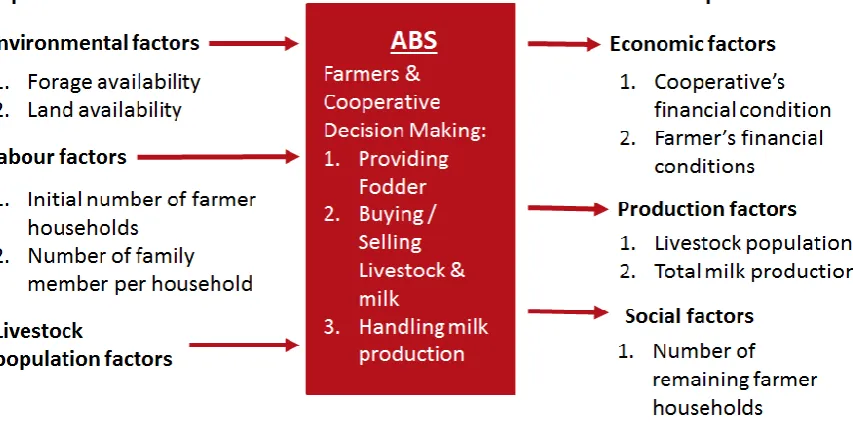
This model aims to replicate outputs such as milk production, cow population and number of
farmer household trends in Pangalengan. We selected these parameters because they are
considered to be important by policymakers as such they collect these statistics annually. To
produce these outputs, the model uses several inputs such as the initial number of farmer
households, number of family labour, cattle ownership, and cow’s productivity. Using these
inputs, the ABS simulates how agents make decisions such as when to buy or sell their cows,
and how to determine milk buying price based on its quality. Figure 3 describes the inputs and
Figure 3 Input and output parameters in the simulation
Following the suggestion from Macal and North (2010), we then specified the agents, their
attributes, relationships and behaviours based on this body of knowledge. We used NetLogo
(Wilensky, 1999) programming platform to implement the conceptual model. After the
simulation implementation, we carried out verification and sensitivity analysis to eliminate
errors in our ABS. We presented and discussed our ABS in front of with an expert panel in
Indonesia to face validate it. This panel comprised of university researchers and policymakers
from the Animal Husbandry Department, and an experienced farmer. The face-validation
aimed at ensuring that our ABS has some correspondence with the reality and that its behaviour
can be accepted rationally (Schmid, 2005) by the expert. As suggested by
Sonderegger-Wakolbinger and Stummer (2015), in this face-validation process, the experts could
recommend revisions on the assumptions, the agent’s behaviour and the parameter values used
in our ABS. We then used the experts’ suggestions to adjust and to improve our ABS described
below.
3. Model description
The ABS of dairy supply chain in Pangalengan involves three types of agents namely, a number
of separate farmer households, a cooperative and patches. The farmer households’ role is to
produce milk and supply the cooperative. The cooperative sets the milk price based on the milk
quality and then sells the milk to the milk processing industry. The farmers interact with the
patches whose main function is to provide forage for their cows. The conditions in the case
of the agents in the system may vary. The simulation operates on daily time step, although
some processes occur on a monthly and annual schedule.
3.1.The patch agent
One patch represents one kilometre square area (in total there are 306 patches in the model). In
the simulation, there are three types of patch (i.e., used patch, unused patch and forage patch).
Used patches represent the land area that has been occupied by building, houses, roads, etc.
Unused patches represent empty land areas that are not suitable to grow forage but can be used
to build new cattle pens. Forage patches represent land areas that are currently overgrown with
forage.
Every day the forage patches produce forage. The amount of forage production on these patches
(kg per km2 per day) is defined as a function of the amount forage grow and forage taken, as
described in equation 1.
𝑑𝐹
𝑑𝑡 = 𝑀𝑖𝑛((𝐹𝑚𝑎𝑥 − 𝐹𝑡− 𝐹𝑐𝑡), (𝐹𝑡− 𝐹𝑐𝑡) ∗ (1 + 𝐺))
(1)
𝐹𝑚𝑎𝑥 represents the maximum amount of forage (kg) in one kilometre square area. There are
various forage grass species in the case study area, and observation about the actual
composition is not available. However, (Bahar, 2014) estimated the forage productivity of
various grass composition that can grow in one kilometre square area in Indonesia is between
270 and 734 (tonnes per km2). Hence, in each run, the maximum amount of forage that can
grow on a patch is randomized within this range. 𝐹𝑡 is the initial forage level and 𝐹𝑐𝑡 is the
amount of forage taken by the farmers on the given day. G represents the forage growth rate,
which average value is 1.1% (per day) (Bahar, 2014) and it is taken as a constant. Other factors
such as precipitation (Gross et al., 2006), are neglected in the current model version.
3.2.The farmer household agent
A farmer household agent consists of several family members who work together to rear cattle.
Each farmer household has several attributes. We modelled some of the farmer’s attributes as
variables (e.g., money, number of cattle, pen area and type of transportation mode). Other
farmer attributes are modelled as lists (e.g., family members’ age, cattle gender, cattle age, the
percentage of fodder fulfilment, services per conception and maximum milk production). Each
and the maximum milk that can be produced by each cow respectively. The elements in these
lists only have a non-zero value for the cows.
We assume that the farmers accumulate their assets over time, this is in line with the previous
studies such as (Gross et al., 2006, Boone et al., 2011). Farmers’ assets in this simulation consist
of money and cattle. Farmers’ income comes from milk and cattle selling, and they use their
money to pay monthly living expenses. Based on the discussions with the experts, very few
farmers have sources of income other than producing and selling milk. This is because rearing
dairy cattle is very time-consuming. Therefore, our model assumes that the farmers do not
produce crops or have off-farm jobs. To increase their assets, we assume that farmers have
strategies to collect forage, sell milk, sell cattle, buy cattle and expand pen area, this assumption
is also in line with previous studies such as Gross et al. (2006) and Boone et al. (2011).
3.2.1.Forage collection procedure
Every day farmers collect forage to feed their cattle. They scan forage patches around their
house. The maximum distance they can travel is constrained by the number of working hours
and the speed of the transportation mode at their disposal. Each farmer household typically has
8 hours per day to collect forage, after and before they send milk to the cooperative (the
cooperative collect milk from farmers at 7 am and 3 pm). In the case study area, the farmers
collect forage by walking, motorcycle or truck. In line with Martin et al. (2016), farmers are
assumed to prioritise the location with the highest forage level when choosing the location to
collect forage. If there is more than one location with the highest forage level, then agents
prioritise forage collection from the closest location to their house.
Having decided the location to collect forage, the agents move to the designated patch. Their
travel time is taken away from their remaining working hours. The amount of forage they can
collect from the given patch is constrained by the patch’s forage level, the number of family
labour, their remaining working hours and their transport capacity. Actual measurements
regarding these variables are not available. Hence we asked the expert to suggest reasonable
approximations based on their experience. The expert suggested that each family labour can
harvest 40 kg of forage per hour. Further, the expert approximated that they can carry 40 kg of
forage per person per trip if they transport the forage on their back or using a cart, 60 kg of
forage per trip if they use motorcycle and 600 kg of forage per trip if they use a truck.
Farmer agents use the forage to feed their cattle. One cattle require 40 kg of fodder per day
which is consists of forage and additional fodder. The expert suggested that to stay healthy, a
cattle requires 30 kg of forage a day. For the cows, the forage fulfilment also affects the quantity
of the milk they produce. However, the expert suggested that the farmers usually substitute
forage with additional fodder whenever they cannot collect sufficient amount of forage for their
cattle. This is also in common with a previous study that assumed the level of additional fodder
used is affected by the forage availability Gross et al. (2006).
3.2.3.Milk production procedure
Farmers’ cows which have been pregnant can produce milk. The first pregnancy usually occurs after the cow’s age reaches two years old. The quantity of milk produced is determined by
several factors (i.e., age, genetics and forage), which is described in equation 2.
𝑄𝑚𝑖 = {𝑀𝑎𝑥𝑃𝑟𝑜𝑑𝑖∗ 𝑁𝑢𝑚𝑃𝑟𝑒𝑔𝑖∗ 𝐹𝑜𝑟𝑎𝑔𝑒̅̅̅̅̅̅̅̅̅̅𝑖 , 𝑃𝑟𝑒𝑔𝑃𝑒𝑟𝑖𝑜𝑑 < 7 𝑚𝑜𝑛𝑡ℎ 0 , 𝑃𝑟𝑒𝑔𝑃𝑒𝑟𝑖𝑜𝑑 > 7 𝑚𝑜𝑛𝑡ℎ
(2)
𝑄𝑚𝑖 denotes the quantity of milk produced by cow i in a day. The 𝑃𝑟𝑒𝑔𝑃𝑒𝑟𝑖𝑜𝑑 variable
represents how long the given cow has been pregnant. The farmers usually stop milking a cow
which has been pregnant for 7 months and restart the milking process after it gives birth. Hence
the milk production during this period is zero. 𝑀𝑎𝑥𝑃𝑟𝑜𝑑𝑖 denotes the maximum milk
production which represents the genetic attribute of the given cow. 𝑁𝑢𝑚𝑃𝑟𝑒𝑔𝑖 denotes how
many times the given cow has ever been pregnant and it represents the age factor. The expert
suggest that a cow achieves its maximum milk production after the second pregnancy
(𝑁𝑢𝑚𝑃𝑟𝑒𝑔𝑖(2)= 100%), the milk production then decreases in the subsequent pregnancies. Actual measurements to establish this function are not available. However, the expert
suggested that it is reasonable to assume that the milk production is decreasing linearly. We
also assume that the milk production is proportional to the 𝐹𝑜𝑟𝑎𝑔𝑒̅̅̅̅̅̅̅̅̅̅𝑖 which represents the
average forage fulfilment (between 0 and 1) of cow i. The average forage fulfilment of 1 means
that the given cattle always obtain sufficient forage throughout its lifetime.
In addition to the quantity, we also consider the milk quality in our simulation. This variable
determines the milk price per litre received from the cooperative. The expert suggested that the
milk quality is determined by the average proportion of forage from the total fodder.
Accordingly, the highest milk quality is achieved when the average proportion of forage is
quality decreases and this leads them receiving a lower milk price. We model the relationship
between forage proportion and milk quality as a linear function in which the milk quality value
is 100% when the forage proportion is 75% or higher.
3.2.4.Cattle selling and buying procedures
Decisions regarding how many cattle should be retained are the most important decision made
by the farmer agents because it would affect the amount of forage required, cattle weight,
mortality and the amount of additional fodder used (Gross et al., 2006). In this ABS three
separate procedures rule how the farmers buy or sell their cattle. In the first procedure, the
decision to sell or buy cattle is triggered by the forage availability (Gross et al., 2006, Lie and
Rich, 2016, Lie et al., 2017). In the second procedure, this decision is triggered by the cattle’s
age (Rasch et al., 2016, Rasch et al., 2017). Finally, the last procedure is triggered by farmers’
financial condition (Boone et al., 2011).
In line with the previous study (Gross et al., 2006, Lie and Rich, 2016, Lie et al., 2017), in the
first procedure, we assume that the forage availability is a trigger for the farmers to sell or buy
cattle. When the forage is less available (e.g., during a drought), they sell some of their cattle
and, conversely, buy new cattle (cows in particular) when the forage becomes more available.
We assume that the farmers sell or buy their cattle to an external agent outside the system and
not to other farmers (Boone et al., 2011, Lie and Rich, 2016, Lie et al., 2017, Rasch et al., 2016,
Rasch et al., 2017).
Our ABS assumes that the farmers can make a short-term forecast of forage availability when
deciding whether to sell or buy cattle. They do this by calculating the average forage they
obtain each day. If the average forage collected is less than the amount of forage required to
feed all of their cattle the farmers will start to sell their cattle. According to the experts, since
the bulls do not generate routine income, the farmers will prioritise to sell them first. Only
when they do not have any more bulls will they start to consider selling their cows. When
selling the cows, farmer agents compare the potential income they can obtain by feeding less
forage but retaining all of their cows (equation 3), and the potential income they can obtain by
selling some of their cows in order to feed the remaining cows with sufficient forage (equation
𝑖𝑛𝑐𝑜𝑚𝑒𝑟𝑒𝑡𝑎𝑖𝑛 = #𝐶𝑜𝑤 ((𝑄𝑚̅̅̅̅̅ ∗ 𝑀𝑃̅̅̅̅̅ ∗ 𝐹𝑐 ̅̅̅
#𝑐𝑜𝑤 ⁄
30 ) − ((10 + 30 −
𝐹𝑐 ̅̅̅
#𝐶𝑜𝑤) ∗ 𝐴𝑓𝑃)) (3)
𝑖𝑛𝑐𝑜𝑚𝑒𝑠𝑒𝑙𝑙 =𝐹𝑐̅̅̅
30((𝑄𝑚̅̅̅̅̅ ∗ 𝑀𝑃̅̅̅̅̅) − (10 ∗ 𝐴𝑓𝑃))
(4)
In equation 3 and equation 4 equations #cow denotes the number of cows currently owned by
a farmer. 𝐹𝑐̅̅̅ represents the average forage obtained by the farmer and 𝐹𝑐̅̅̅⁄30 represents the
maximum number of cow the farmer can retain for the given forage availability. 𝑄𝑚̅̅̅̅̅ , 𝑀𝑃̅̅̅̅̅ and
𝐴𝑓𝑃 represent the average milk production per cow, the average milk price per litre and the
additional fodder price respectively. In equation 3, the farmer has more cows to produce milk
but suffers a production penalty owing to the lack of forage and must pay more for extra
additional fodder. In equation 4, the farmer has fewer cows but each cow can produce more
milk and the agent does not need to buy extra additional fodder. If 𝑖𝑛𝑐𝑜𝑚𝑒𝑠𝑒𝑙𝑙 > 𝑖𝑛𝑐𝑜𝑚𝑒𝑟𝑒𝑡𝑎𝑖𝑛
then the farmer will decide to sell the cows and vice versa.
Our ABS assumes that when selling cattle the farmers will prioritise to sale the oldest cattle
first, this is in line with the previous modelling studies (e.g., Boone et al. (2011)). The farmers
use this priority because an older animal usually has more live weight and more valuable
(Quang et al., 2014). For the cows, in addition to having more live weight, the milk productivity
of an older cow has decreased.
On the contrary, if the farmers can collect more forage than is needed, then they start to consider
to buy more cows. The number of new cows a farmer is willing to buy is proportional to the
additional cows that can be fed using the excess forage (see equation 5).
𝐴𝑑𝑑_𝐶𝑜𝑤 = {𝑅𝑜𝑢𝑛𝑑𝑒𝑑𝑑𝑜𝑤𝑛 (𝐹𝑐
̅̅̅ 30
⁄ − #𝑐𝑜𝑤) , if (𝐹𝑐̅̅̅⁄30− #𝑐𝑜𝑤) > 0
0 , if (𝐹𝑐̅̅̅⁄30− #𝑐𝑜𝑤) ≤ 0
(5)
The constraints in the buying decisions are the pen capacity and the farmer’s money. If the
farmer owns sufficient pen capacity to contain all of his/her cows (including the new cows),
then the farmer only needs to have enough money to buy the cows. However, if the farmer does
not have sufficient pen capacity, then he/she must have enough money to buy the cows and to
land availability on the patch where he/she is living. The fertility and productivity of newly
bought cows are assumed to be random.
In the second procedure, a farmer decides to sell his/her cattle by considering the cattle’s age.
The bulls are commonly sold at two years old. According to experts, farmers believe that the
bulls have reached their optimum live weight at this age. Meanwhile, the cows are commonly
culled when they reach the age of 10 years. It is believed that at ten years old a cow’s milk
productivity has become too low. In future research, we will collect data regarding the actual
age at which the bulls are sold, and the cows are culled.
In the third procedure, a farmer decides to sell his/her cattle by considering his/her financial
condition. Each month, the farmer agent forecasts the amount of money it will have at the end
of the month by taking into account the income it earned in the previous month and the living
expenses it must pay. The living expense value is calculated by multiplying the number of the
farmer’s family members and the standard cost of living in the area. If the forecasted amount
of money is less than the living expense value, then the farmer agent starts to consider selling
its cattle. As in the first procedure, the farmers are assumed to sell the bulls first. In this
procedure, we also assume that the farmers select the cattle to sell based on the age. The selling
process is repeated until the farmer’s money deficit is covered.
In all of those three procedures, the price received by the farmer agent when selling their cattle
is assumed to be proportional to the age of cattle being sold (see equation 6 and 7). In these
equations, Bull price and Cow price denote the money that will be received by the farmer agent.
𝐴𝑔𝑒𝑖 denotes the age of the animal being sold in moths. Max Bull Age and Max Cow Age
represent how long an animal is usually retained by farmers (i.e., 24 months for a bull and 120
months for a cow). Finally, Max Bull Price and Max Cow Price represent the price of bull and
cow that is sold at optimum live weight i.e., 16 and 13 million rupiahs (Indonesian currency)
respectively.
Bull_price = 𝐴𝑔𝑒𝑖
𝑀𝑎𝑥_𝐵𝑢𝑙𝑙_𝐴𝑔𝑒∗ 𝑀𝑎𝑥_𝐵𝑢𝑙𝑙_𝑃𝑟𝑖𝑐𝑒
(6)
Cow_price = 𝐴𝑔𝑒𝑖
𝑀𝑎𝑥_𝐶𝑜𝑤_𝐴𝑔𝑒∗ 𝑀𝑎𝑥_𝐶𝑜𝑤_𝑃𝑟𝑖𝑐𝑒
(7)
When a farmer decides to buy a new cow, the price that must be paid is assumed to be constant,
3.2.5.Cow reproduction
In the previous studies the cow reproduction is commonly modelled with a fixed schedule (e.g.,
annually) or growth rate (e.g., increase the population by 10% every year) (e.g., Gross et al.
(2006), Rasch et al. (2016), Martin et al. (2016), Rasch et al. (2017)). Our ABS considers cow
fertility factor that is heterogeneous. In cow reproduction procedure, the farmers artificially
inseminate those cows who are two years old or older and not pregnant at the beginning of each
simulation month. The successfulness of the artificial insemination process depends on the
cow's fertility, which is represented by the services per conception variable. If the artificial
insemination fails, then this process would be repeated in the subsequent month.
If the artificial insemination process is successful, then the pregnancy process lasts for nine
months. The cow then gives birth to either a male or female calf each with 50% probability. If
the cow gives birth to a female calf, then the newborn calf inherits the milk productivity and
fertility of its parent.
3.2.6.Farmer households retirement and succession
There are two main factors affecting farmer retirement and succession namely, age and
financial condition. At the end of each simulation year, all farmer household members who are
older than 72 years old (the productive age in the case study area) are removed from the farmer
household family member list and the number of family labour decreases. A farmer household
agent can also acquire a new family member with a probability of 1.2% (the average population
growth in Indonesia). A farmer household agent is deleted from the simulation if it does not
have any family member left or if it runs out of money and cattle.
Probabilistically, a new farmer household can be generated in the simulation. Its attributes are
defined based on the input parameters, as in the initiation procedure of farmer household
agents. However, as we mentioned earlier, owing to population growth, the farmland that was
once located in the rural area is currently surrounded by residential areas. The existence of a
farmer household who continue dairy farming is tolerated by the non-farmers because they are
native to the area while the non-farmers are mainly newcomers. The cooperative’s database
also shows that all of its members are farmer families from generation to generation. However,
conflict with non-farmers could spark easily if a newcomer tries to start dairy farming. This
conflict is usually triggered by pollution caused by manure production and potential water
be sold and converted into residential area settlement or another business. Our simulation aims
to replicate the reality in the case study area so the probability of a new farmer household agent
entering the system is set to be equal to zero.
3.3.The cooperative agent
The cooperative agent collects and grades milk from all farmer household agents. We assume
that the cooperative determine the milk buying price as a linear function of milk quality,
ranging from 3350 to 5200 (IDR per litre). Based on the discussion with the experts, the
cooperative sell the milk to the milk processing industry at a fixed price. The actual buying
price from the milk processing industry is unknown, but the experts estimated that it is
approximately 5500 (IDR per litre). The experts agreed that the cooperative’s daily operational
costs could be assumed to be fixed regardless of the total volume of milk they handle. Hence,
it is more profitable if they can operate at full capacity.
4. Simulation experiments
This section discusses simulation experiments aim to analyse the output of the model. To
validate the ABS the real cattle population, cow population, milk production and the number
of farmer households data obtained from the farmer cooperative (KPBS, 2016) are used. The
number of agents involved in these experiments was 5700 farmer households; this is in line
with the number of farmers in the case study area in January 2010.
The ABS was run for five simulation years (from January 2010 to December 2014) and
replicated 30 times. The simulation data in Figures 4 to 7 represent the average of 30 simulation
Figure 4 the number of surviving farmer household
Figure 5 the cow population
0 500 1000 1500 2000 2500 3000 3500 4000 4500
Jan-11 Jan-12 Jan-13 Jan-14 Jan-15
# Fa
rm
er
H
o
u
se
h
o
ld
Real Data
Simulation Data
0 5000 10000 15000 20000 25000
Jan-11 Jan-12 Jan-13 Jan-14 Jan-15
Cow
(Head
s)
Real Data
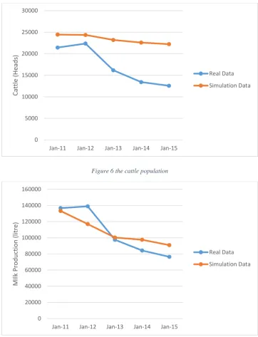
[image:14.595.117.479.336.563.2]Figure 6 the cattle population
Figure 7 the daily milk production
These experiments show that the number of farmer household, cow population, cattle
population and the daily milk production tend to decrease overtime. Figures 4 to 7 show that
these patterns correspond to real data obtained from the farmer’s cooperative. Thus the ABS
presented in this working paper has sufficient validity.
5. Conclusion
This working paper has described a case study of dairy supply chain in West Java Indonesia.
We have discussed the process to model this dairy supply chain using ABS. Our ABS has some
uniqueness compared to previous ABS applications because it features dyadic interactions 0
5000 10000 15000 20000 25000 30000
Jan-11 Jan-12 Jan-13 Jan-14 Jan-15
Catt
le
(Head
s)
Real Data
Simulation Data
0 20000 40000 60000 80000 100000 120000 140000 160000
Jan-11 Jan-12 Jan-13 Jan-14 Jan-15
MIlk
P
ro
d
u
ctio
n
(litre)
Real Data
between the farmers and the cooperative. Moreover, it considers the heterogeneity of cow’s
fertility and milk productivity. The simulation experiments show that the output of our ABS
has high correspondence with the real-world data. In the future study, we plan to collect
primary data to calibrate this ABS empirically.
6. References
BAHAR, S. 2014. Produktivitas hijauan pakan untuk produksi sapi potong di Sulawesi Selatan.
JITV, 19.
BOONE, R., GALVIN, K., BURNSILVER, S., THORNTON, P., OJIMA, D. & JAWSON, J. 2011. Using coupled simulation models to link pastoral decision making and ecosystem
services. Ecology and Society, 16.
DAUD, A., PUTRO, U. & BASRI, M. 2015. Risks in milk supply chain; a preliminary analysis
on smallholder dairy production. Livestock Research for Rural Development, 27, 137.
GILBERT, N. 2004. Agent-based social simulation: dealing with complexity. The Complex
Systems Network of Excellence, 9, 1-14.
GLOCK, C. H. 2012. Coordination of a production network with a single buyer and multiple
vendors. International Journal of Production Economics, 135, 771-780.
GLOVER, J. L., CHAMPION, D., DANIELS, K. J. & DAINTY, A. J. D. 2014. An Institutional
Theory perspective on sustainable practices across the dairy supply chain. International
Journal of Production Economics, 152, 102-111.
GROSS, J. E., MCALLISTER, R. R. J., ABEL, N., SMITH, D. M. S. & MARU, Y. 2006. Australian rangelands as complex adaptive systems: a conceptual model and
preliminary results. Environmental Modelling & Software, 21, 1264-1272.
HAPPE, K., HUTCHINGS, N. J., DALGAARD, T. & KELLERMAN, K. 2011. Modelling the interactions between regional farming structure, nitrogen losses and environmental
regulation. Agricultural Systems, 104, 281-291.
HAPPE, K., SCHNICKE, H., SAHRBACHER, C. & KELLERMANN, K. 2009. Will They Stay or Will They Go? Simulating the Dynamics of Single-Holder Farms in a Dualistic
Farm Structure in Slovakia. Canadian Journal of Agricultural Economics/Revue
canadienne d'agroeconomie, 57, 497-511.
KPBS 2016. Data Populasi dan Penghasilan Anggota KPBS. Unpublished Dataset.
LIE, H. & RICH, K. M. 2016. Modeling Dynamic Processes in Smallholder Dairy Value
Chains in Nicaragua: A System Dynamics Approach. International Journal on Food
System Dynamics, 7, 328-340.
LIE, H., RICH, K. M. & BURKART, S. 2017. Participatory system dynamics modelling for
dairy value chain development in Nicaragua. Development in Practice, 27, 785-800.
MACAL, C. & NORTH, M. 2010. Tutorial on agent-based modelling and simulation. Journal
of Simulation, 4, 151-162.
MANISH, S. & SANJAY, J. 2013. Agri‐fresh produce supply chain management: a state‐of‐
the‐art literature review. International Journal of Operations & Production
Management, 33, 114-158.
MAROHN, C., SCHREINEMACHERS, P., QUANG, D. V., BERGER, T.,
SIRIPALANGKANONT, P., NGUYEN, T. T. & CADISCH, G. 2013. A software coupling approach to assess low-cost soil conservation strategies for highland
MARTIN, R., LINSTÄDTER, A., FRANK, K. & MÜLLER, B. 2016. Livelihood security in
face of drought – Assessing the vulnerability of pastoral households. Environmental
Modelling & Software, 75, 414-423.
QUANG, D. V., SCHREINEMACHERS, P. & BERGER, T. 2014. Ex-ante assessment of soil conservation methods in the uplands of Vietnam: An agent-based modeling approach.
Agricultural Systems, 123, 108-119.
RASCH, S., HECKELEI, T., OOMEN, R. & NAUMANN, C. 2016. Cooperation and collapse in a communal livestock production SES model – A case from South Africa.
Environmental Modelling & Software, 75, 402-413.
RASCH, S., HECKELEI, T., STORM, H., OOMEN, R. & NAUMANN, C. 2017. Multi-scale
resilience of a communal rangeland system in South Africa. Ecological Economics,
131, 129-138.
SCHMID, A. 2005. What is the Truth of Simulation? Journal of Artificial Societies and Social
Simulation, 8.
SONDEREGGER-WAKOLBINGER, L. M. & STUMMER, C. 2015. An agent-based
simulation of customer multi-channel choice behavior. Central European Journal of
Operations Research, 23, 459.
UTOMO, D. S., ONGGO, B. S. & ELDRIDGE, S. 2018. Applications of agent-based
modelling and simulation in the agri-food supply chains. European Journal of
Operational Research, 269, 794-805.
WILENSKY, U. 1999. NetLogo: Center for Connected Learning Comp.-Based Modeling.