warwick.ac.uk/lib-publications
Manuscript version: Working paper (or pre-print)
The version presented here is a Working Paper (or ‘pre-print’) that may be later published elsewhere.
Persistent WRAP URL:
http://wrap.warwick.ac.uk/130832
How to cite:
Please refer to the repository item page, detailed above, for the most recent bibliographic citation information. If a published version is known of, the repository item page linked to above, will contain details on accessing it.
Copyright and reuse:
The Warwick Research Archive Portal (WRAP) makes this work by researchers of the University of Warwick available open access under the following conditions.
Copyright © and all moral rights to the version of the paper presented here belong to the individual author(s) and/or other copyright owners. To the extent reasonable and practicable the material made available in WRAP has been checked for eligibility before being made available.
Copies of full items can be used for personal research or study, educational, or not-for-profit purposes without prior permission or charge. Provided that the authors, title and full
bibliographic details are credited, a hyperlink and/or URL is given for the original metadata page and the content is not changed in any way.
Publisher’s statement:
Please refer to the repository item page, publisher’s statement section, for further information.
Warwick Economics Research Papers
ISSN 2059-4283 (online)
ISSN 0083-7350 (print)
High Dimensional Latent Panel Quantile Regression with an
Application to Asset Pricing
Alexandre Belloni, Mingli Chen, Oscar Hernan Madrid Padilla, and Zixuan (Kevin) Wang
High Dimensional Latent Panel Quantile Regression
with an Application to Asset Pricing
∗Alexandre Belloni1, Mingli Chen2, Oscar Hernan Madrid Padilla3, and Zixuan (Kevin) Wang4
1Fuqua Business School, Duke University
2Department of Economics, University of Warwick 3Department of Statistics, University of California, Los Angeles
4Harvard University
December 4, 2019
Abstract
We propose a generalization of the linear panel quantile regression model to accommodate
bothsparseanddense parts: sparse means while the number of covariates available is large, potentially only a much smaller number of them have a nonzero impact on each conditional
quantile of the response variable; while the dense part is represented by a low-rank matrix that can be approximated by latent factors and their loadings. Such a structure poses problems for traditional sparse estimators, such as the`1-penalised Quantile Regression, and for traditional
latent factor estimator, such as PCA. We propose a new estimation procedure, based on the ADMM algorithm, that consists of combining the quantile loss function with`1 andnuclear
norm regularization. We show, under general conditions, that our estimator can consistently estimate both the nonzero coefficients of the covariates and the latent low-rank matrix.
Our proposed model has a “Characteristics + Latent Factors” Asset Pricing Model
interpre-tation: we apply our model and estimator with a large-dimensional panel of financial data and find that (i) characteristics have sparser predictive power once latent factors were controlled (ii)
the factors and coefficients at upper and lower quantiles are different from the median.
Keywords: High-dimensional quantile regression; factor model; nuclear norm regulariza-tion; panel data; asset pricing; characteristic-based model
∗
1
Introduction
A central question in asset pricing is to explain the returns of stocks. According to the Arbitrage Pricing Theory, when the asset returns are generated by a linear factor model, there exists a stochastic discount factor linear in the factors that prices the returns (Ross(1976),Cochrane (2009)). However, from an empirical
perspective, testing the theory is difficult because the factors are not directly observed.
To overcome this challenge, one approach uses characteristic-sorted portfolio returns to mimic the un-known factors. This approach for understanding expected returns can be captured by the following panel
data model (Cochrane(2011)):
E(Yi,t|Xi,t−1) =Xi,t0 −1θ. (1)
The drawback of this approach is that it requires a list of pre-specified characteristics which are chosen based on empirical experience and thus somewhat arbitrarily (Fama and French(1993)). In addition, the
lit-erature has documented a zoo of new characteristics, and the proliferation of characteristics in this “variable zoo” leads to the following questions: “which characteristics really provide independent information about average returns, and which are subsumed by others?” (Cochrane(2011)). Another approach uses
statisti-cal factor analysis, e.g. Principal Component Analysis (PCA), to extract latent factors from asset returns (Chamberlain and Rothschild(1983),Connor and Korajczyk(1988)):
E(Yi,t) =λ0igt. (2)
However, one main critique with this approach is that the latent factors estimated via PCA are purely statis-tical factors, thus lacks economic insightCampbell(2017).
We extend both modeling approaches and propose a “Characteristics + Latent Factors” framework. By incorporating the “Characteristics” documented, we improve the economic interpretability and explanatory power of the model. The characteristics can have asparsestructure, meaning although a large set of variables
is available, only a much smaller subset of them might have predictive power. We also incorporate “Latent Factors”, one benefit of having this part is that it might help alleviate the “omitted variable bias” problem (Giglio and Xiu (2018)). As in the literature typically these latent factors are estimated via PCA, which
means all possible latent explanatory variables (those are not included in the model) might be important for prediction although their individual contribution might be small, we term this as thedensepart.1
Hence, our framework allows for “Sparse + Dense” modeling with the time series and cross-section of
asset returns. In addition, we focus on understanding the quantiles (hence the entire distribution) of returns rather than just the mean, in line with recent interest in quantile factor models (e.g. Ando and Bai(2019),
Chen et al.(2018),Ma et al.(2019),Feng(2019), andSagner(2019)). Specifically, we study the following high dimensional latent panel quantile regression model withY ∈Rn×T andX∈Rn×T×psatisfying
FY−1
i,t|Xi,t;θ(τ),λi(τ),gt(τ)(τ) = X
0
i,tθ(τ) +λi(τ) 0
gt(τ), i = 1. . . , n, t = 1, . . . , T, (3)
1
whereidenotes subjects (or assets in our asset pricing setting),tdenotes time,θ(τ) ∈ Rp is the vector of
coefficients,λi(τ), gt(τ) ∈Rrτ withrτ min{n, T}(denoteΠi,t(τ) =λi(τ)0gt(τ), thenΠ(τ) ∈Rn×T is a low-rank matrix with unknown rankrτ),τ ∈[0,1]is the quantile index, andFYi,t|Xi,t;θ(τ),λi(τ),gt(τ)(or
FYi,t|Xi,t;θ(τ),Πi,t(τ)) is the cumulative distribution function ofYi,tconditioning onXi,t,θ(τ)andλi(τ), gt(τ) (orΠi,t(τ)). Our framework also allows for the possibility of lagged dependent data. Thus, we model the
quantile function at level τ as a linear combination of the predictors plus a low-rank matrix (or a factor structure). Here, we allow for the number of covariatesp, and the time horizonT, to grow to infinity asn
grows. Throughout the paper we mainly focus on the case wherepis large, possibly much larger thannT,
but for the true modelθ(τ)is sparse and has onlysτ pnon-zero components.
Our framework is flexible enough that allows us to jointly answer the following three questions in asset pricing: (i) Which characteristics are important to explain the time series and cross-section of stock
returns, after controlling for the factors? (ii) How much would the latent factors explain stock returns after controlling for firm characteristics? (iii) Does the relationship of stock returns and firm characteristics change across quantiles? The first question is related to the recent literature on variable selection in asset
pricing using machine learning (Kozak et al. (2019);Feng et al. (2019); Han et al. (2018)). The second question is related to an classical literature starting from 1980s on statistical factor models of stock returns
(Chamberlain and Rothschild(1983);Connor and Korajczyk(1988) and recentlyLettau and Pelger(2018)). The third question extends the literature in late 1990s on stock return and firm characteristics (Daniel and Titman(1997,1998)) and further asks whether the relationship is heterogenous across quantiles.
There are several key features of considering prediction problem at the panel quantile model in this setting. First, stock returns are known to be asymmetric and exhibits heavy tail, thus modeling different quantiles of return provides extra information in addition to models of first and second moments. Second,
quantile regression provides a richer characterization of the data, allowing heterogeneous relationship be-tween stock returns and firm characteristics across the entire return distribution. Third, the latent factors
might also be different at different quantiles of stock returns. Finally, quantile regression is more robust to the presence of outliers relative to other widely used mean-based approaches. Using a robust method is crucial when estimating low-rank structures (see e.g.She and Chen(2017)). As our framework is based on
modeling the quantiles of the response variable, we do not put assumptions directly on the moments of the dependent variable.
Our main goal is to consistently estimate both the sparse part and the low-rank matrix. Recovery of a
low-rank matrix, when there are additional high dimensional covariates, in a nonlinear model can be very challenging. The rank constraint will result in the optimization problem NP-hard. In addition, estimation in high dimensional regression is known to be a challenging task, which in our frameworks becomes even more
difficult due to the additional latent structure. We address the former challenge via nuclear norm regulariza-tion which is similar toCand`es and Recht(2009) in the matrix completion setting. Without covariates, the
recovery of the underlying low-rank structure. We address the latter challenge by imposing`1regularization
on the vector of coefficients of the control variables, similarly toBelloni and Chernozhukov(2011) which mainly focused on the cross-sectional data setting. Note that with regards to sparsity, we must be cautious,
specially when considering predictive models (She and Chen(2017)). Furthermore, we explore the perfor-mance of our procedure under settings where the vector of coefficients can be dense (due to the low-rank
matrix).
We also propose a novel Alternating Direction Method of Multipliers (ADMM) algorithm (Boyd et al.
(2011)) that allows us to estimate, at different quantile levels, both the vector of coefficients and the low-rank matrix. Our proposed algorithm can easily be adjusted to other nonlinear models with a low-rank matrix
(with or without covariates).
We view our work as complementary to the low dimensional quantile regression with interactive fixed effects framework as of the recent work ofFeng(2019), and the mean estimation setting inMoon and
Weid-ner(2018). However, unlikeMoon and Weidner(2018) andFeng(2019), we allow the number of covariates
p to be large, perhapsp nT. This comes with different significant challenges. On the computational
side, it requires us to develop novel estimation algorithms, which turns out can also be used for the contexts inMoon and Weidner(2018) andFeng(2019). On the theoretical side, allowingp nT requires a sys-tematically different analysis as compared toFeng(2019), as it is known that ordinary quantile regression
is inconsistent in high dimensional settings (pnT), seeBelloni and Chernozhukov(2011).
Related Literature. Our work contributes to the recent growing literature on panel quantile model. Abre-vaya and Dahl(2008),Graham et al.(2018),Arellano and Bonhomme(2017), considered the fixedT
asymp-totic case.Kato et al.(2012) formally derived the asymptotic properties of the fixed effect quantile regression estimator under largeT asymptotics, andGalvao and Kato(2016) further proposed fixed effects smoothed quantile regression estimator. Galvao(2011) works on dynamic panel. Koenker(2004) proposed a
penal-ized estimation method where the individual effects are treated as pure location shift parameters common to all quantiles, for other related literature seeLamarche (2010),Galvao and Montes-Rojas(2010). We refer
to Chapter 19 ofKoenker et al.(2017) for a review.
Our work also contributes to the literature on nuclear norm penalisation, which has been widely studied in the machine learning and statistical learning literature,Fazel(2002),Recht et al.(2010);Koltchinskii et al.
(2011);Rohde and Tsybakov(2011),Negahban and Wainwright(2011),Brahma et al.(2017). Recently, in the econometrics literatureAthey et al.(2018) proposes a framework of matrix completion for estimating causal effects, Bai and Ng (2017) for estimating approximate factor model, Chernozhukov et al.(2018)
considered the heterogeneous coefficients version of the linear panel data interactive fixed model where the main coefficients has a latent low-rank structure, Bai and Feng(2019) for robust principal component
Finally, our results contribute to a growing literature on high dimensional quantile regression.Wang et al.
(2012) considered quantile regression with concave penalties for ultra-high dimensional data;Zheng et al.
(2015) proposed an adaptively weighted`1-penalty for globally concerned quantile regression. Screening
procedures based on moment conditions motivated by the quantile models have been proposed and analyzed inHe et al.(2013) andWu and Yin(2015) in the high-dimensional regression setting. We refer toKoenker
et al.(2017) for a review.
To sum-up, our paper makes the following contributions. First, we propose a new class models that consist of bothhigh dimensional regressorsandlatent factorstructures. We provide a scalable estimation procedure, and show that the resulting estimator is consistent under suitable regularity conditions. Second,
the high dimensional and non-smooth objective function require innovative strategies to derive all the above-mentioned results. This leads to the use in our proofs of some novel techniques from high dimensional
statistics/econometrics, spectral theory, empirical process, etc. Third, the proposed estimators inherit from quantile regression certain robustness properties to the presence of outliers and heavy-tailed distributions in the idiosyncratic component of a factor model. Finally, we apply our proposed model and estimator to a
large-dimensional panel of financial data in the US stock market and find that different return quantiles have different selected firm characteristics and that the number of latent factors can be also be different.
Outline. The rest of the paper is organized as follows. Section2introduces the high dimensional latent quantile regression model, and provides an overview of the main theoretical results. Section3presents the estimator and our proposed ADMM algorithm. Section4discusses the statistical properties of the proposed
estimator. Section5provides simulation results. Section 6consists of the empirical results of our model applied to a real data set. The proofs of the main results are in the Appendix.
Notation. For m ∈ N, we write [m] = {1, . . . , m}. For a vector v ∈ Rp we define its `
0 norm as
kvk0 =Pp
j=11{vj 6= 0}, where1{·}takes value1if the statement inside{}is true, and zero otherwise;
its`1 norm askvk1 = Ppj=1|vj|. We denotekvk1,n,T =Ppjσjˆ |vj|the`1-norm weighted byσjˆ ’s (details
can be found in eq (20)). The Euclidean norm is denoted byk · k, thuskvk = qPp
j=1vj2. IfA ∈ Rn×T
is a matrix, its Frobenius norm is denoted bykAkF =
q Pn
i=1
PT
t=1A2i,t, its spectral norm by kAk2 = supx:kxk=1
√
x0A0Ax, its infinity norm bykAk∞ = max{|Ai,j| : i∈[n], j ∈[T]}, its rank by rank(A),
and its nuclear norm bykAk∗ =trace(
√
A0A)whereA0is the transpose ofA. Thejth columnAis denoted
byA·,j. Furthermore, the multiplication of a tensorX ∈RI1×...×Im with a vectora∈ RIm is denoted by
Z := Xa ∈ RI1×...×Im−1, and, explicitly,Zi1,...i
m−1 =
PIm
j=1Xi1,...,im−1,jaj. We also use the notation a∨b= max{a, b},a∧b= min{a, b},(a)−= max{−a,0}. For a sequence of random variables{zj}∞j=1
we denote by σ(z1, z2, . . .) the sigma algebra generated by{zj}∞j=1. Finally, for sequences{an}∞n=1 and
{bn}∞n=1 we write an bn if there exists positive constantsc1 and c2 such that c1bn ≤ an ≤ c2bn for
2
The Estimator and Overview of Rate Results
2.1 Basic Setting
The setting of interest corresponds to a high dimension latent panel quantile regression model, whereY ∈
Rn×T, andX ∈Rn×T×p satisfying
FY−1
i,t|Xi,t;θ(τ),Πi,t(τ)(τ) = X
0
i,tθ(τ) + Πi,t(τ), i = 1. . . , n, t = 1, . . . , T, (4)
whereidenotes subjects,tdenotes time,θ(τ)∈Rpis the vector of coefficients,Π(τ)∈
Rn×T is a low-rank matrix with unknown rankrτ min{n, T},τ ∈[0,1]is the quantile index, andFYi,t|Xi,t;θ(τ),Πi,t(τ)is the cumulative distribution function ofYi,t conditioning onXi,t,θ(τ)andΠi,t(τ). Thus, we model the quantile
function at levelτ as a linear combination of the predictors plus a low-rank matrix. Here, we allow for the number of covariatesp, and the time horizonT, to grow to infinity asngrows. Throughout the paper the quantile indexτ ∈(0,1)is fixed. We mainly focus on the case wherepis large, possibly much larger thannT, but for the true modelθ(τ)is sparse and has onlysτ pnon-zero components. Mathematically, sτ :=kθ(τ)k0.
WhenΠi,t(τ) = λi(τ)0gt(τ), withλi(τ), gt(τ)∈Rrτ, this immediately leads to the following setting
FY−1
i,t|Xi,t;θ(τ),Πi,t(τ)(τ) = X
0
i,tθ(τ) +λi(τ)0gt(τ). (5)
where we model the quantile function at levelτ as a linear combination of the covariates (as predictors) plus a latent factor structure. This is directly related to the panel data models with interactive fixed effects literature in econometrics, e.g. linear panel data model (Bai(2009)), nonlinear panel data models (Chen
(2014);Chen et al.(2014)).
Note, for eq (5), additional identification restrictions are needed for estimatingλi(τ)andgt(τ)(seeBai and Ng(2013)). In addition, in nonlinear panel data models, this create additional difficulties in estimation,
as the latent factors and their loadings part are nonconvex.2
2.2 The Penalized Estimator, and its Convex Relaxation
In this subsection, we describe the high dimensional latent quantile estimator. With the sparsity and low-rank
constraints in mind, a natural formulation for the estimation of(θ(τ),Π(τ))is
minimize
˜
θ∈Rp, Π˜∈Rn×T
1
nT T
X
t=1
n
X
i=1
ρτ(Yi,t−Xi,t0 θ˜−Π˜i,t)
subject to rank( ˜Π)≤rτ,
kθ˜k0 =sτ,
(6)
2Different identification conditions might result in different estimation procedures forλandf, seeBai and Li(2012) andChen
whereρτ(t) = (τ −1{t ≤0})tis the quantile loss function as inKoenker(2005),sτ is a parameter that
directly controls the sparsity ofθ˜, andrτ controls the rank of the estimated latent matrix.
While the formulation in (6) seems appealing, as it enforces variable selection and low-rank matrix
estimation simultaneously, (6) is a non-convex problem due to the constraints posed by thek · k0andrank(·)
functions. We propose a convex relaxation of (6). Inspired by the seminal works ofTibshirani(1996) and
Cand`es and Recht(2009), we formulate the problem
min ˜
θ∈Rp, Π˜∈Rn×T
1
nT T
X
t=1
n
X
i=1
ρτ(Yi,t−Xi,t0 θ˜−Π˜i,t)
subject to kΠ˜k∗ ≤ν2,
p
X
j=1
wj|θj˜| ≤ν1,
(7)
whereν1 >0andν2 >0are tuning parameters, andw1, . . . , wp are user specified weights (more on this in
Section4).
In principle, one can use any convex solver software to solve (7), since this is a convex optimization problem. However, for large scale problems a more careful implementation might be needed. Section3.1
presents a scheme for solving (7) that is based on the ADMM algorithm ( (Boyd et al.,2011)).
2.3 Summary of results
We now summarize our main results. For the model defined in (4):
• Under (4), sτ min{n, T}, an assumption that implicitly requires rτ min{n, T}, and other
regularity conditions defined in Section4, we show that our estimator(ˆθ(τ),Π(ˆ τ))defined in Section
3 is consistent for(θ(τ),Π(τ)). Specifically, for the independent data case (acrossiandt), under suitable regularity conditions that can be found in Section4, we have
kθˆ(τ)−θ(τ)k = OP
√
sτmax{plogp,plogn,√rτ}
1
√
n+
1
√
T
. (8)
and
1
nTkΠ(ˆ τ)−Π(τ)k
2
F = OP
sτmax{logp,logn, rτ}
1
n+
1
T
, (9)
Importantly, the rates in (8) and (9), ignoring logarithmic factors, match those in previous works. However, our setting allows for modeling at different quantile levels. We also complement our results
• An important aspect of our analysis is that we contrast the performance of our estimator in settings
where the possibility of a denseθ(τ)provided that the features are highly correlated. We show that there exist choices of the tuning parameters for our estimator that lead to consistent estimation.
• For estimation, we provide an efficient algorithm (details can be found in Section3.1), which is based
on the ADMM algorithm (Boyd et al.(2011)).
• Section6provides thorough examples on financial data that illustrate the flexibility and interpretability
of our approach.
Although our theoretical analysis builds on the work by Belloni and Chernozhukov(2011), there are
multiple challenges that we must face in order to prove the consistency of our estimator. First, the construc-tion of the restricted set now involves the nuclear norm penalty. This requires us to define a new restricted
set that captures the contributions of the low-rank matrix. Second, when bounding the empirical processes that naturally arise in our proof, we have to simultaneously deal with the sparse and dense components. Furthermore, throughout our proofs, we have to carefully handle the weak dependence assumption that can
be found in Section4.
3
High Dimensional Latent Panel Quantile Regression
3.1 Estimation with High Dimensional Covariates
In this subsection, we describe the main steps of our proposed ADMM algorithm, details can be found in Section A. We start by introducing slack variables to the original problem (7). As a result, a problem equivalent to (7) is
min
˜
θ,Π˜,V
Zθ,ZΠ,W
1
nT n
X
i=1
T
X
t=1
ρτ(Vi,t) + ν1
p
X
j=1
wj|Zθj| + ν2kΠ˜k∗
subject to V =W, W =Y −Xθ˜−ZΠ,
ZΠ−Π = 0˜ , Zθ−θ˜= 0.
(10)
Augmented Lagrangian
L(˜θ,Π˜, V Zθ, ZΠ, W, UV, UW, UΠ, Uθ) =
1
nT n
X
i=1
T
X
t=1
ρτ(Vi,t) + ν1
p
X
j=1
wj|Zθj|+ ν2kΠ˜k∗
+η
2kV −W +UVk 2
F + η
2kW −Y +Xθ+ZΠ+UWk 2
F
+η
2kZΠ−Π +˜ UΠk 2
F + η
2kZθ−θ˜+Uθk 2
F,
(11) whereη >0is a penalty parameter.
Notice that in (11), we have followed the usual construction of ADMM via introducing the scaled dual
variables corresponding to the constraints in (10) – those are UV, UW, UΠ, and Uθ. Next, recall that
ADMM proceeds by iteratively minimizing the Augmented Lagrangian in blocks with respected to the original variables, in our case(V,θ,˜ Π)˜ and(W, Zθ, ZΠ), and then updating the scaled dual variables (see
Equations 3.5–3.7 in Boyd et al.(2011)). The explicit updates can be found in the Appendix. Here, we highlight the updates forZθ,Π˜, andV. For updatingZθat iterationk+ 1, we solve the problem
Zθ(k+1) ← arg min
Zθ∈Rp
1
2kZθ−θ˜
(k+1)+U(k)
θ k
2
F + ν1
η p
X
j=1
wj|(Zθ)j|
.
This can be solved in closed form exploiting the well known thresholding operator, see the details in Section
B.2. As for updatingΠ˜, we solve
˜
Π(k+1) ← arg min ˜ Π∈Rn×T
ν2
η k
˜ Πk∗+
1 2kZ
(k)
Π −Π +˜ U (k) Π k
2
F
, (12)
via the singular value shrinkage operator, see Theorem 2.1 inCai et al.(2010).
Furthermore, we updateV, at iterationk+ 1, via
V(k+1) ← arg min
V∈Rn×T
(
1
nT n
X
i=1
T
X
t=1
ρτ(Vi,t) +η
2kV −W
(k)+U(k)
V k
2
F
)
, (13)
which can be found in closed formula by Lemma 5.1 fromAli et al.(2016).
Remark 1. After estimatingΠ(τ), we can estimateλi(τ)andgt(τ)via the singular value decomposition ofΠ(ˆ τ)and following equation
ˆ
Π(τ)i,t = ˆλi(τ)0ˆgt(τ), (14)
whereλˆi(τ)andgˆt(τ)are of dimensionrˆτ. This immediately leads to factors and loadings estimated that can be used to obtain insights about the structure of the data. A formal identification statement is given in
3.2 Estimation without Covariates
Note, when there are no covariates, our proposed ADMM can be simplified. In this case, we face the following problem
min ˜ Π∈Rn×T
1
nT n
X
i=1
T
X
j=1
ρτ(Yi,t−Π˜i,t) +ν2kΠ˜k∗
. (15)
This can be thought as a convex relaxation of the estimator studied inChen et al.(2018). Problem (15) is also related to the setting of robust estimation of a latent low-rank matrix, e.g. Elsener and van de Geer
(2018). However, our approach can also be used to estimate different quantile levels. As for solving (15),
we can proceed by doing the iterative updates
˜
Π(k+1) ← arg min ˜ Π
(
1
nT n
X
i=1
T
X
t=1
ρτ(Yi,t−Π˜i,t) + η
2kΠ˜ −Z (k) Π +U
(k) Π k
2
F
)
, (16)
ZΠ(k+1) ← arg min
ZΠ
nη
2k ˜
Π(k+1)−ZΠ+UΠ(k)k2F +ν2kZΠk∗
o
, (17)
and
UΠ(k+1) ← Π(k+1)−ZΠ(k+1)+UΠ(k), (18) where η > 0is the penalty parameter (Boyd et al. (2011)). The minimization in (16) is similar to (13), whereas (17) can be done similarly as in (12).
Although our proposed estimation procedure can be applied to settings (i) with low dimensional covari-ates, or (ii) without covaricovari-ates, in what follows, we focus on the high dimensional covariates setting.
4
Theory
The purpose of this section is to provide statistical guarantees for the estimator developed in the previous
section. We focus on estimating the quantile function, allowing for the high dimensional scenario where
p and T can grow as n grows. Our analysis combines tools from high dimensional quantile regression theory (e.g.Belloni and Chernozhukov(2011)), spectral theory (e.g.Vu(2007) andChatterjee(2015)), and
empirical process theory (e.g.Yu(1994) andvan der Vaart and Wellner(1996)).
4.1 Main Result
Before arriving at our main theorem, we start by stating some modeling assumptions. For a fixedτ >0, we assume that (4) holds. We also letTτ be the support ofθ(τ), thus
Tτ = {j∈[p] : θj(τ)6= 0},
and we writesτ = |Tτ|, andrτ = rank(Π(τ)).
Throughout, we treatΠ(τ)as parameters. As for the data generation process, our next condition requires that the observations are independent acrossi, and weakly dependent across time.
Assumption 1. The following holds:
(i) Conditional onΠ,{(Yi,t, Xi,t}t=1,...,T is independent acrossi. Also, for eachi∈ [n], the sequence
{(Yi,t, Xi,t)}t=1,...,T is stationary and β-mixing with mixing coefficients satisfying supiγi(k) = O(k−µ)for someµ >2. Moreover, there existsµ0 ∈(0, µ), such that
npT
j
T1/(1+µ0)
k−µ
→ 0. (19)
Here,γi(k) = 12 sup l≥1
PL
j=1
PL0
j0=1|P(Aj ∩Bj0)−P(Aj)P(Bj0)|with{Aj}L
j=1is a partition of
σ({Xi,1, Yi,1}, . . . ,{Xi,l, Yi,l}),and{Bj0}L 0
j0=1partition ofσ({Xi,l+k, Yi,l+k},{Xi,l+k+1, Yi,l+k+1}. . .).
(ii) There existsf >0satisfying
inf
1≤i≤n,1≤t≤T , x∈X,fYi,t|Xi,t;θ(τ),Πi,t(τ)(x
0θ(τ) + Π
i,t(τ)|x;θ(τ),Πi,t(τ)) > f ,
where fYi,t|Xi,t;θ,Πi,t is the probability density function associated with Yi,t when conditioning on
Xi,t, and with parametersθ(τ)andΠi,t(τ). Furthermore,fYi,t|Xi,t;θ(τ),Πi,t(τ)(y|x;θ(τ),Πi,t(τ))and
∂
∂yfYi,t|Xi,t;θ(τ),Πi,t(τ)(y|x;θ(τ),Πi,t(τ))are both bounded byf¯andf¯
0, respectively, uniformly iny
andxin the support ofXi,t.
Note that Assumption1is a generalization of the sampling and smoothness assumption ofBelloni and Chernozhukov (2011). Furthermore, we highlight that similar toBelloni and Chernozhukov (2011), our
framework is rich enough that avoids imposing Gaussian or homoscedastic modeling constraints. However, unlike Belloni and Chernozhukov (2011), we consider panel data with weak correlation across time. In
particular, we refer readers toYu(1994) for thorough discussions onβ-mixing.
It is worth mentioning that the parameterµin Assumption1controls the strength of the time dependence in the data. In the case that{(Yi,t, Xi,t)}i∈[n],t∈[T]are independent our theoretical results will hold without imposing (19).
Assumption 2. We assumeE(Xi,t,j2 ) = 1for alli∈[n], t∈[T], j ∈[p]. Then
ˆ
σj2 = 1
nT n
X
i=1
T
X
t=1
Xi,t,j2 , ∀j∈[p], (20)
and we require that
P
max 1≤j≤p |σˆ
2
j −1| ≤
1 4
≥ 1−γ → 1, as n→ ∞.
Assumption 2 appeared as Condition D.3 inBelloni and Chernozhukov (2011). It is met by general
models on the covariates, see for instance Design 2 inBelloni and Chernozhukov(2011).
Using the empirical second order moments{σˆj2}pj=1, we analyze the performance of the estimator
(ˆθ(τ),Π(ˆ τ)) = arg min (˜θ,Π)˜
n
ˆ
Qτ(˜θ,Π) +˜ ν1kθ˜k1,n,T +ν2kΠ˜k∗
o
, (21)
whereν2 > 0is a tuning parameter,kθ˜k1,n,T :=
Pp
j=1σjˆ |θj˜|, and ˆ
Qτ(˜θ,Π) =˜
1
nT n
X
i=1
T
X
t=1
ρτ(Yi,t−Xi,t0 θ˜−Π˜i,t),
withρτ as defined in Section2.2.
As it can been seen in Lemma7from AppendixB.1,(ˆθ(τ)−θ(τ),Π(ˆ τ)−Π(τ))belongs to a restricted set, which in our framework is defined as
Aτ =
(
(δ,∆)∈Rp×
Rn×T : kδTc τk1+
k∆k∗ √
nT
√
log(max{n,pcT}) ≤C0
kδTτk1+
√ rτk∆kF
√ nT
√
log(max{n,pcT})
)
,
(22) for an appropriate positive constantC0.
Similar in spirit to other high dimensional settings such as those inCand`es and Tao(2007),Bickel et al.
(2009),Belloni and Chernozhukov(2011) andDalalyan et al.(2017), we impose an identifiability condition involving the restricted set which is expressed next and will be used in order to attain our main results. Before that, we introduce some notation.
Form≥0, we denote byTτ(δ, m)⊂ {1, . . . , p}\Tτthe support ot themlargest components, excluding
entries inTτ, of the vector(|δ1|, . . . ,|δp|)T. We also use the conventionTτ(δ,0) = ∅.
Assumption 3. For(δ,∆)∈Aτ, let
Jτ1/2(δ,∆) :=
v u u t
f nT
n
X
i=1
T
X
t=1
E
Xi,t0 δ+ ∆i,t
2
Then there existsm≥0such that
0 < κm := inf (δ,∆)∈Aτ,δ6=0
Jτ1/2(δ,∆)
kδT
τ∪Tτ(δ,m)k+
k√∆kF
nT
, (23)
wherecT = dT1/(1+µ 0)
eforµ0 as defined in Assumption2. Moreover, we assume that the following holds
0 < q := 3 8
f3/2
f0 (δ,∆)∈infAτ,δ6=0
E
1
nT
Pn
i=1
PT
t=1(Xi,t0 δ+ ∆i,t)2
3/2
E
1
nT
Pn
i=1
PT
t=1|Xi,t0 δ+ ∆i,t|3
, (24)
withf andf0as in Assumption1.
Few comments are in order. First, if∆ = 0then (23) and (24) become the restricted identifiability and nonlinearity conditions as ofBelloni and Chernozhukov(2011). Second, the denominator of (23) contains the termk∆kF/(
√
nT). To see why this is reasonable, consider the case whereE(Xi,t) = 0, andXi,t are i.i.d.. Then
Jτ(δ,∆) = fE((δ0Xi,t)2) + f nTk∆k
2
F.
Hence,k∆kF/(
√
nT)appears also in the numerator of (23) and its presence in the denominator of (23) is not restrictive.
We now state our result for estimatingθ(τ)andΠ(τ).
Theorem 1. Suppose that Assumptions1-3hold and that
q ≥Cφn
p
cT(1 +sτ) logp(
√
n+√dT)
√
ndTκ0f1/2
, (25)
for a large enough constantC, and{φn}is a sequence withφn/(p
flog(cT + 1)) → ∞. Then
kθˆ(τ)−θ(τ)k = OP φn 1 +
psτ
m
κm
p
cT(1 +sτ) max{log(pcT ∨n), rτ} κ0f1/2
1
√
n +
1
√
dT
!
, (26)
and
1
nTkΠ(ˆ τ)−Π(τ)k
2
F = OP
φ2ncT(1 +sτ) max{log(pcT ∨n), rτ}
κ4 0 f
1
n +
1
dT
!
, (27)
for choices of the tuning parameters satisfying
ν1
s
cT log(max{n, pcT}) ndT
(√n+pdT),
and
ν2
cT nT
√
n+pdT
,
Theorem1gives an upper bound on the performance of(ˆθ(τ),Π(ˆ τ))for estimating the vector of coeffi-cientsθ(τ)and the latent matrixΠ(τ). For simplicity, consider the case of i.i.d data. Then the convergence rate of our estimation of θ(τ), under the Euclidean norm, is in the order of √sτrτ/min{
√
n,√T}, if
we ignore all the other factors. Hence, we can consistently estimateθ(τ)provided that max{sτ, rτ} <<
min{n, T}. This is similar to the low-rank condition inNegahban and Wainwright(2011). In the low di-mensional casesτ =O(1), the rate
√
rτ/min{
√
n,√T}matches that of Theorem 1 inMoon and Weidner
(2018). However, we mainly focus on a loss function that is robust to outliers, and our assumptions also allow for weak dependence across time. Furthermore, the same applies to our rate on the mean squared error
for estimatingΠ(τ), which also matches that in Theorem 1 ofMoon and Weidner(2018).
Interestingly, it is expected that the rate in Theorem1is optimal. To elaborate on this point, consider the simple case wheren=T,θ= 0,τ = 0.5, andei,t :=Yi,t−Πi,t(τ)are mean zero i.i.d. sub-Gaussian(σ2).
The latter implies that
P(|e1,1|> z) ≤ C1exp
− z
2 2σ2
,
for a positive constantC1, and for allz >0. Then by Theorem 2.3 inCand`es and Plan(2011), we have the
following lower bound for estimatingΠ(τ):
inf ˆ Π
sup Π(τ) :rank(Π(τ))≤rτ
E
kΠ(ˆ τ)−Π(τ)k2
F nT
!
≥ rτσ
2
n . (28)
Notably, the lower bound in (28) matches the rate implied by Theorem1, ignoring other factors depending onsτ,κ0,κm,pandφn. However, we highlight that the upper bound (27) in Theorem1holds without the
perhaps restrictive condition that the errors are sub-Gaussian.
We conclude this section with a result regarding the estimation of the factors and loadings of the latent matrix Π(τ). This is expressed in Corollary 2 below and is immediate consequence of Theorem 1 and Theorem 3 inYu et al.(2014).
Corollary 2. Suppose that the all the conditions of Theorem1hold. Letσ1(τ) ≥σ2(τ)≥. . .≥σrτ(τ)>
0 be the singular values of Π(τ), and σˆ1(τ) ≥ . . . ≥ σˆmin{n,T}(τ) the singular values of Π(ˆ τ). Let g(τ),gˆ(τ)∈RT×rτ andλ(τ),λˆ(τ),˜λ(τ),λ˜ˆ(τ)∈
Rn×rτ be matrices with orthonormal columns satisfying
Π(τ) =
rτ
X
j=1
σj˜λ·,j(τ)g·,j(τ)0 = rτ
X
j=1
λ·,j(τ)g·,j(τ)0,
andΠ(ˆ τ)ˆg·,j(τ) = ˆσj(τ)λˆ˜·,j(τ) = ˆλ·,j(τ)forj= 1, . . . , rτ. Then
v1 := min
O∈Orτkˆg(τ)O−g(τ)kF = OP
(σ
1(τ) +
√
rτErr)Err
(σrτ−1(τ))2−(σrτ(τ))2
and
v2 =:
kˆλ(τ)−λ(τ)k2
F
nT = OP
rτφ2ncT(1+sτ) max{log(pcT∨n),rτ}
κ4 0f
1
n+
1
dT
+
σ2 1 nT
(σ1(τ)+√rτErr)2Err2
((σrτ−1(τ))2−(σrτ(τ))2)2
!
.
(30)
Here,Orτ is the group ofrτ×rτ orthonormal matrices, and
Err := φncT
p
(1 +sτ) max{log(pcT ∨n), rτ} κ2
0 f1/2
√
n+pdT
.
A particularly interesting instance of Corollary2is when
(σ1(τ))2,(σrτ−1(τ))
2−(σ
rτ(τ))
2 nT,
a natural setting if the entries ofΠ(τ)areO(1). Then the upper bound (29) becomes
v1 = OP φn
p
cT(1 +sτ) max{log(pcT ∨n), rτ} κ2
0f1/2
1
√
n+
1
√
dT
!
,
whereas (30) is now
v2 = OP
rτφ2ncT(1 +sτ) max{log(pcT ∨n), rτ} κ40 f
1
n+
1
dT
!
.
The conclusion of Corollary 2 allows us to provide an upper on the estimation of factors (g(τ)) and loadings (λ(τ)) of the latent matrixΠ(τ). In particular this justifies the heuristic discussed in (14).
4.2 Correlated predictors
We conclude our theory section by studying the case where the vector of coefficientsθ(τ)can be dense, in the sense that the number of non-zero entries can be large, perhaps even larger thannT. To make estimation
feasible, we impose the condition thatXθ(τ)can be perturbed into a low-rank matrix, a scenario that can happen when the covariates are highly correlated to each other.
We view our setting below as an extension of the linear model in Chernozhukov et al. (2018) to the
quantile framework and reduced rank regression. The specific condition is stated next.
Assumption 4. With probability approaching one, it holds thatrank(Xθ(τ) +ξ) =O(rτ), and
kξk∗
√
nT = OP
cTφn√rτ(√n+√dT)
√
nT f
!
,
Notice that in Assumption4,ξis an approximation error. In the caseξ = 0, the condition implies that
rank(Xθ(τ)) =O(rτ)with probability close to one.
Next, exploiting Assumption4, we show that (21) provides consistent estimation of the quantile
func-tion, namely, ofXθ(τ) + Π(τ).
Theorem 3. Suppose that Assumptions1–2and4hold. Let(ˆθ(τ),Π(ˆ τ))be the solution to (21) with the additional constraint thatkΠ˜k∞≤C, for a large enough positive constantC.
Then
1
nTkΠ(ˆ τ)−Π(τ)k
2
F = OP
(f0)2φ2ncTrτ f4
1
n+
1
dT
!
,
where{φn}is a sequence withφn/(p
flog(1 +cT)) → ∞, and for choices
ν1 1
nT n
X
i=1
T
X
t=1
kXi,tk∞,
and
ν2
cT nT
√
n+pdT
.
Interestingly, unlike Theorem 1, Theorem3does not show that we can estimateθ(τ)andΠ(τ) sepa-rately. Instead, we show thatΠ(ˆ τ), the estimated matrix of latent factors, captures the overall contribution of bothθ(τ)andΠ(τ). This is expected since Assumption4states that, with high probability,Xθ(τ)has rank of the same order as ofΠ(τ). Notably,Π(ˆ τ)is able to estimateXθ(τ) + Π(τ)via requiring that the value of
ν1increases significantly with respect to the choice in Theorem1, while keepingν2 cT(
√
n+√dT)/(nT).
As for the convergence rate in Theorem3for estimatingΠ(τ), this is of the orderrτcT(n−1+d−T1), if we ignoref,f0, andφn. When the data are independent, the rate becomes of the orderrτ(n−1+T−1). In such framework, our result matches the minimax rate of estimation inCand`es and Plan(2010) for estimating ann×T matrix of rankrτ, provided thatnT, see our discussion in Section4.1.
Finally, notice that we have added an additional tuning parameterCthat controls the magnitude of the
possible estimateΠ˜. This is done for technical reasons. We expect that the same upper bound holds without this additional constraint.
5
Simulation
In this section, we evaluate the performance of our proposed approach (`1-NN-QR) with extensive numerical
simulations focusing on the median case, namely the case whenτ = 0.5. As benchmarks, we consider the
this procedure as `1-QR. We also compare with the mean case, which we denote it as `1-NN-LS as it
combines the `2-loss function with`1 and nuclear norm regularization. We consider different generative
scenarios. For each scenario we randomly generate 100 different data sets and compute the estimates of
the methods for a grid of values of ν1 andν2. Specifically, these tuning parameters are taken to satisfy
ν1 ∈ {10−4,10−4.5, . . . ,10−8}andν2 ∈ {10−3,10−4, . . . ,10−9}. Given any choice of tuning parameters,
we evaluate the performance of each competing method, averaging over the 100 data sets, and report values that correspond to the best performance. These are referred as optimal tuning parameters and can be thought of as oracle choices.
We also propose a modified Bayesian Information Criterion (BIC) to select the best pair of tuning
pa-rameters. Given a pair(ν1, ν2), our method produces a score(ˆθ(τ),Π(ˆ τ)). Specifically, denotesτˆ =|{j : ˆ
θj(τ)6= 0}|andˆrτ = rank( ˆΠ(τ)),
BIC(ν1, ν2) =
n
X
i=1
T
X
t=1
ρτ(Yi,t−Xi,t0 θˆ(ν1, ν2)−Π(ˆ ν1, ν2))+ log(nT)
2 (c1·ˆsτ(ν1, ν2) + (1 +n+T)·rˆτ(ν1, ν2)),
(31)
wherec1 >0is a constant. The intuition here is that the first term in the right hand side of (31) corresponds
to the fit to the data. The second term includes the factorlog(nT)/2to emulate the usual penalization in BIC. The number of parameters in the model with choices ν1 andν2 is estimated bysˆτ for the vector of
coefficients, and(1 +n+T)·rτˆ for the latent matrix. The latter is reasonable sinceΠ(ˆ τ)is potentially a low rank matrix and we simply count the number of parameters in its singular value decomposition. As for the
extra quantityc1, we have included this term to balance the dominating contribution of the(1 +n+T)·ˆrτ.
We find that in practicec1 = log2(nT)gives reasonable performance in both simulated and real data. This
is the choice that we use in our experiments. Then for each of data set under each design, we calculate the minimum value ofBIC(ν1, ν2), over the different choices ofν1andν2, and report the average over the 100
Monte Carlo simulations. We refer to this as BIC-`1-NN-QR.
As performance measure we use a scaled version (see Tables 1-2) of the squared distance between the true vector of coefficients θand the corresponding estimate. We also consider a different metric, the “Quantile error” (Koenker and Machado(1999)):
1
nT n
X
i=1
T
X
t=1 (FY−1
i,t|Xi,t;θ(τ),Π(τ)(0.5)−
ˆ
FY−1
i,t|Xi,t;θ(τ),Π(τ)(0.5))
2, (32)
which measures the average squared error between the quantile functions at the samples and their
respec-tive estimates. Since our simulations consider models with symmetric mean zero error, the above metric corresponds to the mean squared error for estimating the conditional expectation.
Next, we provide a detailed description of each of the generative models that we consider in our
experi-ments. In each model design the dimensions of the problem are given byn∈ {100,500},p ∈ {5,30}and
Design 1. (Location shift model)The data is generated from the model
Yi,t =Xi,t0 θ+ Πi,t+i,t, (33)
where√3i,t i.i.d.∼ t(3),i= 1, . . . , nandt= 1, . . . , T, witht(3)the Student’s t-distribution with 3 degrees of freedom. The scaling factor√3simply ensures that the errors have variance1. In (33), we take the vector
θ∈Rpto satisfy
θj =
1 ifj ∈ {1, . . . ,min{10, p}}
0 otherwise.
We also constructΠ∈Rn×T to be rank one, defined asΠi,t = 5i(cos(4πt/T))/n.
Design 2. (Location-scale shift model)We consider the model
Yi,t=Xi,t0 θ+ Πi,t+ (Xi,t0 θ)i,t, (34)
wherei,t i.i.d.
∼ N(0,1),i= 1, . . . , nandt= 1, . . . , T. The parameters inθandΠin (34) are taken to be the same as in (33). The only difference now is that we have the extra parameterθ ∈Rp, which we define asθj =j/(2p)forj∈ {1, . . . , p}.
Design 3. (Location shift model with random factors)This is the same as Design 1 with the difference that we now generateΠas
Πi,t =
5
X
k=1
ckukvTk, (35)
where
ck ∼U[0,1/4], uk =
˜
uk
ku˜kk
, u˜k ∼N(0, In), vk=
˜
vk
kv˜kk
, v˜k∼N(0, In), k= 1, . . . ,5. (36)
Design 4. (Location-scale shift model with random factors)This is a combination of Designs 2 and 3. Specifically, we generate data as in (34) but withΠsatisfying (35) and (36).
The results in Tables1-2show a clear advantage of our proposed method against the benchmarks across
the four designs we consider. This is true for estimating the vector of coefficients, and under the measure of quantile error. Importantly, our approach is not only the best under the optimal choice of tuning parameters
but it remains competitive with the BIC type of criteria defined with the score (31). In particular, under Designs 1 and 2, the data driven version of our estimator, BIC-`1-NN-QR, performs very closely to the
ideally tuned one`1-NN-QR. In the more challenging settings of Designs 3 and 4, we noticed that BIC-`1
Table 1: For Designs 1-2 described in the main text, under different values of(n, p, T), we compare the performance of different methods. The metrics use are the scaled`2 distance for estimatingθ(τ), and the
Quantile error defined in (32). For each method we report the average, over 100 Monte Carlo simulations, of the two performance measures.
Design 1 Design 2
Method n p T kθˆ(τ10)−−θ(4τ)k2 Quantile error
kθˆ(τ)−θ(τ)k2
10−4 Quantile error
`1-NN-QR 300 30 300 0.86 0.03 0.69 0.03
BIC-`1-NN-QR 300 30 300 0.86 0.03 0.89 0.03
`1-NN-LS 300 30 300 2.58 0.05 1.03 0.04
`1-QR 300 30 300 8.18 4.19 6.81 4.18
`1-NN-QR 300 30 100 2.99 0.04 2.39 0.04
BIC-`1-NN-QR 300 30 100 2.99 0.04 2.39 0.04
`1-NN-LS 300 30 100 8.06 0.12 3.11 0.08
`1-QR 300 30 100 41.0 4.19 26.0 4.19
`1-NN-QR 300 5 300 0.22 0.003 0.39 0.03
BIC-`1-NN-QR 300 5 300 0.22 0.003 0.48 0.03
`1-NN-LS 300 5 300 0.37 0.01 0.69 0.03
`1-QR 300 5 300 2.6 4.19 3.27 4.19
`1-NN-QR 300 5 100 0.50 0.008 0.80 0.03
BIC-`1-NN-QR 300 5 100 0.53 0.009 0.97 0.03
`1-NN-LS 300 5 100 1.12 0.02 1.46 0.04
`1-QR 300 5 100 7.87 4.19 8.56 4.19
`1-NN-QR 100 30 300 2.97 0.04 2.26 0.04
BIC-`1-NN-QR 100 30 300 2.97 0.04 2.81 0.04
`1-NN-LS 100 30 300 9.77 0.12 3.39 0.06
`1-QR 100 30 300 40.0 4.23 24.0 4.23
`1-NN-QR 100 30 100 2.3 0.04 10.0 0.03
BIC-`1-NN-QR 100 30 100 2.3 0.06 11.0 0.04
`1-NN-LS 100 30 100 8.4 0.79 13.0 0.16
`1-QR 100 30 100 229.0 4.23 177.0 4.23
`1-NN-QR 100 5 300 0.64 0.008 0.89 0.03
BIC-`1-NN-QR 100 5 300 0.65 0.008 1.32 0.03
`1-NN-LS 100 5 300 1.25 0.02 1.67 0.05
`1-QR 100 5 300 8.79 4.23 8.61 4.23
`1-NN-QR 100 5 100 1.82 0.009 3.30 0.03
BIC-`1-NN-QR 100 5 100 1.85 0.01 3.74 0.04
`1-NN-LS 100 5 100 4.06 0.03 4.45 0.14
Table 2: For Designs 3-4 described in the main text, under different values of(n, p, T), we compare the performance of different methods. The metrics use are the scaled`2 distance for estimatingθ(τ), and the
Quantile error defined in (32). For each method we report the average, over 100 Monte Carlo simulations, of the two performance measures.
Design 3 Design 4
Method n p T kθˆ(τ10)−−θ(4τ)k2 Quantile error
kθˆ(τ)−θ(τ)k2
10−4 Quantile error
`1-NN-QR 300 30 300 2.17 0.17 1.58 0.11
BIC-`1-NN-QR 300 30 300 2.17 0.29 2.81 0.26
`1-NN-LS 300 30 300 3.33 0.19 3.54 0.12
`1-QR 300 30 300 6.59 1.09 12.0 1.01
`1-NN-QR 300 30 100 10.0 0.18 4.61 0.13
BIC-`1-NN-QR 300 30 100 11.0 0.26 4.61 0.16
`1-NN-LS 300 30 100 11.0 0.25 9.21 0.17
`1-QR 300 30 100 27.0 11.10 47.2 1.10
`1-NN-QR 300 5 300 1.13 0.17 0.27 0.03
BIC-`1-NN-QR 300 5 300 1.56 0.33 0.74 0.13
`1-NN-LS 300 5 300 1.58 0.19 0.49 0.05
`1-QR 300 5 300 2.47 1.10 5.52 1.09
`1-NN-QR 300 5 100 3.04 0.19 0.69 0.05
BIC-`1-NN-QR 300 5 100 4.37 0.27 1.11 0.15
`1-NN-LS 300 5 100 4.43 0.27 1.12 0.05
`1-QR 300 5 100 7.65 1.11 13.4 1.10
`1-NN-QR 100 30 300 11.0 0.18 7.06 0.15
BIC-`1-NN-QR 100 30 300 12.0 0.27 7.29 0.24
`1-NN-LS 100 30 300 12.0 0.34 11.2 0.18
`1-QR 100 30 300 26.0 1.10 51.0 1.12
`1-NN-QR 100 30 100 6.12 0.17 32.1 0.10
BIC-`1-NN-QR 100 30 100 6.64 0.22 35.4 0.15
`1-NN-LS 100 30 100 8.63 1.08 82.0 0.84
`1-QR 100 30 100 16.5 1.12 267.6 1.13
`1-NN-QR 100 5 300 2.99 0.18 0.86 0.05
BIC-`1-NN-QR 100 5 300 4.19 0.26 1.43 0.14
`1-NN-LS 100 5 300 5.27 0.33 1.45 0.05
`1-QR 100 5 300 8.59 1.10 21.0 1.09
`1-NN-QR 100 5 100 12.3 0.16 2.15 0.04
BIC-`1-NN-QR 100 5 100 13.1 0.20 2.43 0.07
`1-NN-LS 100 5 100 15.0 1.09 3.61 0.07
6
Empirical Performance of the “Characteristics + Latent Factor” Model
in Asset Pricing
Data Description
We use data from CRSP and Compustat to constrtuct 24 firm level characteristics that are documented to
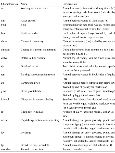
explain the cross section and time series of stock returns in the finance and accounting literature. The characteristics we choose include well-known drivers of stock returns such as beta, size, book-to-market, momentum, volatility, liquidity, investment and profitability. Table7 in the Appendix lists details of the
characteristics used and the methods to construct the data. We follow the procedures ofGreen et al.(2017) to construct the characteristics of interest. The characteristics used in our model are standardized to have
zero mean and unit variance. Figure 1 plots the histogram of monthly stock returns and9 standardized firm characteristics. Each of them have different distribution patterns, suggesting the potential nonlinear relationship between returns and firm characteristics, which can be potentially captured by our quantile
model.
Our empirical design is closely related to the characteristics model proposed by Daniel and Titman
(1997, 1998). To avoid any “data snooping” issue cause by grouping, we conduct the empirical analysis
[image:23.612.87.529.472.688.2]at individual stock level. Specifically, we use the sample period from January 2000 to December 2018, and estimate our model using monthly returns (228 months) from 1306 firms that have non-missing values during this period.
A “Characteristic + Latent Factor” Asset Pricing Model
We apply our model to fit the cross section and time series of stock returns ((Lettau and Pelger,2018)). There arenassets (stocks), and the return of the each asset can potentially be explained bypobserved asset
characteristics (sparse part) andr latent factors (dense part). The asset characteristics are the covariates in our model. Our model imposes a sparse structure on thep characteristics so that only the characteristics having the strongest explanatory powers are selected by the model. The part that’s unexplained by the firm
characteristics are captured by latent factors.
Suppose we have nstock returns (R1,...,Rn), and p observed firm characteristics (X1,...,Xp) overT
periods. The return quantile at levelτ of portfolioiin timetis assumed to be the following:
FR−1
i,t|Xi,t−1;θ(τ),λi(τ),gt(τ)(τ) =Xi,t−1,1θ1(τ) +...+Xi,t−1,kθk(τ) +...+Xi,t−1,pθp(τ)+ λi(τ) gt(τ)
(1×rτ) (rτ×1)
where Xi,t−1,k is the k-th characteristic (for example, the book-to-market ratio) of asset iin time t−1.
The coefficientθkcaptures the extent to which assets with higher/lower characteristicXi,t,kdelivers higher
average return. The termgtcontains therτ latent factors in periodtwhich captures systematic risks in the market, andλicontains portfolioi’s loading on these factors (i.e. exposure to risk).
There is a discussion in academic research on “factor versus characteristics” in late 1990s and early
2000s. The factor/risk based view argues that an asset has higher expected returns because of its exposure to risk factors (e.g. Fama-French 3 factors) which represent some unobserved systematic risk. An asset’s
exposure to risk factors are measured by factor loadings. The characteristics view claims that stocks have higher expected returns simply because they have certain characteristics (e.g. higher book-to-market ratios, smaller market capitalization), which might be independent of systematic risk (Daniel and Titman (1997,
1998)). The formulation of our model accommodates both the factor view and the characteristics view. The sparse part is similar to Daniel and Titman (1997, 1998), in which stock returns are explained by
firm characteristics. The dense part assumes a low-dimensional latent factor structure where the common variations in stock returns are driven by several “risk factors”.
Empirical Results
We first get the estimatesθˆ(τ)andΠ(ˆ τ)at three different quantiles,τ ={0.1,0.5,0.9}using our proposed ADMM algorithm. We then decomposeΠ(ˆ τ) into the products of its ˆrτ principal components ˆg(τ) and
their loadingsˆλ(τ)via eq(14). The(i, k)-th element ofˆλ(τ), denoted asλˆi,k(τ), can be interpreted as the
exposure of assetito thek-th latent factor (or in finance terminology, “quantity of risk”). And the(t, k)-th elements ofgˆ(τ), denoted as gt,kˆ (τ), can be interpreted as the compensation of the risk exposure to the
different tuning parametersν1andν2, and we use our proposed BIC to select the optimal tuning parameters.
The details of the information criteria can be found in equation (31).
The tuning parameter ν1 governs the sparsity of the coefficient vectorθ. The larger ν1 is, the larger
the shrinkage effect onθ. Figure2illustrate the effect of this shrinkage. Withν2 fixed, as the value ofν1
increases, more coefficients in the estimatedθvector shrink to zero. From a statistical point of view, the “effective characteristics” that can explain stock returns are those with non-zero coefficientθat relatively
[image:25.612.79.544.257.522.2]large values ofν1.
Figure 2: Estimated Coefficients as a Function ofν1
The figure plots the estimated coefficientθwhen the tuning parameterν1 changes, forτ ={0.1,0.5,0.9}.
The parameterν2is fixed atlog10(ν2) =−4.
Table3reports the relationship between tuning parameterν2 and rank of estimatedΠat different
quan-tiles. It shows that the tuning parameter ν2 governs the rank of matrix Π, and that as ν2 increases, we
penalize more on the rank of matrixΠthrough its nuclear norm.
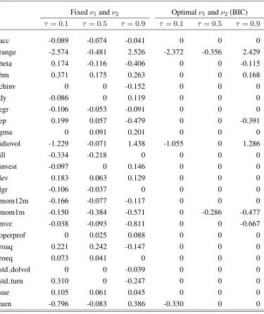
The left panel of Table 4reports the estimated coefficients in the sparse part when we fix the tuning parameters atlog10(ν1) =−3.5andlog10(ν2) =−4. The signs of some characteristics are the same across
the quantiles, e.g. size (mve), book-to-market (bm), momentum (mom1m, mom12m), accurals (acc), book
Table 3: The estimated rank ofΠ.
log10(ν2) τ = 0.1 τ = 0.5 τ = 0.9
-6.0 228 228 228
-5.5 228 228 228
-5.0 228 228 228
-4.5 164 228 168
-4.0 1 7 2
-3.5 1 1 1
-3.0 0 0 0
Note: Estimated under different values of turning
pa-rameterν2, whenν1 = 10−5is fixed. The results are
reported for quantiles 10%, 50% and 90%.
high beta stocks have high future returns, which is consistent with results found via the CAPM; while at
50%and 90% quantile, high beta stocks have low future returns, which conforms the “low beta anomaly” phenomenon. Volatility (measured by both range and idiosyncratic volatility) is positively correlated with future returns at 90% quantile, but negatively correlated with future returns at 10% and 50% percentile. The
result suggests that quantile models can capture a wider picture of the heterogenous relationship between asset returns and firm characteristics at different parts of the distribution (Koenker(2000)).
Table 5 reports the selected optimal tuning parameters ν1 andν2 for different quantiles. The tuning
parameters are selected via BIC based on (31) as discussed in Section5. For everyν1 andν2, we get the
estimatesθe(ν1, ν2) andΠ(e ν1, ν2) and the number of factorsr = rank(Π(e ν1, ν2)). Theθvector is sparse
with non-zero coefficients on selected characteristics. The 10% quantile of returns has only 1 latent factor,
and 3 selected characteristics. The median of returns has 7 latent factors and 2 selected characteristics. The 90% quantile of returns has 2 latent factors and 7 selected characteristics. Range is the only characteristic selected across all 3 quantiles. Idiosyncratic volatility is selected at 10% and 90% quantiles, with opposite
signs. 1-month momentum is selected at 50% and 90% percentiles, with negative sign suggesting reversal in returns.
Overall, the empirical evidence suggests that both firm characteristics and latent risk factors have
Table 4: Sparse Part Coefficients at Different Quantiles.
Fixedν1andν2 Optimalν1andν2(BIC)
τ = 0.1 τ = 0.5 τ = 0.9 τ = 0.1 τ = 0.5 τ = 0.9
acc -0.089 -0.074 -0.041 0 0 0
range -2.574 -0.481 2.526 -2.372 -0.356 2.429
beta 0.174 -0.116 -0.406 0 0 -0.115
bm 0.371 0.175 0.263 0 0 0.168
chinv 0 0 -0.152 0 0 0
dy -0.086 0 0.119 0 0 0
egr -0.106 -0.053 -0.091 0 0 0
ep 0.199 0.057 -0.479 0 0 -0.391
gma 0 0.091 0.201 0 0 0
idiovol -1.229 -0.071 1.438 -1.055 0 1.286
ill -0.334 -0.218 0 0 0 0
invest -0.097 0 0.146 0 0 0
lev 0.183 0.063 0.129 0 0 0
lgr -0.106 -0.037 0 0 0 0
mom12m -0.166 -0.077 -0.117 0 0 0
mom1m -0.150 -0.384 -0.571 0 -0.286 -0.477
mve -0.038 -0.093 -0.811 0 0 -0.667
operprof 0 0.025 0.088 0 0 0
roaq 0.221 0.242 -0.147 0 0 0
roeq 0.073 0.041 0 0 0 0
std dolvol 0 0 -0.039 0 0 0
std turn 0.310 0 -0.247 0 0 0
sue 0.105 0.061 0.045 0 0 0
turn -0.796 -0.083 0.386 -0.330 0 0
Note: The left panel reports the estimated coefficient vectorθin the sparse part for quantiles
10%, 50% and 90%, when the tuning parameters are fixed atlog10(ν1) =−3.5,log10(ν2) =
Table 5: Selected Optimal Tuning Parameters and
Number of Factors
τ = 0.1 τ = 0.5 τ = 0.9
optimalr 1 7 2
optimalν1 10−2.5 10−2.5 10−2.75
optimalν2 10−4 10−4 10−4
Note: This table reports the selected optimal tuning parameterν1andν2that minimize the objective
func-tion in equafunc-tion (31) for different quantiles.
Interpretation of Latent Factors
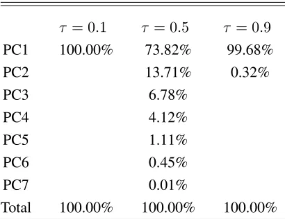
Table6below reports the variance in the matrixΠexplained by each Principal Component (PC) or latent factor. At upper and lower quantiles, the first PC dominates. At the median there are more latent factors
[image:28.612.203.408.429.587.2]accounting for the variations inΠ, with second PC explaining 13.8% and third PC explaining 6.8%.
Table 6: Percentage ofΠexplained by PC
τ = 0.1 τ = 0.5 τ = 0.9
PC1 100.00% 73.82% 99.68%
PC2 13.71% 0.32%
PC3 6.78%
PC4 4.12%
PC5 1.11%
PC6 0.45%
PC7 0.01%
Total 100.00% 100.00% 100.00%
Note: Variance of matrixΠexplained by each prin-cipal component for different quantiles.
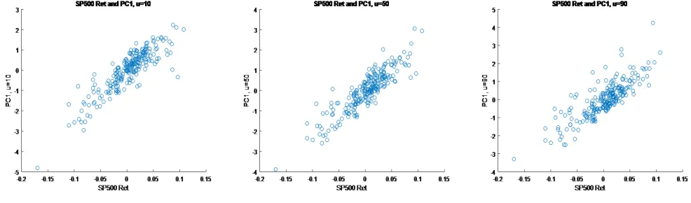
We also found the first PC captures the market returns in all three quantiles: Figure 3 plots the first principal component against the monthly returns of S&P500 index, showing that they have strong positive
Figure 3: The S&P 500 Index Return and the First PC at Different Quantiles.
This figure plots the first PC of matrixΠ against S&P500 index monthly return for quantiles 10% (left), 50% (middle), and 90% (right).
References
Jason Abrevaya and Christian M Dahl. The effects of birth inputs on birthweight: evidence from quantile estimation on panel data. Journal of Business & Economic Statistics, 26(4):379–397, 2008.
Alnur Ali, Zico Kolter, and Ryan Tibshirani. The multiple quantile graphical model. In Advances in Neural
Information Processing Systems, pages 3747–3755, 2016.
Tomohiro Ando and Jushan Bai. Quantile co-movement in financial markets: A panel quantile model with
unobserved heterogeneity. Journal of the American Statistical Association, pages 1–31, 2019.
Manuel Arellano and St´ephane Bonhomme. Quantile selection models with an application to understanding changes in wage inequality. Econometrica, 85(1):1–28, 2017.
Susan Athey, Mohsen Bayati, Nikolay Doudchenko, Guido Imbens, and Khashayar Khosravi. Matrix com-pletion methods for causal panel data models. 2018.
Jushan Bai. Panel data models with interactive fixed effects. Econometrica, 77(4):1229–1279, 2009.
Jushan Bai and Junlong Feng. Robust principal components analysis with non-sparse errors. arXiv preprint arXiv:1902.08735, 2019.
Jushan Bai and Kunpeng Li. Statistical analysis of factor models of high dimension. The Annals of Statistics, 40(1):436–465, 2012.
Jushan Bai and Serena Ng. Principal components estimation and identification of static factors. Journal of
Econometrics, 176(1):18–29, 2013.
Jushan Bai and Serena Ng. Principal components and regularized estimation of factor models. arXiv preprint
arXiv:1708.08137, 2017.
Alexandre Belloni and Victor Chernozhukov. On the computational complexity of mcmc-based estimators in large samples. The Annals of Statistics, 37(4):2011–2055, 2009.
Alexandre Belloni and Victor Chernozhukov. `1-penalized quantile regression in high-dimensional sparse
models. The Annals of Statistics, 39(1):82–130, 2011.
Peter Bickel, Ya’acov Ritov, and Alexandre Tsybakov. Simultaneous analysis of lasso and dantzig selector.
The Annals of Statistics, 37(4):1705–1732, 2009.
Stephen Boyd, Neal Parikh, Eric Chu, Borja Peleato, and Jonathan Eckstein. Distributed optimization and statistical learning via the alternating direction method of multipliers. Foundations and TrendsR in
Machine learning, 3(1):1–122, 2011.
Pratik Prabhanjan Brahma, Yiyuan She, Shijie Li, Jiade Li, and Dapeng Wu. Reinforced robust principal component pursuit. IEEE transactions on neural networks and learning systems, 29(5):1525–1538, 2017.
Jian-Feng Cai, Emmanuel Cand`es, and Zuowei Shen. A singular value thresholding algorithm for matrix completion. SIAM Journal on Optimization, 20(4):1956–1982, 2010.
John Campbell. Financial decisions and markets: a course in asset pricing. Princeton University Press, 2017.
Emmanuel Cand`es and Yaniv Plan. Matrix completion with noise. Proceedings of the IEEE, 98(6):925–936,
2010.
Emmanuel Cand`es and Yaniv Plan. Tight oracle inequalities for low-rank matrix recovery from a minimal number of noisy random measurements. IEEE Transactions on Information Theory, 57(4):2342–2359,
2011.
Emmanuel Cand`es and Benjamin Recht. Exact matrix completion via convex optimization. Foundations of
Computational mathematics, 9(6):717, 2009.
Emmanuel Cand`es and Terence Tao. The dantzig selector: Statistical estimation when p is much larger than n. The annals of Statistics, 35(6):2313–2351, 2007.
Gary Chamberlain and Michael Rothschild. Arbitrage, factor structure, and mean-variance analysis on large asset markets. Econometrica (pre-1986), 51(5):1281, 1983.
Sourav Chatterjee. Matrix estimation by universal singular value thresholding. The Annals of Statistics, 43 (1):177–214, 2015.
Liang Chen, Juan Dolado, and Jes´us Gonzalo. Quantile factor models. 2018.
Mingli Chen. Estimation of nonlinear panel models with multiple unobserved effects. Warwick Economics Research Paper Series No. 1120, 2014.
Mingli Chen, Iv´an Fern´andez-Val, and Martin Weidner. Nonlinear panel models with interactive effects.
arXiv preprint arXiv:1412.5647, 2014.
Victor Chernozhukov, Christian Hansen, and Yuan Liao. A lava attack on the recovery of sums of dense and
Victor Chernozhukov, Christian Hansen, Yuan Liao, and Yinchu Zhu. Inference for heterogeneous effects using low-rank estimations. arXiv preprint arXiv:1812.08089, 2018.
John H Cochrane. Asset pricing: Revised edition. Princeton university press, 2009.
John H Cochrane. Presidential address: Discount rates. The Journal of finance, 66(4):1047–1108, 2011.
Gregory Connor and Robert A Korajczyk. Risk and return in an equilibrium apt: Application of a new test methodology. Journal of financial economics, 21(2):255–289, 1988.
Arnak Dalalyan, Mohamed Hebiri, and Johannes Lederer. On the prediction performance of the lasso. Bernoulli, 23(1):552–581, 2017.
Kent Daniel and Sheridan Titman. Evidence on the characteristics of cross sectional variation in stock returns. the Journal of Finance, 52(1):1–33, 1997.
Kent Daniel and Sheridan Titman. Characteristics or covariances. Journal of Portfolio Management, 24(4):
24–33, 1998.
Andreas Elsener and Sara van de Geer. Robust low-rank matrix estimation. The Annals of Statistics, 46
(6B):3481–3509, 2018.
Eugene F Fama and Kenneth R French. Common risk factors in the returns on stocks and bonds. Journal of financial economics, 33(1):3–56, 1993.
Maryam Fazel. Matrix rank minimization with applications. 2002.
Guanhao Feng, Stefano Giglio, and Dacheng Xiu. Taming the factor zoo: A test of new factors. Technical report, National Bureau of Economic Research, 2019.
Junlong Feng. Regularized quantile regression with interactive fixed effects. arXiv preprint arXiv:1911.00166, 2019.
Antonio Galvao. Quantile regression for dynamic panel data with fixed effects. Journal of Econometrics, 164(1):142–157, 2011.
Antonio Galvao and Kengo Kato. Smoothed quantile regression for panel data. Journal of econometrics,
193(1):92–112, 2016.
Antonio Galvao and Gabriel V Montes-Rojas. Penalized quantile regression for dynamic panel data. Journal
of Statistical Planning and Inference, 140(11):3476–3497, 2010.
Domenico Giannone, Michele Lenza, and Giorgio Primiceri. Economic predictions with big data: The illusion of sparsity. 2017.
Stefano Giglio and Dacheng Xiu. Asset pricing with omitted factors. Chicago Booth Research Paper, (16-21), 2018.
Bryan S Graham, Jinyong Hahn, Alexandre Poirier, and James L Powell. A quantile correlated random
coefficients panel data model. Journal of Econometrics, 206(2):305–335, 2018.
Jeremiah Green, John Hand, and Frank Zhang. The characteristics that provide independent information