Canonical models of surfaces with K2 = 7 and pg = 4

(1)

warwick.ac.uk/lib-publications

A Thesis Submitted for the Degree of PhD at the University of Warwick

Permanent WRAP URL:

http://wrap.warwick.ac.uk/128955

Copyright and reuse:

This thesis is made available online and is protected by original copyright.

Please scroll down to view the document itself.

Please refer to the repository record for this item for information to help you to cite it.

Our policy information is available from the repository home page.

(2)

Canonical models of surfaces with

K

2

=

₇

_and

_p

g

=

4

by

Juan Salvador Garza Ledesma

Thesis

Submitted to the University of Warwick for the degree of

Doctor of Philosophy

Mathematics Institute

(3)

Acknowledgments

I am very grateful to Miles Reid for sharing with me with his deep understanding of algebraic geometry. Having had the opportunity of being his student has been the most inspiring and fun part of my academic life.

I am also grateful to Gavin Brown for his help during my first year at War-wick; to Stephen Coughlan, Ingrid Bauer and Fabrizio Catanese for their interest in my work and valuable suggestions during my visit to the University of Bayreuth; many thanks also to all the great people I met during my stance in KIAS, Seoul.

Last but not least, I want to express my gratitude to my examiners, Alessio Corti and Jan Stevens for their very useful comments and corrections.

(6)

Declarations

(7)

Abstract

Geometrically, the main goal of this thesis is to refine the classification of minimal surfaces S with K_S2 = 7 and p_g =4 due to Ingrid Bauer and published in

her monographSurfaces with K_S2 =7 and p_g =4 (cf. [Bauer]). She found that they

belong to 10 families according to the behaviour of the canonical map ϕKS. The

10 families form 3 irreducible components of moduli, but the details of how this happens remained unknown except for a few particular cases.

Our treatment consists in studying the abstract canonical model Proj R(S, K_S),

where R(S, KS) ∶= ⊕ n≥0

H0(S,O_S(nK_S)) is the pluricanonical ring. Except when ∣K_S∣is base point free, these rings are Gorenstein of codimension≥4. We show that

the only previously known deformation family of such rings (constructed by Bauer, Catanese and Pignatelli in [Bauer et al]) relating the 2 families withϕKS birational

can be recovered using basic arguments about halfcanonical curves. Our techniques also allow us to construct new explicit flat families for cases on which ϕKS is not

birational. In particular, we construct a 1-parameter flat family of Gorenstein rings with general fibre of codimension 4 and special fibre of codimension 6. At the end we discuss possible applications of our methods to the cases on which∣KS∣defines a

(8)

Chapter 1

Introduction and Preliminaries

This chapter introduces the notation and well known results used in the rest of the thesis. It also discusses the motivation leading to the geometric problems we are interested in.

1.1 Notation and conventions

The base field will always be the field of complex numbers C, most of the times

denoted simply by k.

A variety is an integral separated scheme of finite type over k; a curve is a variety of dimension 1, a surface is a variety of dimension 2, etc. Usually I will use the lettersC and S for referring to a curve and a surface respectively.

I will write Pn and An for the n−dimensional projective and affine spaces

overk. In this work however, the varieties will be more conveniently embedded in a weighted projective space (w.p.s.); the notationPn(wi₁1, . . . , w_sis), where ∑s_j₌₁ij = n+1, stands for the w.p.s. corresponding to the Proj of the ring k[x₀, . . . , x_n] with

its grading induced by thek×−action onkn+1∖ {0} given by

λ⋅ (a₀, . . . , a_n) ↦ (λw1a₀, . . . , λw1a_i₁, . . . , λwsa_n₊₁₋_i_s, . . . , λwsa_n).

Now, let X be a nonsingular variety, Y ⊂ X a nonsingular hypersurface, D, D1, D2 divisors on X and write O_X(⋅) for the corresponding invertible sheaf.

Then I write:

(9)

• H0(n₁D₁+n₂D₂) wheren₁, n₂∈_Z, as a short for H0(X,O_X(D₁)⊗n1 ⊗ O_X(D₂)⊗n2),

wheneverX is clear from the context.

• D∣Y or sometimes simplyDY for the restriction of the divisor DtoY. • In caseX=S is a surface, D₁D₂ denotes the intersection number. • In caseX=C is a curve, deg(D) denotes de degree of the divisorD. • hi(D) stands for the dimension ofH0(X,O_X(D))as a k−vector space. • χ(D)for the Euler characteristic of the sheafO_X(D), that is,∑n_i₌₀(−1)ihi(D). • ∣D∣for the linear system in which D moves.

• r(D) or simply r if there it is clear by the context, for the dimension of ∣D∣,

that is,h0(D) −1.

• ϕD for the rational map X ϕD

999K Pr, in case r≥1.

• g_dr for a linear system on a curve, of degree dand dimensionr.

• KX for a canonical divisor ofX.

• If X = S is a surface, I write p_g = p_g(S) = h0(K_S) for its geometric genus

and q = q(S) = h1(K_S) for its irregularity. If X = C is a curve, usually g = g(C) = h0(K_C) will denote its genus. Notice that Serre duality allows

us to define in an equivalent waypg =h2(O_S), q =h1(O_S) and similarly for

curves.

• R(X, D) stands for the full graded ring of sections of the divisorial sheaves O_X(nD):

R(X, D) ∶= ⊕ n≥0

H0(X,O_X(nD)).

In particular R(X, K_X) and R(X,−K_X) are called the canonical and

anti-canonical rings respectively. IfDis a divisor satisfying 2D∼K_X (Dis a theta

characteristic, semicanonical/halfcanonical divisor, etc.), the ring R(X, D) is called a halfcanonical ring onX.

• The notation Sa(x₁, . . . , x_n) stands for the set of monomials of degree a on

(10)

1.2 Basic facts and formulas

Here I state the results that will be used more frequently during the thesis. Since all of them are very well known, I omit giving any specific reference for their proofs. The reason for citing them is to make things clear afterwards, when I will simply writeby Clifford’s theorem, etc.

Theorem 1.2.1. (Riemann-Roch for curves) Let C be a nonsingular projective curve andD a divisor on it. Then

χ(D) =1−g+deg(D).

Remark The equality from previous theorem can be rewritten using Serre’s duality as:

h0(D) −h0(K_C−D) =1−g+deg(D).

Theorem 1.2.2. (Riemann-Roch for surfaces) Let S be a nonsingular projective surface andD a divisor on it. Then

χ(D) =χ(OS) +

1

2D(D−KS).

I will write simply R-R for referring to a Riemann-Roch theorem.

Theorem 1.2.3. (Adjunction formula) Let X ⊂Y be a nonsingular hypersurface

on a nonsingular variety. Then

KX = (KY +X)∣_X.

More generally, if Y is a Cohen-Macaulay variety and D is an effective Cartier divisor onY, then

ωD =ω_Y(D) ⊗ O_D

is a dualizing sheaf forD.

Corollary 1.2.4. If C⊂S is a nonsingular curve contained in a nonsingular

sur-face, then:

2g−2= (K_S+C)C

and the same is true for any curveC if we replace gfor the arithmetic genuspa(C). Theorem 1.2.5. (Bertini’s theorem)Let X be a nonsingular projective variety and

(11)

Theorem 1.2.6. (Castelnuovo’s base point free pencil trick) Let C be a smooth projective curve, Lan invertible sheaf on C and F a torsion free O_C−module.

Sup-pose that {s1, s2} is a linearly independent set of sections of L and denote byV the

subspace ofH0(C, L) it spans. Then the kernel of the cup-product map

V ⊗H0(C, F) Ð→H0(C, F ⊗L)

is isomorphic toH0(C, F⊗L−1(B)), whereB is the base locus of the pencil spanned

by s1 ands2.

Theorem 1.2.7. (Clifford’s theorem) Let C be a smooth projective genus g curve with an effective divisorD of degree d withd≤2g−1. Then

r(D) ≤d/2.

Moreover, if the equality holds, then either Dis zero, Dis a canonical divisor or C

is hyperelliptic andD is linearly equivalent to a multiple of a hyperelliptic divisor.

Remark A curve is called hyperelliptic if it admits a hyperelliptic divisor, that is, a divisor Dwith deg(D) =h0(D) =2.

Theorem 1.2.8. (Max Noether’s theorem)If C is not hyperelliptic, then the mor-phisms

Sym`H0(K_C) Ð→H0(`K_C)

are surjective for `≥1.

1.3 Classical Surface Theory background

LetS be a projective surface. Recall that theKodaira dimension ofS, denoted by

κ(S), is defined to be

κ(S) ∶= ⎧ ⎪ ⎪ ⎨ ⎪ ⎪ ⎩

Trk[R(S, KS)] −1 ifR(S, K_S) /≅k −∞ ifR(S, K_S) ≅k,

where Trk[R(S, KS)]is the transcendence degree (over_C) of the canonical ring.

(12)

Definition S is said to be a surface of general type ifκ(S) =2.

The next step in the classification is given by the following classic result:

Theorem 1.3.1. (Castenuovo’s contraction theorem) Let C ⊂ S be a curve on a

projective surface, such that C ≅_P1 and C2 = −1. Then there exists a nonsingular

surfaceS0 and a morphism

f ∶SÐ→S₀,

satisfying:

1. f(C) =P a point in S0.

2. f∶S∖ {C} Ð→S∖ {P} is an isomorphism.

So, the following definitions make sense:

Definition Keeping the notation from previous theorem: 1. C is said to be anexceptional curve of the first kind.

2. IfS is smooth and contains no exceptional curves of the first kind, then is said to be aminimal model.

The fact that every surface of general type can be obtained from a minimal model after blowing up a finite subset of smooth points, and moreover such minimal model is unique up to isomorphism, can be consulted in a number of well known references, (such as Chapter III, sections 4.4-4.6 of [BHPV]), and is one of the main guiding results on which the celebrated Minimal Model Program for varieties of higher dimensions is inspired.

Thus, classifying surfaces of general type leads to the study of the unique minimal model contained in each birational class. The most important numerical data associated to a minimal surface S is the triplet of integers formed by its geo-metrical genuspg, the irregularityq, and the self-intersection numberKS2. With the

exception ofK_S2, all of these are birational invariants.

Definition LetS be a minimal surface of general type. Thenumerical type of S is the triplet(K_S2, p_g, q).

(13)

1. The Euler characteristic of the structure sheaf is by definition:

χ(O_S) =1−q+p_g.

2. The topological Euler characteristic is (by a classical theorem of M. Noether):

e(S) =12χ(O_S) −K_S2.

3. The plurigeneraPm(S) ∶=h0(mK_S),m≥2 is (by R-R and Mumford’s

vanish-ing theorem):

Pm(S) =χ(OS) + (m

2)K

2

S.

For every minimal surface of general type S, there exists a unique normal surface X ⊂_PP5(S)−1 birational to S that is obtained contracting to points all the (−2)−curves of S (that is, curves E⊂S such thatE≅_P1 and E2= −2). Such an X

is called thecanonical model of S (cf. [Bombieri]) and in this context we know the following result:

Theorem 1.3.2.(cf.[Gieseker])There exists a quasi projective coarse moduli scheme for canonical models of surfaces of general type S with fixed K_S2 ande(S).

In practice, the approach is to fix a numerical type(K_S2, p_g, q) and consider

the subschemeM_K2

S,pg,qof the scheme whose existence is given by previous theorem. M_K2

S,pg,q is thus, a quasi projective scheme, in particular, it has finitely many

irre-ducible components. The ultimate goal in surface theory is to completely describe

M_K2

S,pg,q for as many numerical types as possible.

Remark (cf.[Debarre82],[Debarre83],[Miyaoka] and [Yau]) Of course there are re-strictions for the possible numerical type of a surface of general type; some well known inequalities involving these numbers are the following:

• K_S2 ≥1.

(14)

1.4 Previous work and statement of the problem

The case we want to attack were first seriously studied by Federigo Enriques in his famous book on algebraic surfaces [Enriques]. There he focuses on the effective construction of surfacesS, in particular, those withpg=4 and whose canonical map ϕKS is a birational morphism onto a singular surface Σ⊂P

3_{. The first open case,}

corresponding to K_S2 =7, has attracted the attention of several other

mathemati-cians besides Enriques himself; Franchetta ([Franchetta]), Maxwell ([Maxwell]) and Kodaira ([Kodaira]) to mention some.

Remark By Debarre’s inequality , it follows that ifSis a minimal surface of general type with pg = 4 and K_S2 = 7, then S is regular (that is, q = 0). Thus in the

subsequent, we will write simplyM₇_,₄∶= M_K2

s=7,pg=4,q=0for the corresponding moduli

space.

However, it was only until the beginnings of the 2000s when Ingrid Bauer, in her monograph [Bauer], gave a complete classification of surfaces inM₇_,₄, separating them into 10 families as stated in the following theorem (for a detailed version, consult Theorem 5.1, page 51 of [Bauer]):

Theorem 1.4.1. Let S be a smooth minimal surface withK_S2 =7and p_g=4. Then S belongs to exactly one of the following families:

• Family (0): ∣KS∣is base point free and the canonical mapϕ_K_S is a birational

morphism from S onto a surface of degree 7 in P3. These surfaces form an

open unirational, irreducible set of dimension 36 in the moduli spaceM7,4.

• Family (I): ∣KS∣ has exactly one simple base point P₁. Let π₁ ∶ ̃S Ð→S be

the blowup of S at P1 and let ∣ ̃H∣ be the movable part of ∣K_̃

S∣. Then we have

the following subfamilies:

– Family (I.1): ϕKS is a birational map. Then Σ ∶= ϕH̃( ̃S) ⊂ P

3 _{is a}

surface of degree 6 with the following properties: (a) The double curve Γ⊂Σis a plane conic.

(b) If γ⊂_P3 is the plane containing Γ, then Σhas a generalised tacnode o∈γ∖Γ with tacnodal plane α≠γ.

(c) ϕ_H_̃(E) = α∩γ, where E is the exceptional divisor of the blowup of P1∈S.

(15)

– Family (I.2): ϕKS is a map of degree 2 onto a cubic inP

3 _{that has only}

isolated singularities. These surfaces form an irreducible unirational set of dimension 33 inM₇_,₄.

– Family (I.3): ϕKS is a map of degree three onto a quadric inP

3_{. These}

surfaces also form an irreducible unirational set of dimension 35 inM7,4.

• Family (III): ∣K_S∣ has exactly three pairwise different simple base points P1, P2, P3∈S. Let π′∶ ̃S′Ð→S be the blowup ofS atP₁, P₂, P₃, let∣ ̃H′∣ be the

movable part of∣K_̃

S′∣ and let Ei ∶=π′−

1₍_P

i) be the exceptional divisors. Then

we have the following subfamilies:

– Family (III.α): ϕ_H_̃′( ̃S′) =_P1×_P1, (embedded in_P3 by the linear system ∣Γ₁ +Γ₂∣; where Γ₁2 = Γ2₂ = 0 and Γ₁Γ₂ = 1), and ϕ_H_̃′(E1), ϕ_H_̃′(E2), ϕ_H_̃′(E₃) are pairwise disjoint lines. These surfaces form an irreducible

unirational set of dimension 36 inM7,4.

– Family (III.β): ϕ_H_̃′( ̃S′) =_P1×_P1and without restrictionϕ_H_̃′(E1), ϕ_H̃′(E2) ≡

Γ1, ϕ_H̃′(E₃) ≡Γ₂. These surfaces form an irreducible unirational set of

dimension 38 in M7,4.

– Family (III.γ): ϕ_H_̃′( ̃S′) is the quadric cone. These surfaces form an

irreducible unirational set of dimension 35 inM₇_,₄ and they are obtained as degenerations of surfaces of family (III.α).

• Family (F): ∣K_S∣ has a non trivial fixed partF, with F2= −2 and K_SF =0.

Then, if∣H∣is the movable part of∣KS∣,∣H∣has exactly one simple base point X. Let π ∶ ̃S Ð→S be the blowup of S at X and let ∣ ̃H∣ be the movable part

of ∣K_S_̃∣. Then ϕ_H_̃ ∶ ̃S Ð→ Q is a morphism of degree 2 onto a quadric and ϕ_H_̃(F) is a line. We have the following 2 subfamilies:

– Family (F.1): ϕ_H_̃( ̃S) = _P1×_P1. These surfaces form an irreducible

unirational set of dimension 35 inM₇_,₄.

– Family (F.2): ϕ_H_̃( ̃S) is the quadric cone. These surfaces form an

irreducible unirational set of dimension 34 inM₇_,₄ and they are obtained as degenerations of surfaces of family (F.1).

• Family (F’):∣K_S∣ = ∣H∣ +F′and here the fixed part satisfiesF′2= −1,K_SF′=

1andHF′=2. In this case∣H∣is base point free andϕ_H(S) ⊂_P3is the quadric

cone. These surfaces form an irreducible unirational set of dimension 37 in

(16)

Remark In the above Theorem the roman digits indicate the number of base points of the canonical system ∣K_S∣, whereas the arabic numbers in the case (I) indicate

the degree of the canonical map.

By Kuranishi’s theorem (cf. [Kuranishi]), the dimension of the moduli space of all surfaces withK2=7 and p_g =4 in a generic point is at least 10χ−2K2=36.

Whence, the moduli spaceM7,4 has 3 irreducible components. There are two

com-ponents of dimension 36 that Bauer denotes byM₍₀₎and M₍_III.α₎. As the notation suggests, the components are the Zariski closure of the sets of surfaces of types (0) and (III.α) respectively. The third component, M₍_III.β₎, has dimension 38 and is

the Zariski closure of the set of surfaces of type(III.β).

The main result of Bauer concerning the moduli spaceM7,4 is the following:

Theorem 1.4.2. 1. The decomposition of the moduli space M₇_,₄ in irreducible components is:

M7,4=M₍₀₎∪M₍_III.α₎∪M₍_III.β₎.

2. The surfaces of type (III.γ) are contained in M₍₀₎∩M₍_III.α₎.

3. The two irreducible components M₍_III.α₎ and M₍_III.β₎ have empty intersec-tion.

Remark It follows that M7,4 has at most 2 connected components.

The next breakthrough came with the joint work of Bauer, Fabrizio Catanese and Roberto Pignatelli. By the results obtained previously by Bauer, it follows that is possible to find small deformations of surfaces in (I.1) falling into some of the big-ger pieces of moduli. In their paper [Bauer et al], they show how a surface in family (I.1) deforms into one in family (0). The main tool used to find such a deformation is the antisymmetric-extrasymmetric format, first discovered by Duncan Dicks and Miles Reid, when they studied surfaces withK2 =4 andp_g=3. This format is

use-ful for the presentation of certain Gorenstein rings of codimension 4 and has been used ever since many times to construct explicit deformation families of algebraic varieties. The format allows to deform the ring into one with codimension 3, which in our situation corresponds to a canonical surface of family (0). From the graded ring perspective, the difficulties in getting any other deformation and consequently a clearer picture ofM7,4 are the following:

(17)

(useful for family (0) of theorem 1.4.1) or the one given in [Bauer et al] (useful for family (I.1)) cannot be applied in any of the remaining cases.

2. Even if one manages to construct the pluricanonical ring, there are no formats that allow us to deform it if its codimension is greater than 4.

Thus, the main problem of this thesis is:

Problem 1.4.1. Can you obtain any other explicit deformation family of rings relevant to surfaces belonging to the cases described in Theorem 1.4.1?

1.5 Contents of the thesis

1.5.1 Main results

The main original contributions of this thesis are the following:

• (cf. Theorem 5.1.1). Consider the graded ringR∶=k[x₀, x₁, x₂, x₃, y₁, y₂, z]/I,

where degxi=1, degy_j =2, degz=3 andI is the homogeneous ideal generated

by 9 elements defined as follows: Let A ∶=

⎛

⎝

x1 x2 x3 y2

x2₂+a₁x₀x₂+a₂x2₀ Q y₁ z ⎞

⎠ ,

with Q ∶=x2₃+a₃x₁x₂+a₄x2₁+ (a₅x₁+a₆x₂+a₇x₃)x₀+a₈x2₀

and let M ∶= ⎛ ⎜ ⎜ ⎜ ⎜ ⎜ ⎝

Q₁ 1

2a19x 2

0 12(a20x0x2+a21x 2

0) 12a22x0 1

2a19x 2

0 Q2 1₂a27x20 12a28x0

1

2(a20x0x2+a21x 2

0) 12a27x 2

0 Q3 1₂a35x0

1 2a22x0

1 2a28x0

1

2a35x0 −1

⎞ ⎟ ⎟ ⎟ ⎟ ⎟ ⎠ , with ⎧ ⎪ ⎪ ⎪ ⎪ ⎪ ⎪ ⎪ ⎪ ⎨ ⎪ ⎪ ⎪ ⎪ ⎪ ⎪ ⎪ ⎪ ⎩

Q₁∶= a₉x2₁+a₁₀x₁x₂+a₁₁x₁x₃+a₁₂x2₂+a₁₃x₂x₃+a₁₄x2₃

+(a₁₅x₁+a₁₆x₂+a₁₇x₃)x₀+a₁₈x2₀,

Q₂∶= (a₂₃x₁+a₂₄x₂+a₂₅x₃)x₀+a₂₆x2₀,

Q₃∶= a₂₉x₁x₂+a₃₀y₁+ (a₃₁x₁+a₃₂x₂+a₃₃x₃)x₀+a₃₄x2₀.

The first 6 generators are the 2×2 minors ofAand the last 3 are the distinct

entries of the symmetric 2×2 matrix AM(TA). Then, for a general choice of

parameters ai ∈_C, 1 ≤i ≤35, R =R(S, K_S) where S is a surface of general

type withpg=4 andK2=7 whose canonical map is 2-to-1 onto a cubic surface

(18)

• In Theorem 5.1.3 we prove that the rings described in the above result are degenerations of canonical rings of surfaces in the stratum (I.1).

• In Section 5.2 we give a new and simpler proof of the main result obtained by Bauer, Catanese and Pignatelli in their paper [Bauer et al]. That is, every surface in stratum (I.1) can be obtained as a degeneration of a surface in stratum (0).

• Let₍̃_I.₃₎ _{be the stratum formed by surfaces defined as Proj} _R _where _R _{is a}

ring of the form:

R∶=k[x₀, x₁, x₂, x₃, y₁, y₂, y₃, z₁, z₂]/I,

withxi,yj and z` of degrees 1, 2 and 3 respectively. P is the degree 4

homo-geneous form:

P ∶=a₁x3₀x₂+x2₀A₀+x2₁A₁+x₂2A₂+x2₃A₃+x₁x₂B₁+x₂x₃B₂, (1.1)

where

A0∶=a₂x2₁+a₃x₁x₂+a₄x₁x₃+a₅x2₂+a₆x₂x₃+a₇x2₃,

A1∶=a₈x₀x₁+a₉x₀x₂+a₁₀x2₁+a₁₁x₁x₂+a₁₂x2₂+a₁₃y₁+a₁₄y₂+a₁₅y₃,

A2∶=a₁₆x₀x₁+a₁₇x₀x₂+a₁₈x₀x₃+a₁₉x₁x₂+a₂₀x₁x₃+a₂₁x₂x₃+a₂₂x2₃+a₂₃y₃,

A3∶=a₂₄x₀x₂+a₂₅x₀x₃+a₂₆x₂x₃+a₂₇x2₃+a₂₈y₃

B1∶=a₂₉y₂+a₃₀y₃,

B2∶=a₃₁y₃,

a1, . . . , a31∈_C andI is generated by the 2×2 minors of ⎛

⎜ ⎜ ⎜ ⎝

x1 x2 y1 y2 z1

x2 x3 y2 y3 z2

y1 y2 z1 z2 P

⎞ ⎟ ⎟ ⎟ ⎠ .

Then every surface in₍̃_I.₃₎_{has a small deformation to either a surface in}₍_I.₃₎

or(I.1) (cf. §6.3 and Theorem 6.3.2).

If we make the following definition (cf. §2.3):

(19)

1. If I write(⋆) Ð→ (●), I mean that there exists a flat family with base a small

disc ∆t⊂ _C whose special fibre is of type ●, whose general fibre is of type ⋆

and this family exists for every point of a stratum●.

2. If I write(⋆) (●), I mean that there exists a flat family with base a small

and this family exists only for some points of a stratum●.

Our main results together with the conjectures made in the last chapter of this thesis lead to the following diagram:

(I.2) (̃I.3) (I.3)

(III.γ) (I.1)

(III.α) (0) (III.β)

(F.2) (F.1) (F′)

Here, the purple arrows are conjectured to exist, whereas the 3 different colours of names of the strata indicate the irreducible component of the moduli space they belong to (cf. §7.1).

1.5.2 Brief description of the chapters

• Chapter 2 describes Reid’s approach to the problem. In short terms, Reid’s philosophy is that studying surfaces is, because of the hyperplane section prin-ciple, closely related to the study curves and threefolds. If one is to find the deformations mentioned in Problem 1.4.1, one should study the canonical ring

R(S, K_S), whose algebraic structure is closely related with that of the

half-canonical ringR(C, KS∣_C), where C∈ ∣K_S∣is a canonical curve.

(20)

• In Chapter 4, I deal with the cases (I.3) and (III), whose corresponding Goren-stein rings have codimension 6 and 8, respectively. The algebra of these rings is much more subtle than that of those studied in previous chapter, but sur-prisingly, the geometry of the curves/surfaces is somewhat simpler and allows us to compute the rings by restricting sections of certain toric key varieties.

• Chapter 5 discusses explicit deformations of surfaces of types (I.1) and (I.2); both subfamilies can be studied as Proj of Gorenstein codimension 4 rings that extend the formats found in the curve case. In particular, we see that the result of Bauer, Catanese and Pignatelli can be obtained starting from a halfcanonical ring of a curve and then using the extension algorithm.

• In Chapter 6, it is shown that all the formats obtained in Chapter 4 for the halfcanonical rings of curves in the canonical system of surfaces of subfamily (I.3) extend to the surface case. These rings are Gorenstein codimension 6, related by 20 equations yoked together in 64 syzygies and are rather compli-cated.

• In the final Chapter we discuss a plausible strategy for treating the cases on which the canonical system defines a 2-to-1 map to a quadratic surface. The method is analogous to that used in previous chapter to deform the codimen-sion 6 rings. The rings involved here have codimencodimen-sion 8 and although working explicitly with them is naturally much more complicated, we believe that we will be able to answer important questions about the connectedness of the moduli space of surfaces withK2=7 andp_g=4 in the near future. In fact we

conjecture that the moduli space is connected and provide some experimental evidence suggesting this.

• Appendix This thesis contains a series of computer algebra codes that are sanity checks needed in several parts of the text. All of them can be run in Magma Online Calculator (cf. [BCP-Magma]):

http://magma.maths.usyd.edu.au/calc

In addition they can be found in my personal website:

(21)

Chapter 2

The Graded Ring Program

Reid’s suggestion to study problems on minimal surfaces of general type, is to look at the deformations of their canonical rings. His program was carried out by Dun-can Dicks in his PhD thesis [Dicks] for surfaces withK_S2 =4 and p_g=3 and shortly

later explained in detail in his article [Reid D-E], where he applied it to study de-formations of Horikawa quintics and also set the challenge of applying his methods to cases corresponding to higher values ofK_S2 and pg.

This fits in the framework of the more general and ambitious Graded Ring Program; starting with a polarised varietyX, L, one follows Zariski’s standard con-struction of the graded ring R(X, L) = ⊕

n≥0

H0(X, nL) which in many interesting

cases, turns out to be a Cohen-Macaulay, or even better, a Gorenstein ring. Know-ing how to construct a rKnow-ingR(X, L) by giving a presentation (that is by generators

and relations), can be achieved by combining algebro-geometric techniques depend-ing on the particular choice of the pair(X, L)and gives precise answers to questions

not only on embedding X ↪ _Pn and determining the equations of the image but

also, if the presentation obtained is good enough, on the deformation families of such rings/varieties. The worked example 2.4 illustrates many features of the program in an elementary case.

A couple of general conventions about the graded rings R that we will be working with are the following:

1. Graded rings will beN−graded, that is, R= ⊕ n≥0

Rn.

(22)

3. We do not require R to be generated over k by R1. Geometrically this

im-plies that in general, our varieties will be embedded in a weighted projective space, algebraically this implies that the codimension (and hence the number of equations defining the variety) remains small.

2.1 Gorenstein rings

For the purposes of this thesis, I can use the next definition of Gorenstein rings (for a more detailed discussion see [Reid 4], §1.1):

Definition Let I ⊂ O be a graded ideal in a regular graded ring. Let R = O/I.

Consider a minimal free resolution with gradedO−modules:

R←R₀←R₁← ⋯ ←R_c₋₁ ←R_c←0 (2.1)

Then R is a Cohen-Macaulay ring if c = codim_OI. If R is Cohen-Macaulay and Rc≅ O(−`)for some`∈_Z, then R is aGorenstein ring.

Remark IfR is Gorenstein, in particular one has a pairing on the resolution (2.1),

R∨_c₋_i(−`) ≅R_i coming from Serre duality.

In our context, R is of the form R(X, L) with X a variety and L and

ample Cartier divisor and the following result gives a characterisation of Cohen-Macaulay and Gorenstein rings that can be taken as an alternative definition (cf. [Hartshorne DT], Proposition 8.6).

Proposition 2.1.1. Consider the graded ring R(X, L) = ⊕ n≥0

H0(X, nL), with X a

projective variety andL an ample Cartier divisor. Then: 1. R is Cohen-Macaulay if and only if:

(a) hi(X, nL) =0 for all n and every iwith 0<i<dimX,

(b) h0(X, nL) =0 for all n<0,

(c) hdimX(X, nL) =0 for n≫0.

2. R is Gorenstein if and only if it is Cohen-Macaulay and KX = `L for some `∈_Z.

The following is an immediate consequence of the above criterion, the remark in section§ 1.4 and Kodaira vanishing theorem:

Corollary 2.1.2. LetS be a minimal surface of general type with invariantsK_S2 =7

(23)

2.1.1 Structure theorems

There are general structure theorems for Gorenstein rings in codimensions 2, 3 and 4 (by Serre, Buchsbaum-Eisenbud and Reid respectively) that we briefly recall next.

• In codim 2, Serre proved every Gorenstein ring is a complete intersection (see [Serre]).

• Codimension 3 is the easiest case we will find in this thesis, and the structure theorem is given by Buchsbaum and Eisenbud in [Buchsbaum-Eisenbud]. The result states thatR= O/I is a Gorenstein ring of codim 3, if and only if it has

a minimal free resolution of the form

R← O ← O2m+1 φ

←Ð O2m+1← O ←0, (2.2)

withφ given by a skew (2m+1) × (2m+1) matrix whose 2m×2m Pfaffians

generateI. In most of the cases occurring in practice (and in particular in the ones we will find in this thesis) it turns out that m=2 works. For this and

further purposes, it is convenient to introduce some notation for 4×4 Pfaffians

and skew matrices:

We will always omit the diagonal of zeroes and lower triangular antisymmetric block of any skew matrix appearing in this thesis, so for example, a skew 5×5

matrix will be written as

φ= ⎛ ⎜ ⎜ ⎜ ⎜ ⎜ ⎝

a12 a13 a14 a15

a23 a24 a25

a34 a35

a45

⎞ ⎟ ⎟ ⎟ ⎟ ⎟ ⎠

(2.3)

And we will write Pfi(φ)for the Pfaffian of the 4×4 submatrix obtained after

deleting the ith row and column of φ. So, Buchsbaum-Eisenbud result says that in casem=2, following above notation, the generators of I are (modulo

plus/minus signs):

Pf1(φ) =a₂₃a₄₅−a₂₄a₃₅+a₂₅a₃₄,

Pf2(φ) =a₁₃a₄₅−a₁₄a₃₅+a₁₅a₃₄,

Pf3(φ) =a12a45−a₁₄a₂₅+a₁₅a₂₄,

Pf4(φ) =a₁₂a₃₅−a₁₃a₂₅+a₁₅a₂₃,

Pf5(φ) =a₁₂a₃₄−a₁₃a₂₄+a₁₄a₂₃.

(24)

More generally, if we take M, a skew m×m matrix with m ≥6 and entries Mr,swe will denote simply byij.k`, wherei<j<k<`, the Pfaffian of the 4×4

matrix obtained by picking 4 rows and the corresponding columns according to the index selection. More precisely:

ij.k`=M_ijM_k`−M_ikM_j`+M_i`M_jk. (2.5) • Reid’s codimension 4 structure theorem given in [Reid 4],§2.5, is an analogous result to that of Buchsbaum-Eisenbud in codimension 3, however, as stated there, in terms of certain key varieties called Spin-Hom varieties, is still far from being applicable in practice. As a substitute, we will be using certain ad-hoc methods for computing each of the codim 4 or higher Gorenstein rings that we find during the thesis.

2.1.2 Rolling factors

Throughout the thesis, we will come up with rings admitting a presentation that we will say to be inrolling factors format. Although we will emphasise on this later on, we include the definitions here for convenience of the reader.

LetI be an ideal in a polynomial ringO. Suppose that there exists a matrix A∈Mat₂_,n(O),

A= ⎛

⎝

f11 f12 . . . f1n f21 f22 . . . f2n

⎞

⎠

such that its(n₂)two by two minors are inI. We say that an element r₍n

2)+1

∈I can

be rolled with respect to the matrixAif it is in the ideal generated by the elements of its first row. Sor₍n

2)+1 is of the form

r₍n

2)+1

= n ∑ i=1

aif1i for someai ∈ O.

We call

r₍n

2)+2

∶= n ∑ i=1

aif2i

a rolling of r₍n

2)+1 with respect to A. If r(

n

2)+2

∈ I and it can be rolled again with

respect to A, we say that r₍n

2)+1 can be rolled twice, etc. Finally if I is finitely

generated and its remaining generators r₍n

2)+2, . . . , r(

n

2)+m are successive rollings of

r₍n

(25)

2.1.3 The hyperplane section theorem

Gorenstein rings are well behaved under taking hyperplane sections. The general philosophy as mentioned before is that the algebro-geometric properties of a ring/variety are closely related to those of its hyperplane sections. The main ingredient forma-lising these ideas is the following result:

Theorem 2.1.3. (The hyperplane section principle) LetR be a graded ring, letRd

be the degree d component (g ≥ 1), and let x₀ ∈ R_d be a non zero divisor. There

exists an exact sequence

0→R(−d) x0

Ð→R π

Ð→R∶=R/(x₀) →0. (2.6)

And we have:

1. If x1, . . . , xn ∈R generate R and x₁, . . . , x_n ∈ R are such that π(x_i) = x_i for

1≤i≤n. Then x₀, x₁, . . . , x_n generate R.

2. Suppose

R≅k[x₁, . . . , x_n]/(f₁, . . . , f_m). (2.7)

Then there exists relationsF1, . . . , Fm holding betweenx0, x1, . . . , xn, such that π(Fi) =f_i and F_i generate the idealkerev, where

ev∶k[x₀, . . . , x_n] →R. (2.8)

3. Similarly for syzygies, that is, if we have a syzygyσi∶ ∑m_j₌₁ljfj ≡0∈k[x₁, . . . , x_n].

Then there are Lj∈k[x₀, . . . , x_n] such that the following syzygy holds:

Σi∶ m ∑ j=1

LjFj ≡0∈k[x₀, . . . , x_n], (2.9)

(26)

Proof. Consider the diagram

0 0

J I

0 (x0) k[x₀, . . . , x_n] k[x₁, . . . , x_n] 0

0 R(−d) R R 0

0

x0 π

(2.10)

where the two horizontal sequences are exact and the dashed arrow is the unique morphism making the diagram commute. Letf x0 ∈ (x₀). Under the dashed

mor-phism, f x0 maps to f ∈ R_deg₍_f₎ = R(−d)_deg₍_{f x}

0). This morphism is well defined

becausex0 is a non zero divisor (i.e.,(x0) ⊂R is a freeR−module). Moreover it is

an isomorphism. Then it follows from the snake lemma that

k[x0, . . . , xn] →R (2.11)

is surjective. In other words, R is generated by x0 and the preimages ofx1, . . . , xn

under π. It follows also that I ≅ J as modules over k[x₀, . . . , x_n]. Suppose that f1, . . . , fm are generators of I over k[x₁, . . . , x_n], then f₁, . . . , f_m are generators

of I over k[x₀, . . . , x_n]. Therefore there exist F₁, . . . , F_m that generate J over k[x₀, . . . , x_n]. Now, notice that the isomorphismJ Ð→ I≅ is simply the restriction of k[x0, . . . , xn] →k[x₁, . . . , x_n], which is uniquely determined by x_i↦x_i for 1≤i≤n,

andx0↦0.

Finally, letFj =f_j+x₀g_j for someg_j ∈k[x₀, . . . , x_n]. Suppose σ_i∶ ∑mj=1ljfj ≡

0. Then

m ∑ j=1

ljFj ≡x₀ m ∑ j=1

ljgj. (2.12)

Since ∑m_j₌₁ljFj ∈ J and x₀∑m_j₌₁ljgj ∈ (x0) which, because x₀ is a non zero divisor,

implies ∑m_j₌₁ljgj ∈ J, we can write ∑m_j₌₁ljgj = ∑m_j₌₁hjFj. Thus Σi ∶ ∑m_j₌₁LjFj ≡0,

(27)

2.2 Extension algorithm

This section goes trough Reid’s extension theory that is clearly explained in [Reid D-E] and Dicks’ practical approach to it.

LetS be a surface in M7,4. Roughly speaking, the hyperplane section

theo-rem says that the generators, relations and syzygies ofR(S, K_S) occur in the same

degrees of those ofR(C, D), whereC∈ ∣KS∣andD=K_S∣_C. Because of the geometry

of curves tends to be more tractable than that of surfaces, we will start computing

R(C, D). Suppose we find a presentation:

R(C, D) ≅k[x₁, . . . , x_n]/I; whereI = (f₁, . . . , f_m) (2.13)

Together with syzygies

σi∶ m ∑ j=1

ljfj ≡0. (2.14)

Then we should aim to find

Fj =f_j+x₀f_j′+x₀f_j′′+ ⋯ +x`₀f_j(`)+ ⋯ (2.15)

such thatf_j(`)∈k[x₁, . . . , x_n], and the F_j satisfy the syzygies Σ_j of theorem 2.1.3,

part 3, so we produce the sequence

{R(C, D)},{R(2C, D(2))}, . . . ,{R(dC, D(d))},{R(S, K_S)} (2.16)

by calculating Fj in stages allowing successively higher powers of x0. Each R((`+

1)C, D(`+1)) depends in a linear way onR(`C, D(`)) and we have

{R((`+1)C, D(`+1))/(x`₀)} ⊂ {R(`C, D(`))}. (2.17)

The following definitions are given to show in greater detail how this gets done:

Definition Suppose we have

R(C, D) ∶=R(1)≅k[x₁, . . . , x_n]/I (2.18)

and

(28)

such thatR(`) modulo x0 isR(1).

1. Define SR to be the graded k[x₁, . . . , x_n]−module with grading [S_R]_δ =R(1) δ−1

and multiplication defined by

f g=0 for all f, g∈S_R. (2.20)

2. Define T_R(`) to be the graded k[x₀, . . . , x_n]−module with grading [T_R(`)]_δ = [R(`)]_δ and multiplication defined by

( `−1

∑ i=0

xi₀pi) ( `−1

∑ i=0

xi₀qi) =x₀ `−2

∑ i=0

xi₀ ∑ j+s=1

pjqs, (2.21)

for all

`−1

∑ i=0

xi₀pi, `−1

∑ i=0

xi₀qi∈T_R(`).

Then we have the following result (cf.[Lichtenbaum-Schlessinger],§4.2.5):

Proposition 2.2.1. With R(1) andR(`) as above,R(`+1) exists if and only if there exists a degree preserving module homomorphism β` as shown in the following

dia-gram, withβ`○ι′_`=α′_`.

0 Σ (f₁, . . . , f_m) k[x₁, . . . , x_n] R(1) 0

0 SR TR(`) R(`) R(1) 0 ι′_`

α′_` β` α`

ι` j`

(2.22)

The rows of 2.22 are exact. Σis the k[x₁, . . . , x_n]−module generated by the syzygies σ1, . . . , σt such that the top row is exact. The maps ι` andj` are given by

ι`(p) =x`0−1p,

j`( `−1

∑ i=0

xi₀pi) =x₀ `−2

∑ i=0

xi₀pi.

(2.23)

The mapsα`andα′`of previous diagram are defined inductively, they depend

on the mapβ`−1 defined by an analogous diagram as we will see:

(29)

0 Σ (f₁, . . . , f_m) k[x₁, . . . , x_n] R(1) 0

0 SR TR(1) R(1) R(1) 0

ι′

α′₁ β1 α1

ι j

(2.24)

Where the mapsα1, α′1 and j are all zero, andι is the identity map. We must find

β1∶ I = (f₁, . . . , f_m) Ð→S_R, (2.25)

such that degβ1(fi) =degf_i−1 and m ∑ i=1

liβ1(fi) =0 wheneverι′(σ_j) = m ∑ i=1

lififor some σj. The fact this problem always has a solution (namely the zero map), corresponds

to the fact that first order extensions are alwaysunobstructed. The construction of

β1 allows us to define

R(2)(β₁) =k[x₀, . . . , x_n]/(I(2), x2₀), (2.26)

whereI(2) is generated by F₁, . . . , F_m given by F_i=f_i+x₀β₁(f_i).

To go from ring R(2) to R(3), take any map β ∶ (f1, . . . , fm) →S_R such that β(f₁), . . . , β(f_m) are generic polynomials making the above conditions hold. Then

this map can be lifted to ˜

β∶ I Ð→k[x₁, . . . , x_n], (2.27)

where

m ∑ i=1

liβ˜(f_i) ∈ I whenever ι′(σ_j) = m ∑ i=1

lifi for someσj.

Then α2 ∶ I → T_R(2) is given by α₂(f_i) = β(f_i). Consider σ_j such that ι′(σ_j) =

m ∑ i=1

lifi, then the first step has given the expression m

∑ i=1

liβ˜(f_i) = m ∑ s=1

psfs∈ I. (2.28)

We defineα′₂(σj) ∶= m ∑ s=1

(30)

0 Σ (f₁, . . . , f_m) k[x₁, . . . , x_n] R(1) 0

0 SR TR(2) R(2) R(1) 0

ι′₂

α′₂ β2 α2

ι2 j2

(2.29)

must satisfy

m ∑ i=1

liβ2(f_i) = m ∑ s=1

psβ(f_s) and as in the first step, the construction ofβ₂

allows us to put

R(3)(β₂) =k[x₀, . . . , x_n]/(I(3), x3₀), (2.30)

whereI(3) is generated by {F₁, . . . , F_m}given by

Fi =f_i+x₀β(f_i) +x2₀β₂(f_i). (2.31)

If there are no mapsβ2 making diagram 2.29 commute, we say the extension

isobstructed; when this happens, we will be forced to impose further conditions on the generalβ to make the diagram commute.

The above procedure continues inductively when getting fromR(`)toR(`+1), the presence of obstructions makes clear why in general

{R((`+1)C, D(`+1))/(x`₀)} ⫋ {R(`C, D(`))}. (2.32) Remark In practice, it is often possible to save a lot of time and effort by doing some simplifications at each step and using the concept offlexible formats to write the generators ofI; this is explained later on in Chapter 5. Besides the worked

ex-ample at the end of this chapter, the reader is also encouraged to consult Pinkham’s example, that can be found in [Reid D-E],§2.1.

2.3 The Main Set up

LetS be a minimal surface with K_S2 =7 andp_g=4. Let ∣H∣be the movable part of ∣K_S∣. For convenience of the reader, I summarise the classification given in Theorem

(31)

Family Base locus of ∣KS∣ Brief description of ϕ_H

(0) None Birational to a surface of degree 7. (I.1) One base point Birational to a surface of degree 6. (I.2) One base point 2-to-1 to a cubic surface.

(I.3) One base point 3-to-1 to the quadric cone. (III.α) Three base points 2-to-1 to_P1×_P1.

S admits a genus 2 pencil.

(III.β) Three base points 2-to-1 to_P1×_P1.

S does not admit a genus 2 pencil.

(III.γ) Three base points 2-to-1 to the quadric cone. (F.1) F withF2= −2 2-to-1 to_P1×_P1.

and KSF =0

(F.2) F withF2= −2 2-to-1 to the quadric cone.

and KSF =0

(F′) F′ with F′2= −1, 2-to-1 to the quadric cone. KSF′=1 andHF′=2

Definition Let(⋆)and(●)be two families of surfaces according to the classification

of Theorem 1.4.1.

1. If I write(⋆) Ð→ (●), I mean that there exists a flat family with base a small

and this family exists for every point of a stratum●.

2. If I write(⋆) (●), I mean that there exists a flat family with base a small

and this family exists only for some points of a stratum●.

For example, the only known situation coming from explicit deformation of canonical rings was obtained in the work of Bauer, Catanese and Pignatelli [Bauer et al] and is:

(0) Ð→ (I.1).

However, by easy geometric arguments, the structure of the moduli space for the cases in which∣K_S∣has a non-trivial fixed part is almost completely understood.

(32)

(III.α)

(III.γ) (F.1)

(F.2)

(III.β)

(F′)

(2.33)

The above considerations suggest us to focus in the cases in which the cano-nical system has no fixed part. Guided also by the hyperplane section principle, we propose the following Main Setup:

• In the subsequent, unless otherwise stated,S will denote a minimal surface of general type withK_S2 =7,p_g =4 and such that∣K_S∣has no fixed part.

• C∈ ∣K_S∣will be a general canonical curve that can be assumed to be

nonsin-gular; because of Bertini’s theorem and because it is known that∣KS∣can only

have simple base points.

– Letg be the genus of C. By the adjunction formula, 2g−2=2K_S2, thus g=8.

– Dwill denote the restrictionKS∣_C. So, again by adjunction,K_C =2K_S∣_C,

thereforeD is a degree 7 halfcanonical divisor.

– Since pg = 4 and the surfaces we are considering are regular, it follows

thath0(D) =3, soD moves in ag₇2.

As expected, there are exactly 5 general possibilities for a divisorD∈g₇2, namely:

1. ∣D∣has no base points.

2. ∣D∣ has exactly one base point P. Let D′ ∶=D−P, then ϕ_D′ ∶C Ð→_P2 is a

degree 6 morphism and one has 3 sub cases: (a) ϕD′(C) is a sextic with 2 double points.

(b) ϕD′(C) is an elliptic curve.

(c) ϕD′(C) is a plane conic

3. ∣D∣has exactly 3 base pointsP₁, P₂, P₃. LetD̃∶=D−P₁−P₂−P₃ soϕ_D_̃∶CÐ→

P2 is a degree 4 morphism. In this case the only possibility for ϕD̃(C) is to

(33)

Remark • The above possibilities are obtained as easy numeric consequences, following from the factorisations 6 = 2×3, 4 = 2×2 and the degree-genus

formula (or adjunction formula).

• It can be shown that the sextic in the general case corresponding to 2.(a) is tangent to the line joining its two singular points.

• In case 2.(c), because of the rationality of the conic, it follows that C is a trigonal curve (that is, is non hyperelliptic curve admitting ag₃1).

• Similarly it follows that any curve in case 3 is a hyperelliptic curve.

Our task during the following two chapters will be to computeR(C, D) for

a polarised curve falling in each of the cases above.

2.4 Worked Example

Let C be a nonsingular projective curve of genus g(C) = h1(O_C) = 2. Assuming

Riemann-Roch for curves holds, my aim is then to studyC as an abstractly given object, by means of the graded rings R(C, D) with respect to certain polarising

ample divisorD.

2.4.1 Canonical and bicanonical rings on a genus 2 curve

First consider the canonical classKC. By R-R and Serre duality: h0(K_C) =deg(K_C).

This is the well known fact that every genus 2 curve is hyperelliptic, and

∣KC∣ =g₂1. It defines a morphism

π∶=ϕ_K_C ∶C

2-to-1

ÐÐÐ→_P1,

branched, by Riemann-Hurwitz formula, at 6 (necessarily distinct, since C is non-singular) pointsBi∈_P1, 1≤i≤4. This leads to the model of C as a hypersurface

in weighted projective space (w.p.s.)

P(1,1,3) =Projk[t₁, t₂, u];

we have

(34)

where f6 is a homogeneous degree 6 form in t1, t2 whose zeroes define the branch

locus. For illustrative purposes, I take

f6(t₁, t₂) =t6₁−t₁t5₂. (2.35)

This is an example of a codimension 1 Gorenstein ring; you can deduce the presentation (2.34) in any number of ways, perhaps the easiest being simply to follow the corresponding Riemann-Roch table (which is explained just below):

Space Dimension Generators Relations

H0(C, KC) 2 t₁, t₂ None

H0(C,2K_C) 3=2 deg(K_C) −1 S2(t₁, t₂) None H0(C,3K_C) 5=3 deg(K_C) −1 S3(t₁, t₂),u None H0(C,4K_C) 7=4 deg(K_C) −1 S4(t₁, t₂),S1(t₁, t₂) ⊗u None H0(C,5KC) 9=5 deg(K_C) −1 S5(t₁, t₂),S2(t₁, t₂) ⊗u None H0(C,6K_C) 11=6 deg(K_C) −1 S6(t₁, t₂),S3(t₁, t₂) ⊗u,u2 u2−t6₁−t6₂ H0(C, nK_C) 2n−1 Sn(t₁, t₂),Sn−3(t₁, t₂) ⊗u None

Let {t1, t2} be a basis of H0(K_C). Then Sn(t₁, t₂), n ≥ 2 gives us n+1

linearly independent sections ofH0(nK_C), because any relation would imply that ϕKC(C) ⊂ P

1 _{is reducible. Now, by Riemann-Roch I only need the 3 elements of}

S2(t1, t2) to get a basis of H0(2K_C), however in degree 3, I need a new generator, u, because h0(3K_C) = 5 and I only have the 4 linearly independent elements from S3(t₁, t₂).

Next, observe that there is no relation holding between elements ofS4(t₁, t₂)

and u⊗S1(t₁, t₂), because they belong to different factors of the decomposition of π_∗O_C in±eigensheaves: O

P1⊕ OP1(−3). Therefore the 7 elements inS

4₍_t

1, t2) ∪u⊗ S1(t₁, t₂) form a basis of H0(4K_C). For similar reasons, it follows that there are

no relations between elements ofSn(t1, t2) andu⊗Sn−3(t₁, t₂)for anyn≥4. Thus,

the only relation occurs in degree 6, and the coefficient of u2 must be non-zero. After completing the square and possibly changing coordinates, we get the desired presentation.

Previous computation gives for free a presentation of thebicanonical subring

R(C,2KC) = ⊕ n≥0

(35)

This is a codimension 3 Cohen-Macaulay ring and the following statements are easy consequences of the presentation we obtained of the canonical ringR(C, D):

1. There is a mapϕ2KC ∶C

2-to-1

ÐÐÐ→C⊂_P2, whereC≅_P1 is a nonsingular conic.

2. R(C, D) is generated in degree 2 and related in degree 4; in detail: R(C,2K_C) ≅k[x₁, x₂, x₃, y₁, y₂]/I,

where deg(xi) =1, deg(y_j) =2 for 1≤i≤3,j=1,2 and the idealI is generated

by the following 6 elements (relations):

r1∶= x₁x₃−x2₂ r2∶= x₁y₂−x₂y₁

r3∶= x₂y₂−x₃y₁

r4∶= y2₁−x4₁+x3₂x₃ r5∶= y₁y₂−x₁3x₂+x2₂x2₃

r6∶= y2₂−x₁2x2₂+x₂x3₃

(2.37)

Observe that thetoricrelationsri, 1≤i≤3, are consequences of the following

choice of generators:

x1 ∶=t2₁, x₂ ∶=t₁t₂, x₃ ∶=t2₂ y1∶=t₁u, y₂∶=t₂u

and can be more conveniently presented as the 2×2 minors of the following matrix:

M ∶= ⎛

⎝

x1 x2 y1

x2 x3 y2

⎞

⎠

, (2.38) whereas the rolling factors1 relations rj, 4 ≤j ≤ 6 are consequences of the unique

relation,u2−t6₁+t₁t5₂, holding between the generators of the canonical ring.

Remark We can replace relationr5(orr4, orr6) fory1y2−x31x2+x1x33 and generate

exactly the same ideal, simply by adding −x2₂x2₃ +x₁x3₃ ∈ I, which is a multiple

of relation r1. We call either of the monomials x22x32 and x1x33 renderings of the

monomialt2₁t6₂ of the bigger ring and we often write:

[t2₁t6₂] =x2₂x2₃ =x₁x3₃, etc.

This choice is sometimes important when we consider deformations of the ring.

1

(36)

2.4.2 Degree 4 divisors defining birational maps

The most common situation when considering a degree 4 effective divisor D on a nonsingular genus 2 curveC in terms of the linear system∣D∣is that

ϕD∶CÐ→C⊂_P2,

is a birational map onto a plane degree 4 singular curve, in fact, the only case in which this fails is precisely whenD∼2K_C. The other 2 cases are

a) D1∼K_C+P+Q,

b) D2∼K_C+2P,

whereP andQare not ramification points of the 2-to-1 cover ofP1 defined by∣K_C∣.

Let Ci ∶=ϕ_D_i(C) ⊂_P2 for i=1,2. In case a), it follows from Riemann-Roch that ∣D1∣separates any two points ofC with the exception of P andQ that get mapped

into a simple node ofC, whereas in case b), the linear system separates points but not tangent vectors, andC has a cusp inϕD2(P).

For illustrative purposes, suppose that{x₁, x₂, x₃}and {x₁, x₂, x₃} are basis

ofH0(C, D₁) and H0(C, D₂)respectively and let

C1∶=V(x₁x₂x2₃−x4₁−x4₂), C₂∶=V(x2₁x2₃+x3₂x₃−x4₁+x4₂). (2.39)

In particular, I choose the node (resp. cusp) to be the point with coordinates

(0∶0∶1).

By Riemann-Roch and since neither of theCiare conics, it follows that either

ring requires only one extra generator in degree two, that I callyandy respectively. In degree 3, we have h0(3D₁) = h0(3D₂) = 11. The 10 monomials of S3(x1, x2, x3) (or S3(x₁, x₂, x₃)) are clearly linearly independent, thus, I only need

an extra generator to get a basis, but we already own another 3 degree 3 monomials;

S1(x1, x2, x3) ⊗y, S1(x₁, x₂, x₃) ⊗y.

(37)

R1 ∶= x₁y−F₃ R2 ∶= x₂y−G₃

,

̃

R1∶= x₁y− ̃F₃

̃

R2∶= x₂y− ̃G₃

, (2.40) whereF3, G3 and F̃3,G̃3 are homogeneous forms of degree 3 not involvingy norx33

and y nor x3₃, respectively. In fact, it follows that the equations cutting the plane quartics are ought to be x2F3−x₁G₃ and x₂F̃₃−x₁G̃₃. Thus:

R1∶= x₁y−x3₂

R2∶= x₂y+x3₁−x₂x2₃

,

̃

R1∶= x₁y+x3₂+x2₂x₃

̃

R2∶= x₂y+x3₁−x₁x2₃

. (2.41) From previous pairs of equations, I can obtain a relation involving it, as follows:

R2 says: x2(y−x2₃) +x3₁ ∈I, then x₂y(y−x2₃) +x3₁y ∈ I, but by R₁, x₁y−x3₂ ∈ I.

Therefore x2y(y−x2₃) +x2₁x3₂ ∈ I and since x₂ is not a zero divisor, I get a new

relation:

R3∶= y(y−x₃2) +x2₁x2₂. (2.42)

Analogously, one gets_R̃

3 ∶=y2+ (x2₃−x₁2)(x2₂+x₂x₃). The fact these

gener-ators/relations are sufficient to present the rings is left as an exercise to the reader. This is of course an example illustrating the Hilbert-Burch theorem on the resolution of codimension 2 Cohen-Macaulay rings. Let O ∶=k[x₁, x₂, x₃, y],I ∶= (R₁, R₂, R₃)

andR∶=R(C, D₁) ≅ O/I. There is a minimal free resolution

0←R← O ← O(−3)⊕2⊕ O(−4) T_A

←ÐÐ O(−5)⊕2←0, (2.43)

whereAis the 2×3 matrix of first syzygies, whose 2×2 minors generateI. We have:

A∶= ⎛

⎝

x2₃−y x2₂ x₁

x2₁ y x2

⎞

⎠

, (2.44) and similar for the other ring,R(C, D₂). In fact, the upshot is that we managed to

present the ring in a way that allows to treat both cases at once in a flat family; let

t∈kbe an affine parameter and consider the family of rings given by

(38)

where degxi =1 for 1≤i≤3, degy=2 andI_t= (⋀2At), that is, the ideal of relations

is generated by the 2×2 minors of the following matrix: At∶= (1−t)

⎛

⎝

x2₃−y x2₂ x₁ x2₁ y x2

⎞

⎠ +t

⎛

⎝

y x2₂+x₂x₃ −x₁ x2₁−x2₃ y x₂

⎞

⎠

. (2.46) Observe that fort=0 we get the ring corresponding to case a), whereast=1

gives the ring of the cuspidal curve of case b). Moreover,Atcarries its own syzygies;

to obtain them we simply need to clone one of its rows and then write the identity: determinant of a 3×3 matrix with 2 identical rows is zero; of course one can do

this in 2 different ways, giving the 2 syzygies. Since the syzygies of ring Rt reduce

modulo t to those of the central fibre ring R(C, D₁), one obtains a flat family of

rings. When this happens, we say that the presentation of the ring is given by a

flexible format. The existence of such formats is a very subtle phenomenon and will play a major role not only in finding the deformations we are looking for in this thesis, but also the extensions (cf. extension algorithm discussed in this chapter).

2.4.3 Fun in _Z/2_Z

To finish this example, I give a format for the bicanonical ring we obtained in §2.4.1 that is useful to find explicit flat deformations. To keep calculations short and since this is only for illustrative purposes, I make a unique exception on this subsection and I will work over the finite field with 2 elementsk≅_Z/2_Z. Consider the following

two 5×5 skew matrices:

M1∶= ⎛ ⎜ ⎜ ⎜ ⎜ ⎜ ⎝

0 x1 x2 y1

x2 x3 y2

y1 −x22x3

−x3₁ ⎞ ⎟ ⎟ ⎟ ⎟ ⎟ ⎠

, M2∶= ⎛ ⎜ ⎜ ⎜ ⎜ ⎜ ⎝

0 x1 x2 y1

x2 x3 y2

y2 −x2x23

(39)

both of weights

⎛ ⎜ ⎝

0 1 1 2 1 1 2 2 3 3

⎞ ⎟ ⎠

. Write Pf i_j; i=1,2, 1≤j≤5 for the jth diagonal 4×4

Pfaffian of matrixMi. We have the following identities (cf. relations in (2.37)):

Pf 1₃=Pf 2₃=r₃,

Pf 1₄=Pf 2₄=r₂,

Pf 1₅=Pf 2₅=r₁,

Pf 1₁=Pf 2₂=r₅,

Pf 1₂=r₄,

Pf 2₁=r₆.

(2.48)

Moreover, both matrices imply the 5 syzygies following from MiPfi ≡ 0,

where Pf i is the vector whosejth entry is(−1)jPf i_j. Obviously there are a couple

of repetitions, the lists are:

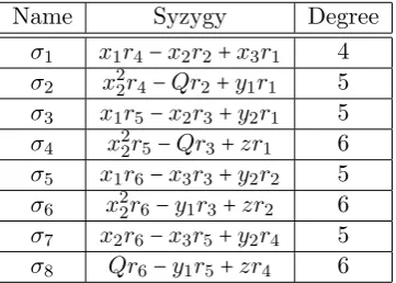
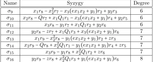
σ1∶= −x₁r₃+x₂r₂−y₁r₁ σ₁∶= −x₁r₃+x₂r₂−y₁r₁ σ2∶= −x₂r₃+x₃r₂−y₂r₁ σ₂∶= −x₂r₃+x₃r₂−y₂r₁

σ3∶= x₁r₅−x₂r₄+y₁r₂+x2₂x₃r₁ σ₆∶= x₁r₆−x₂r₅+y₂r₂+x₂x2₃r₁

σ4∶= x₂r₅−x₃r₄+y₁r₃+x3₁r₁ σ₇∶= x₂r₆−x₃r₅+y₂r₃+x2₁x₂r₁ σ5∶= y₁r₅−y₂r₄−x2₂x₃r₃+x3₁r₂ σ₈∶= y₁r₆−y₂r₅−x₂x2₃r₃+x2₁x₂r₂

(2.49) The best way to check that these eightσi generate the module of syzygies is

by using a computer algebra program (the relevant Magma code is in the appendix A.0 of this thesis).

Although these matrices certainly carry with the syzygies of the bicanonical ring, it turns out that deforming them to get one of the rings of the other 2 families is rather delicate. The procedure serves as a guide for the more complicated defor-mation calculations that we need to perform on the halfcanonical rings on curves and their extensions.

Both M1 and M2 have a zero of degree zero in their (1,2) entry, this

sug-gests to replace it by an affine parametert∈k so the fifth diagonal Pfaffian allows

us to express either y1 or y2 in terms of the degree 1 variables. One hopes that,

(40)

Pfaffians of both matrices simultaneously if we decide to deform one of the degree zero entries. Fortunately, the presentation has been purposely constructed so we can find a flat family deforming a bicanonical ring into a ring corresponding to an arithmetic genus 2 curve polarized by a degree 4 divisor defining a map onto a plane quartic with a cusp:

Lett∈k. I choose M₁ to decrease the codimension of the ring, thus I must

truncate M2 eliminating its first row and column. I will make also adjustments to

the rest of the entries so fort≠0 I get a ring isomorphic tok[x₁, x₂, x₃, y]/I₁whereI₁

is an ideal generated by the 2×2 minors of a matrix of the formA₁of equation(2.46).

Consider M1(t) ∶= ⎛ ⎜ ⎜ ⎜ ⎜ ⎜ ⎝

t x1 x2 y1

x2 x3 y2

y1 −x2₂x₃−t(x3₂+x₂y₁) −x3₁+t(x₁x2₃−x₃y₁)

⎞ ⎟ ⎟ ⎟ ⎟ ⎟ ⎠

and _M̃

2(t) ∶= ⎛ ⎜ ⎜ ⎜ ⎝

x2 x3 y2

y2 −x2x23−t(x22x3)

−x2₁x₂−tx2₁x₃ ⎞ ⎟ ⎟ ⎟ ⎠ .

Obviously the 4×4 Pfaffians of these matrices generate a bicanonical ideal when t=0. I claim that for t≠0 they generate the same ideal asy₁−x₁x₃+x2₂ together

with the 2×2 minors of ⎛

⎝

y2 x22+x2x3 −x1 x21−x

2

3 y2 x2

⎞

⎠. I also claim this defines a flat family