An empirical planetesimal belt radius–stellar luminosity relation

(1)

warwick.ac.uk/lib-publications

Original citation:

Matrà, L., Marino, S., Kennedy, Grant M., Wyatt, M. C., Öberg, K. I. and Wilner, D. J. (2018)

An empirical planetesimal belt radius–stellar luminosity relation. The Astrophysical Journal,

859 (1). 72. doi:10.3847/1538-4357/aabcc4

Permanent WRAP URL:

http://wrap.warwick.ac.uk/102997

Copyright and reuse:

The Warwick Research Archive Portal (WRAP) makes this work by researchers of the

University of Warwick available open access under the following conditions. Copyright ©

and all moral rights to the version of the paper presented here belong to the individual

author(s) and/or other copyright owners. To the extent reasonable and practicable the

material made available in WRAP has been checked for eligibility before being made

available.

Copies of full items can be used for personal research or study, educational, or not-for-profit

purposes without prior permission or charge. Provided that the authors, title and full

bibliographic details are credited, a hyperlink and/or URL is given for the original metadata

page and the content is not changed in any way.

Publisher’s statement:

Reproduced by permission of the AAS.

Published version:

http://dx.doi.org/10.3847/1538-4357/aabcc4

A note on versions:

The version presented here may differ from the published version or, version of record, if

you wish to cite this item you are advised to consult the publisher’s version. Please see the

‘permanent WRAP URL’ above for details on accessing the published version and note that

access may require a subscription.

(2)

AN EMPIRICAL PLANETESIMAL BELT RADIUS - STELLAR LUMINOSITY RELATION

L. Matr`a,1,∗ S. Marino,2 G. M. Kennedy,3M. C. Wyatt,2 K. I. ¨Oberg,1and D. J. Wilner1

1_{Harvard-Smithsonian Center for Astrophysics, 60 Garden Street, Cambridge, MA 02138, USA}

2_{Institute of Astronomy, University of Cambridge, Madingley Road, Cambridge CB3 0HA, UK}

3_{Department of Physics, University of Warwick, Gibbet Hill Road, Coventry, CV4 7AL, UK}

(Received 2017 December 22; Revised 2018 March 09; Accepted 2018 March 31)

ABSTRACT

Resolved observations of millimetre-sized dust, tracing larger planetesimals, have pinpointed the location of 26 Edgeworth-Kuiper belt analogs. We report that a belt’s distanceRto its host star correlates with the star’s luminosity L?, following R ∝ L0?.19 with a low intrinsic scatter of ∼17%. Remarkably, our Edgeworth-Kuiper belt in the Solar

System and the two CO snow lines imaged in protoplanetary disks lie close to this R-L? relation, suggestive of an

intrinsic relationship between protoplanetary disk structures and belt locations. To test the effect of bias on the relation, we use a Monte Carlo approach and simulate uncorrelated model populations of belts. We find that observational bias could produce the slope and intercept of theR-L? relation, but is unable to reproduce its low scatter. We then repeat

the simulation taking into account the collisional evolution of belts, following the steady state model that fits the belt population as observed through infrared excesses. This significantly improves the fit by lowering the scatter of the simulated R-L? relation; however, this scatter remains only marginally consistent with the one observed. The

inability of observational bias and collisional evolution alone to reproduce the tight relationship between belt radius and stellar luminosity could indicate that planetesimal belts form at preferential locations within protoplanetary disks. The similar trend for CO snow line locations would then indicate that the formation of planetesimals and/or planets in the outer regions of planetary systems is linked to the volatility of their building blocks, as postulated by planet formation models.

Keywords:submillimetre: planetary systems – planetary systems – circumstellar matter – Kuiper belt: general – protoplanetary disks – stars: individual (HD 377, HD 8907, 49 Ceti,τ Ceti, HD 15115, HD 21997, Eridani,β Pictoris, HD 61005, HD 95086, HD 104860, HD 107146,η Corvi, HD 111520, 61 Vir, HD 121617, HD 131488, HD 131835, HD 138813, HD 145560, HD 146181, HD 146897, HD 181327, AU Microscopii, Fomalhaut A, HR 8799).

[email protected]

∗_{Submillimeter Array (SMA) Fellow}

(3)

1. INTRODUCTION

The ubiquity of gas-poor, optically thin dust disks, known asdebris disks, around main sequence stars tells us that belts of planetesimals are a likely outcome of the planet formation process (for a review, seeMatthews et al. 2014). Planetesimal belts may form in the younger, dust- and gas-rich environments of protoplanetary disks, where the bulk of planet formation is thought to take place, but may also be produced after gas dispersal as a by-product of terrestrial planet formation. Formation in protoplanetary disks is likely for extrasolar Kuiper belts in the outer regions of planetary systems, as indicated by the increasing number of detections of large amounts of gas in young (_.few tens of Myr), cold (_&10 au) debris disks (e.g.Greaves et al. 2016;Lieman-Sifry et al. 2016;

Mo´or et al. 2017). However, why and how planetesimal belts arise remains largely unknown, and observations of individual systems provide few constraints on this pro-cess (Wyatt et al. 2015).

One aspect of planetesimal belts that can be linked to their formation mechanism is their location, which should remain unchanged over long timescales once the planets have formed and settled to a stable configura-tion. This is particularly true given that the observed evolution of belt masses (at least around A stars) ar-gues for the majority of the belt population being narrow rings (Kennedy & Wyatt 2010). The presence of a plan-etesimal belt in a planetary system tells us that, at that location, grain growth must have been efficient enough to form planetesimals, although some mechanism must have also been in place to either prevent further growth into planets, or to remove planets from these regions fast enough to produce a second generation of planetesimals before the gas-rich protoplanetary disk dissipated. Can these conditions arise anywhere in a planetary system? Or are there specific locations where these mechanisms giving rise to planetesimal belts preferentially act?

Current planet and planetesimal formation theories predict that planet and/or planetesimal formation ef-ficiency is a function of distance to the central star. In the core accretion scenario, this naturally arises from timescale and temperature arguments (e.g. Lis-sauer 1987;Lewis 1974). We focus on distances of tens of au, where most known planetesimal belts are observed. Growth timescales increase further away from the star, so for a given protoplanetary disk lifetime, planets may only have enough time to form out to a certain dis-tance, leaving a planetesimal belt beyond. At the same time, temperatures decrease with distance to the central star, creating several compositional transitions, orsnow lines, beyond which gas species of increasing volatility can freeze out onto solid grains (e.g. Cuzzi & Zahnle

2004). This can affect growth in different ways, for ex-ample through the sticking and fragmentation efficiency of particles (e.g.Wada et al. 2009;Okuzumi et al. 2016), but also by creating pressure gradients in the gas af-fecting particle concentrations (e.g.Stevenson & Lunine 1988). In general, theory would therefore suggest that the presence of a planetesimal belt, be it caused by failed growth to planets or enhanced planetesimal formation, should relate to distance to the central star. This moti-vates studies that observationally constrain the location of planetesimal belts as a population, and that test its dependence with host star properties - such as mass and luminosity - which directly affect the radial dependence of planet and/or planetesimal formation efficiency.

Such studies have so far been limited by the fact that, for the vast majority of belts, we only have unresolved IR multiband photometry constraining the dust tem-perature T of the small grains. This gives us a rough idea of a belt’s location under the assumption that the grains emit as blackbodies, giving us their blackbody ra-diusRBB. Several studies have analyzed the dependence

of dust temperature on host star properties (e.g. Chen et al. 2014; Jang-Condell et al. 2015), with Ballering et al. (2013) for example finding that the temperature of outer belts correlates with the temperature of the host star. However, it is well established that the small grains traced by the temperature of the spectral energy distribution are generally hotter than blackbody by an amount that is dependent on the grain properties and the size distribution; this means that RBB only truly

gives us a lower limit to a belt’s locationR (e.g.Booth et al. 2013).

Studies such as that ofBallering et al.(2017) alleviate this effect by accounting for the dust’s optical proper-ties, assuming all belts share the same composition, and finding that the radial location of warm, inner belts in-creases around stars with increasing masses, once again with a large scatter. In addition, Herschel marginally resolved a considerable number of cold dust disks (e.g.

(4)

Chiang 2006) and may therefore not directly trace the location of the parent planetesimals.

A solution to these issues is to resolve belts through millimetre wavelength interferometry, where the star is in most cases too faint to be detected, the resolution is sufficiently high to resolve even the smallest disks, and mm-sized grains are not subject to radiation forces, re-maining in the same low eccentricity orbits as the plan-etesimals they are created from (e.g. Wyatt 2006). We here present a first population study of planetesimal belt locations derived through millimeter wavelength in-terferometric observations. In §2 we introduce the full sample of interferometrically resolved planetesimal belts from the literature, showing that the distance of a belt from its host star (i.e. its radius) correlates with the star’s luminosity. In §3 we qualitatively and quantita-tively analyse the impact of observational bias, showing its importance in assessing the nature of correlations obtained from biased datasets. Having established the likely presence of an underlying correlation, in §4 we proceed to interpret the correlation in the context of both the collisional evolution and the formation loca-tion of planetesimal belts, and consider its potential im-plications for planetesimal and planet formation at large orbital separations. We conclude with a summary of our findings in§5.

2. RESULTS

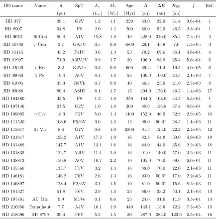
We collected all resolved Submillimeter Array (SMA) and Atacama Large Millimeter/submillimeter Array (ALMA) interferometric observations of planetesimal belts at millimetre/submillimetre wavelength published to date, to form a final sample of 26. Table1shows their belt and host star properties, as obtained from resolved observations in the literature and spectral energy distri-bution (SED) fitting (where the latter constrained the stellar luminosity, blackbody radius, and belt fractional luminosity, as described in Kennedy & Wyatt 2014). We note that, for the less well resolved objects in our literature sample, SED and visibility fitting were used simultaneously to constrain the disk’s surface density distribution (e.g.Steele et al. 2016).

We choose the belt location (radius) R to be repre-sented by either the average between the best-fit inner and outer belt radii (for models with a power law ra-dial surface density distribution and abrupt cut-offs), or by the best-fit centroid in the case of models with a Gaussian surface density dependence on radius. We con-servatively assume our uncertaintydRto be represented by half the best-fit radial width of the belt ∆Rfor cases where the width is well resolved, and by half the upper limit on ∆R for the three cases where the widths are

10

1

10

0

10

1

L

(

L

)

10

1

10

2

R

(A

U

[image:4.612.315.559.74.268.2]

)

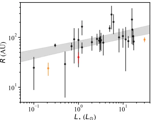
Figure 1.Observed planetesimal belt radii vs stellar lumi-nosities. The black bars represent the measured extent of debris belts in case belt widths are resolved, and an up-per limit to the extent in case they are unresolved (from Table 1). The shaded region represent the range of power laws with likelihood within±1σof the best-fit, including the intrinsic scatter as well as the uncertainty on the derived parameters. The orange error bars represent the observed lo-cation of the CO snow line in the two protoplanetary discs (TW Hydrae and HD 163296,Schwarz et al. 2016;Qi et al. 2013,2015) and the red error bar represents the radial ex-tent of the Kuiper belt (30-50 AU, Stern & Colwell 1997). We assume a main-sequence luminosity of 0.16 and 34 L

for TW Hydrae and HD 163296, respectively, based on their estimated stellar masses of 0.6−0.8 and 2.3M, respectively

(Webb et al. 1999;Natta et al. 2004).

unresolved (marked by the?symbol in Table1). As con-sidered later in§3.4, this choice of RanddRinevitably affects our analysis, but not our main conclusions. We determine the stellar luminosityL?as the integral of the

observed stellar intensity across all wavelengths. As shown in Fig. 1, we find a correlation between belt radii and the luminosity of their host star. The correlation is well represented by a power law model where the belt locations Ri (in au) are linked to their

host star luminosities L?,i (in L) through the form Ri = R1LL

α

?,i +i, where i represents the

intrin-sic scatter of the distribution, which we assume to fol-low a Gaussian distribution with standard deviation σintr=f∆RRi. Assuming this power law model, we take

an uninformative uniform prior on the free parameters R1L, α and f∆R, and a likelihood function described by Eq. 24 inKelly(2007), assuming Gaussian errors on radii and taking into account the intrinsic scatterf∆R.

(5)

[image:5.612.88.522.80.520.2]

Table 1.Properties of the sample of planetesimal belts resolved at mm wavelengths

HD name Name d SpT L? M? Age R ∆R RBB f Ref.

(pc) (L) (M) (Myr) (au) (au) (au)

HD 377 39.1 G2V 1.2 1.1 220 63.0 32.0 31.4 3.6e-04 1

HD 8907 34.8 F8 2.0 1.2 200 80.0 52.0 46.5 2.3e-04 1

HD 9672 49 Ceti 59.4 A1V 15.8 1.9 40 228.0 310.0 85.4 7.2e-04 2

HD 10700 τ Ceti 3.7 G8.5V 0.5 0.9 5800 29.1 45.8 7.0 1.3e-05 3

HD 15115 45.2 F4IV 3.6 1.3 23 78.2 69.6 55.1 4.6e-04 4

HD 21997 71.9 A3IV/V 9.9 1.7 30 106.0 88.0 65.4 5.6e-04 5

HD 22049 Eri 3.2 K2Vk: 0.3 0.8 600 69.4 11.4 19.5 4.0e-05 6

HD 39060 βPic 19.4 A6V 8.1 1.6 23 100.0 100.0 24.3 2.1e-03 7

HD 61005 35.3 G8Vk 0.7 0.9 40 66.4 23.6 21.0 2.3e-03 8

HD 95086 90.4 A8III 6.1 1.7 15 204.0 176.0 46.5 1.4e-03 17

HD 104860 45.5 F8 1.2 1.0 250 164.0 108.0 44.5 5.3e-04 1

HD 107146 27.5 G2V 1.0 1.0 200 88.6 126.8 37.8 8.6e-04 9

HD 109085 ηCrv 18.3 F2V 5.0 1.4 1400 152.0 46.0 52.9 2.9e-05 10

HD 111520 108.6 F5/6V 3.0 1.3 15 96.0 90.0? 58.5 1.1e-03 11

HD 115617 61 Vir 8.6 G7V 0.8 1.0 6300 91.5 123.0 22.2 2.4e-05 12

HD 121617 128.2 A1V 17.3 1.9 16 82.5 54.8 30.0 4.9e-03 18

HD 131488 147.7 A1V 13.1 1.8 16 84.0 44.0 35.6 2.2e-03 18

HD 131835 122.7 A2IV 11.4 2.0 16 91.0 140.0 57.0 2.2e-03 11

HD 138813 150.8 A0V 16.7 2.2 10 105.0 70.0 69.6 6.0e-04 11

HD 145560 133.7 F5V 3.2 1.4 16 88.0 70.0 22.0 2.1e-03 11

HD 146181 146.2 F6V 2.6 1.3 16 93.0 50.0? 17.0 2.2e-03 11

HD 146897 128.4 F2/3V 3.1 1.5 10 81.0 50.0? _15.6 _8.2e-03 ₁₁

HD 181327 51.8 F6V 2.9 1.3 23 86.0 23.2 50.1 2.1e-03 13

HD 197481 AU Mic 9.9 M1Ve 0.1 0.6 23 24.6 31.6 11.9 3.3e-04 14

HD 216956 Fomalhaut 7.7 A4V 16.1 1.9 440 143.1 13.6 72.2 7.5e-05 15

HD 218396 HR 8799 39.4 F0V 5.5 1.5 30 287.0 284.0 123.6 2.5e-04 16

Stellar luminositiesL?, fractional luminositiesf and blackbody radiiRBB obtained from spectral energy distribution (SED) fitting as described inKennedy & Wyatt(2014), except forEri, for which we use the fractional luminosity and blackbody

radius of the cold belt fromGreaves et al.(2014). Stellar massesM?are derived assuming stars have reached the

main-sequence, using tabulated values fromPecaut & Mamajek(2013), for all stars older than 20 Myr except low-mass AU Mic, which is still pre-main sequence and for which we adopt the mass value fromBoccaletti et al.(2015). For stars younger than 20 Myr, we use values fromPecaut et al.(2012) except for HD95086 (where we adopt the value fromMeshkat et al. 2013)

and HD138813 (Hern´andez et al. 2005). For HD121617 and HD131488 we found no literature value, which led us to adopt main-sequence values after verifying that the stars are close to reaching the main sequence (using tracks fromBaraffe et al. 2015). Ages are derived, where possible, from membership to Sco-Cen subregions (Pecaut & Mamajek 2016),βPic (Mamajek

& Bell 2014), Columba and Argus moving groups (Zuckerman et al. 2011). For HD377, HD8907, HD104860, HD107146, ages are fromSierchio et al.(2014) and references therein, forτ Ceti the age is fromMamajek & Hillenbrand(2008), forEri we adopt an average value in the range reported byJanson et al.(2015), forηCorvi the age is fromCasagrande et al.(2011), for

61 Vir fromValenti & Fischer(2005), and for Fomalhaut fromMamajek (2012). References for belt radius measurements: 1)

Steele et al.(2016): uniform surface density as a function of radius assumed. 2)Hughes et al.(2017): single power law model,

γ=−1.29. 3)MacGregor et al.(2016a): single power law model,γ=−0.3. 4)MacGregor et al.(2015): single power law model,

γ=−0.5. 5)Mo´or et al.(2013): single power law model,γ=−2.4. 6)Booth et al.(2017): Gaussian model. 7)Dent et al.

(2014): deprojected non-parametric dust distribution. 8)Olofsson et al.(2016): double power law model, ∆Rmeasured as full width at half maximum (FWHM). 9)Ricci et al.(2015), single power law model,γ= 0.74. 10)Marino et al.(2017b), Gaussian model. 11)Lieman-Sifry et al.(2016), single power law model withγ=−1.0 assumed (∆Rvalues marked by? were reported

as upper limits). 13)Marino et al.(2017a), single power law model,γ= 0.1. 13)Marino et al.(2016), Gaussian model. 14)

MacGregor et al.(2013), single power law model,γ= 2.3. 15)MacGregor et al.(2017), eccentric ring model. 16)Booth et al.

(6)

[image:6.612.52.286.56.293.2]

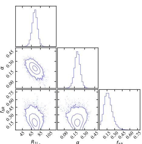
Figure 2.Marginalised posterior probability distributions of the power law parameters (slopeα, interceptR1L, and frac-tional intrinsic scatterf∆R)fitted to our observed data points

(Fig.1). These were sampled through MCMC methods as de-scribed in the main text. 1D histograms represent probability distributions of each parameter marginalised over the other two, whereas contour maps represent 2D probability distri-butions of different pairs of parameters, marginalised over the third. Contours represent the central [68.3, 95.5, 99.73] % of the distributions. Note that this fit does not take into account observational selection effects in [R, L?] space.

Monte Carlo (MCMC) approach. We implement the lat-ter through the_emceepackage (Foreman-Mackey et al. 2013) and using the affine-invariant sampler of Good-man & Weare (2010). Taking the 50+34₋₃₄ percentiles of the posterior distributions for our parameters (shown in Fig.2), we can set 1σ constraints onR1L = 73

+6

−6 au,

α= 0.19+0₋₀._.04₀₄ andf∆R= 0.17+0−0..0807.

3. BIAS ANALYSIS

While the tight constraints on the power law param-eters are indicative of a significant correlation, we need to consider whether our sample has been selected in an unbiased way within the [R, L?] parameter space

consid-ered here, which we will show not to be the case. In this Section, we therefore aim to verify and quantify whether selection effects applied to an uncorrelated population could have led to the observedR−L? relation.

3.1. Selection criteria

Three selection criteria determine whether a belt will appear on our [R, L?] plot: 1) detection of excess flux

due to dust at infrared (IR) wavelengths, the discovery method for planetesimal belts; 2) detection of the same

excess flux at millimeter wavelengths, and 3) resolvabil-ity of the belt with currently available mm-wavelength interferometric facilities. We here describe our treatment of these effects.

3.1.1. Infrared detectability

For IR excess detection, we require a belt to be brighter than 3 times the typical sensitivity of Spitzer

MIPS surveys (e.g. Su et al. 2006) at 24 µm (taken as the largest between 0.3mJy and 2% of the star’s 24 µm flux) and 70 µm (5mJy and 5%). If the belt is not detectable by Spitzer, we check whether it would have been selected and detected by the Herschel DEBRIS (e.g.Phillips et al. 2010) and DUNES (e.g.Eiroa et al. 2013) surveys at 100µm (1.5 mJy, 5%) and 160µm (3.5 mJy, 5%). When considering detectability, if a belt of ra-diusR is spatially resolved at any wavelength, we take into account that the sensitivity to a belt’s total flux density becomes different from the telescope’s surface brightness sensitivity. This is because the flux density of the belt is spread over Nres resolution elements, which

means that the uncertainty on the flux density becomes the telescope surface brightness sensitivity multiplied by √

Nres. We calculateNresas the number of resolution

el-ements covering the belt’s circumference, assuming the belt is viewed face-on and its width is unresolved. Al-though we take this effect into account, we find that it does not have a major effect on our results in the follow-ing Sections, as only a very small fraction of belts that are detectable are also faint and/or nearby and/or large enough to not pass this selection criterion.

3.1.2. Millimetre single-dish detectability

For a belt to have been targeted for resolved mil-limeter observations, we require it to have an 850 µm flux that would have been detectable by the JCMT through the SONS survey (sensitivity of∼1 mJy, Hol-land et al. 2017). Previous millimetre detection by single dish telescopes with similar sensitivities was the main selection criterion for most of the belts in our sample (18/26), the majority of which were detected by the SONS survey itself. The remaining 8 were detected at mm wavelengths for the first time and at the same time resolved by ALMA. Of these 8, six were resolved by

Lieman-Sifry et al. (2016), who selected them to have a bright fractional 70µm excess of at least 100, and two were resolved byMo´or et al.(2017), who selected them to be cold (Tdust <140 K), high-fractional luminosity

(f >5×10−4_{) belts around A stars. We use these}

(7)

In general, while we acknowledge that the adopted telescope sensitivities may be slightly better or worse for part of the observed population, we adopt them as a close approximation to the detection bias introduced, on average, for the majority of the population of belts in the Solar neighbourhood.

3.1.3. Millimetre interferometric resolvability

In order to allow a radius measurement, we also re-quire that a belt is resolvable over at least two resolu-tion elements for the highest resoluresolu-tion achievable with the ALMA interferometer at the wavelength that is most sensitive to dust emission with a millimetre slope typical of nearby planetesimal belts. This corresponds to 000.₀₂₈ at 870µm, and sets a hard lower limit on the radius of a belt that we are able to resolve.

In practice, another aspect to take into account when assessing a belt’s resolvability is whether the signal to noise ratio per resolution element (or in other words, the surface brightness sensitivity) is sufficient for accu-rate determination of a belt’s radius. In that context, we consider the fractional accuracy dR/R achieved when measuring the locationRof a narrow ring whose width is unresolved (as we are assuming here). The uncer-tainty dR can be estimated as ∼ FWHM/SNR where SNR is the signal to noise ratio achieved over one reso-lution element of size FWHM (in au) covering the ring width radially. Assuming the belt location is resolved (R > FWHM), that the ring is face-on, and employ-ing azimuthal averagemploy-ing to boost the SNR, we can write SNR∼Fν/(σres

√

Nres), where Fν is the total flux

den-sity of the belt (whereν∼345 GHz),σresis the

sensitiv-ity per resolution element of the instrument andNresis

the number of resolution elements across the ring’s cir-cumference (Nres= 2πR/FWHM). We therefore derive

thatdR/R∝pFWHM/R×σres/Fν.

We already required thatR >FWHM and that a belt is detectable by single-dish facilities at millimeter wave-lengths (F850µm>3 mJy). Noting that ALMA’s surface

brightness sensitivity is much better than this single-dish detectability threshold (σres F850µm), it follows

from the expression above that ALMA can accurately determine the radius of any belt that is detectable by single dish facilities.Therefore, the only requirement we adopt for resolvability is that a belt is large enough for its diameter to be resolved over at least two resolution elements with ALMA at 870µm (R >0.02800).

3.1.4. Optical thickness of small disks

Finally, we consider whether a belt has a small enough radius and/or high enough mass for its dust emission to become optically thick (see derivations in AppendixA). The optical depth to the line of sight τ can be simply

estimated for a face-on belt as the total cross sectional area in small grains divided by the on-sky area of the belt, resulting in the optical depth being proportional to the belt’s fractional luminosityf =Ldust/L? (as, for

example, in Jura 1991; Artymowicz & Clampin 1997). In particular, face-on belts with an assumed fractional width ∆R/R of 0.5 only become optically thick along the line of sight (τ > 1) if they have a fractional lu-minosity f > 2.5×10−1_{.We also consider an edge-on}

geometry, assuming a uniform density ring with ∆R/R of 0.5 and a scale heightH/Rof 0.1. In this case, their maximum optical depth along the line of sight reaches values > 1 for fractional luminosities f > 7.1×10−3. Since only few of the most massive belts that we con-sider in the following subsections (and only one of our observed belts) are affected, this effect is largely negli-gible for our population study.

3.2. Understanding the bias in[R, L?]space

We here test the hypothesis that these selection ef-fects alone applied to a population uncorrelated in [R, L?] space could reproduce our data. We use a Monte

Carlo approach, drawing a large population of model belts uniformly in log10([R, L?]) space and passing them

through our selection criteria (§3.1). However, assessing detectability and resolvability requires a model connect-ing a belt’s [R, L?] to its belt and host star’s flux as

ob-served from Earth at several wavelengths. We derive the host star’s flux at a given wavelength assuming black-body emission, and deriving all other stellar properties from L? assuming it has reached the main sequence,

interpolating tabulated values of Pecaut & Mamajek

(2013)1_.

To derive a disk’s flux from [R, L?] we use a simple,

narrow belt model as described inWyatt(2008), whose SED is described by a modified blackbody characterised by a temperature T, a fractional luminosity f, and a flux density (Fν) falling off as a power law with slope

(−2−β) at wavelengths larger then a givenλ0. We

re-mind the reader that a blackbody grain of temperature T derived from the SED would lie at a distance from the star equal to RBB, the so-called blackbody radius (see

Eq. 3 inWyatt 2008). In practice, small grains dominat-ing the SED are always hotter than blackbody, meandominat-ing that the true radius R of a belt as determined by re-solved mm-wavelength observations is always greater or equal toRBB. Throughout this work, we will use RBB

as an equivalent measure of temperature in order to cal-culate the belt flux. Thus, calculating the flux of a belt

1

(8)

[image:8.612.51.299.64.254.2]

Figure 3. Selection probability (%) per log10([R, L?]) bin

of a simulated population of belts drawn assuming a log-uniform distribution of fractional luminosities f between [10−7,10−2], a uniform distribution of R/RBB between [1.2,5.5], ofλ0 between [29.4,592.0]µm, and ofβ between [0.2,1.9]. Belt distances from Earth are drawn from an isotropic distribution (N(d)∝d2) out to 150 pc. White ver-tical bars represent our sample of belts currently resolved at millimeter wavelengths from Fig.1.

of known [R, L?] requires introducing extra free

param-etersRBB/R,f,λ0,β, as well asd, the distance to the

star from Earth.

This means that we have to make assumptions for these parameters that will impact the detectability of belts and hence affect the observational bias. We will test the effect of changing these assumptions in AppendixC, and here show results for our ‘fiducial’ model. For the latter, we assume a prior log-uniform distribution for f, a linearly uniform distribution for R/RBB, λ0 and

β, and log-uniform distributions for R and L? which

are not correlated with one another. The boundaries of the distributions of log10([R, L?]) are the same as the

plot boundaries in Fig.3. For the other parameters, we resort to empirical evidence from the extremes within our resolved belt sample to set our prior boundaries for f between [10−7_,₁₀−2_{], for}_R/R

BBbetween [1.2,5.5], for

λ0between [29.4,592.0]µm, and forβbetween [0.2,1.9].

Note that we will refer to this as a ‘static’ model, as (at least initially) we do not consider a belt’s evolution with time and its effect on these observables.

For each of theL? columns in Fig.3 we synthesize a

population of 4×105_{belts, 10}4 _{for each radius}_R

sam-pled in the vertical direction. Each of these belts is then assigned a set of parameters [f, R/RBB, λ0, β] drawn

from the assumed distributions described in the previous paragraph, and a distance from Earthddrawn assuming

a spherically isotropic distribution of stars (N(d)∝d2₎

out to a distance of 150pc, which is approximately the distance to the furthest star in our observed sample. Then, Fig.3 displays the fraction of the population of 104 _{belts simulated in each log}

10[R, L?] bin that would

pass our selection criteria derived in§3.1.

We find that the region where belt radii would have been selected has a triangular shape in [R, L?] space.

The upper and lower limits to selected radii are domi-nated, respectively, by the disk’s detectability at 70 and 850µm. This is because at any given stellar luminosity L?, for a fixed fractional luminosityf, belts increasingly

further from the star quickly become too cold for 70µm detection (due to the steep short-wavelength slope of the blackbody function). On the other hand, once again for a fixed fractional luminosityf, belts increasingly closer to the star more slowly become too warm for 850 µm detection (due to the shallower long-wavelength slope of the modified blackbody function). We remind the reader that the fact that belts can become too warm for sub-millimeter detection is because for a constant fractional luminosity, as assumed here, the dust mass is not con-stant but increases with radius (Mdust ∝ R2), hence

decreasing with temperature.

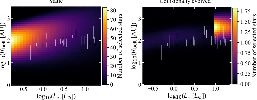
We highlight the fact that the colour map of Fig. 3

shows how the selection probability per bin varies in [R, L?] space; this significantly differs from the number

of selected stars per bin, which we present and discuss in AppendixB. Therefore, the colour map in Fig.3should not be compared with the density of observed points. Rather, we are interested in how vertical cuts in the colour map at a givenL? compare with the radius Rof

our observed belts.

3.3. Can theR−L? relation be explained by selection

bias alone?

The question we aim to answer is ‘Given our observed population of 26 stars, using our simple belt model with its assumptions and taking into account selection effects, what is the probability of having found ourR−L?

cor-relation if no corcor-relation was present?’. For each star in our sample of 26 resolved belts, we therefore take its known luminosity L? and distance d from Earth and

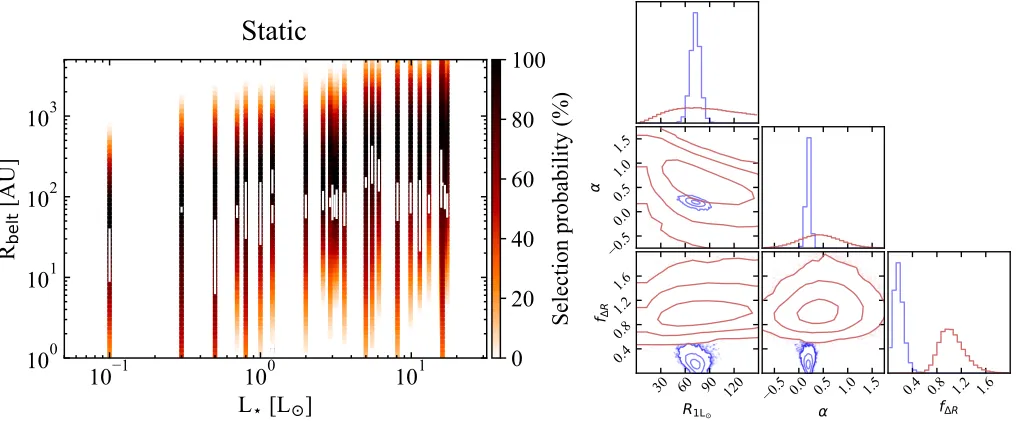
create a population of 106 belts, with the same fiducial model assumptions as employed in §3.2. For each star, we evaluate the fraction of belts that would be selected as a function of radius following our selection criteria. This yields a selection probability distribution of radii for each of our 26 stars (vertical color strips in Fig.4, left).

(9)

[image:9.612.54.562.65.276.2]

simu-Static

Figure 4.Results of Monte Carlo simulations of static model belt populations.Left:Vertical color strips represent the normalized selection probability of belts in log10(R) space for each of the stars in our sample, given their luminosityL?and distance from

Earth d. White vertical bars represent our sample of belts currently resolved at millimeter wavelengths from Fig. 1. Right: Marginalised probability distributions analogous to Fig.2, showing the results from fitting the data in blue). For comparison, red histograms and contours represent marginalised probabilities of randomly drawing a given set of parameters from an uncorrelated population of model belts, after accounting for observational selection effects

latedR−L?dependence through MCMC fitting, as done

for the observed data (§2). Using this approach requires assigning an uncertainty dR to the simulated radii R drawn for each L?. As this uncertainty affects the

de-rived intrinsic scatter of the relation (§2), given that we want to ensure fair comparison between the scatter of the simulated and observed populations, we assume each drawn radius at a given stellar luminosity to have the same fractional uncertaintydR/Ras that of the cor-responding observed belt.

We repeat this MCMC fitting for 105 _{simulations of}

the [R −L?] relation, and each time retrieve the set

of best-fit parametersR1L, αandf∆R. This allows us to obtain a 3D probability distribution of drawing the 3 observed power-law parameters from an uncorrelated [R, L?] population, which we show in Fig.4, right. These

simulated probability distributions (shown in red) can then be compared with the posterior probability distri-butions of the 3 parameters inferred from our observed data (blue, as derived in§2).

The probability distributions for our fiducial model in Fig.4 indicate that there is a modest probability of drawing a power law slope and intercept similar to the ones observed. Both the increasing upper envelope of IR detectability and the fact that more luminous stars in our sample tend to lie at larger distances d from Earth (increasing their smallest detectable radius) con-tribute to the result. On the other hand, we find that the marginalised probability (over all slopes and

inter-cepts) of finding an intrinsic scatterf∆R within±1σof

our observed value (0.17+0₋₀._.08₀₇) is below our capability to sample (< 10−5). In other words, none of our 105 simulated [R−L?] relations displays an intrinsic scatter

within±1σof our observed median value. This indicates that randomly drawing a highly correlated dataset such as ours from an uncorrelated population after taking bi-ases into account is very unlikely. This is mainly driven by the spread of our observed data points about the best-fit power law being much smaller than we would obtain from an underlying uncorrelated population.

Of course, this conclusion is dependent upon our as-sumptions for the set of parameters [f, R/RBB, λ0,

β] characterising the belt population. In Appendix C, we examine the effect that changing each of these pa-rameters has on our conclusion above. In summary, we find that while we cannot fully rule out that a specific combination of parameter assumptions may explain the observed R−L? relation, none of our reasonable sets

of assumptions (informed by our observed sample and previous IR population studies) can reproduce the ob-served population. In particular, the formal probability of drawing a relation consistent with ours from an uncor-related underlying population remains exceedingly low for all our tested assumptions, even for model popula-tions with R/RBB, λ0 and β fixed to a constant value

(10)

uncor-related [R, L?] population, which indicates that a true R−L?relation in the underlying population of belt radii

is likely necessary to explain our observed trend.

3.4. On the definition of the radius uncertaintydR

We note that our choice of uncertainties dR on the observed radii being equal to half the belt widths af-fects the derived parameters and their uncertainties. Nonetheless, we made this choice in light of two funda-mental issues. First, true uncertainties on the belt radius and width, which should be independently quantifiable, are not measured in a consistent way in different lit-erature works. The difficulty lies in the problem that most belts were fitted independently using a variety of parametrizations (see caption of Table 1), resulting in parameter uncertainties that do not easily translate to a radius uncertaintydR. Second, the choice of radius is itself dependent on which part of a belt is most rele-vant for its formation, which depends on which theory we are trying to test (see discussion in §4). Although our choice ofRas the ‘middle’ radius is somewhat arbi-trary, we deem it a more robust representation of where most of the dust is located than, for example, an inner or outer radius. The choice of radius of course also affects its own uncertainty, as well as our derived power law parameters. A major effort in consistently reanalyzing all archival datasets, which is beyond the scope of this paper, would be needed to enable us to change the defi-nition of radius and measure its associated uncertainty. Our main conclusion on the significance of the correla-tion stems from the fact that the scatter in the observed radii is small, and in particular smaller than would be expected from an underlying uncorrelated population. In other words, measured radii don’t fill the detectable [R, L?] space as well as expected from an uncorrelated

model population. This is despite the conservatively large uncertaintiesdRthat we assumed. Then, assuming smaller uncertainties would increase the inconsistency of the data with the model expectations, since observations would fill even less of the [R, L?] parameter space.

Investigating this issue more carefully, we can compare the intrinsic scatterf∆R of our measurement with that

expected from a randomly drawn, uncorrelated model belt population, as done in §3.3 above. This time, we test the effect of our assumption on dR by recalculat-ing probability distributions after fixrecalculat-ing dR/R=0.1 for both observed and simulated belt populations, for any stellar luminosity. These are shown as dotted lines in Fig. 8, top right, where the top row of Fig. 8 is oth-erwise equivalent to Fig. 4. As expected, this less con-servative choice for the uncertainties dR (i.e., smaller uncertainties) increases the intrinsic scatter needed to

fit the data. However, the same change applies to the model population, leaving the comparison between the two, and therefore our conclusion on the existence of an underlying R−L? relation, unaffected. Practically,

this is because the observed scatter of the data and the ‘observed’ scatter of the model population result from a combination of the intrinsic scatter and the assumed uncertainties dR. Then, changing the uncertainties in the same way for both the data and the model will only cause the derived intrinsic scatter to compensate in the same way for both, making the comparison largely in-dependent of the choice of uncertaintiesdR.

3.5. Quantifying the effect of selection bias on the uncertainty on derived power law parameters

Having concluded that an underlying correlation be-tween belt radii and their host star’s luminosity is likely necessary to explain the data, we here aim to quantify how selection bias affects the [R1L, α, f∆R] parameters derived through our power law fit to theR−L?relation

in§2, and in particular their uncertainties. We adopt the same MCMC fitting approach as in§2, but this time we modify the likelihood function of the power law parame-ters given the data to include selection effects, following the Bayesian method described in§5 ofKelly(2007). In summary, this acts by assigning higher probabilities to belts that are harder to detect, by weighting the contri-bution of the likelihood function from each belt radius by the inverse of the selection probability at that radius, as derived above in§3. This effectively counterbalances our selection effects and debiases our inference on the model parameters. Of course, our debiasing method remains dependent on the same assumptions for [f,R/RBB,λ0

andβ] as considered in the previous subsections. We here make the assumption of a belt population with log-uniform fractional luminosity and with fixed R/RBB, λ0 and β. Note that as demonstrated in

Ap-pendixC, fixing these values rather than drawing them from a distribution does not change the result signifi-cantly compared to the fiducial model. We findR1L= 66.8+7₋₁₁.7_.₈, α = 0.19₋+0₀._.05₀₆ and f∆R = 0.23+0−0..2710, where

these new debiased parameters are consistent with the biased ones. As expected, the uncertainties on the de-rived parameters increased because this debiased fitting takes into account that some undetected belts may lie in regions of low selection fraction. These debiased param-eters represent the properties of the underlying popula-tion after taking biases into account. Therefore, the fact that these parameters are inconsistent with the expecta-tion of an uncorrelated populaexpecta-tion (e.g.α= 0 and large f∆R), and that they are well constrained within their

(11)

Figure 5.Selection probability (%) per log10([R, L?]) bin of

a simulated population of belts whose dust mass has been evolved according to the model and best-fit parameters of

Wyatt et al.(2007) andSibthorpe et al.(2018). For a star of a given luminosity, an age is drawn from a uniform distribution up to the smallest between its main-sequence lifetime and the age of the universe. Belt distances from Earth are randomly drawn from an isotropic distribution (N(d) ∝ d2) out to 150 pc. White vertical bars represent our sample of belts currently resolved at millimeter wavelengths from Fig.1.

and the derived slope are robust against observational biases, at least for the fiducial population assumptions considered here.

4. DISCUSSION

Throughout§3, we analysed the effect of observational biases on the belt radius - stellar luminosity relation and demonstrated that it is likely that the observed rela-tion is caused by a true underlying correlarela-tion between the two parameters. We now analyse what the origin of this R−L? relation may be and whether it could

con-strain the belts’ formation location within protoplane-tary disks. In order to do that, we need to consider the effect of the collisional evolution over the belts’ lifetime.

4.1. Steady-state collisional evolution

A clear outcome of our bias analysis in §3 was that, regardless of the assumptions in our model, the sim-ulated populations after considering observational bias showed a scatter in radii that is much larger than ob-served. Under the log-uniform fractional luminosity as-sumption, the model prediction is that a large number of belts should have been detected and resolved at larger and smaller radii than the observed sample (as shown in Fig. 4, left). On the other hand, models with a log-uniform distribution of belt mass (see AppendixCand

Fig.8, bottom row) do a significantly better job of re-producing the lack of radii much larger than observed, but does a significantly worse job at reproducing the lack of belts with radii much smaller than observed. Overall, the distribution of dust masses (or fractional luminosi-ties) is the parameter that most significantly affects the scatter of the simulated belt populations.

What our static model of §3 did not consider is that belts are known to deplete and grind down over time, causing a decrease of their mass and fractional luminos-ity (e.g.Spangler et al. 2001). This decrease is faster for belts that have smaller radii and that have a higher mass stellar host, due to their planetesimals colliding at higher velocities. Therefore, for the same initial belt mass and radius at the beginning of collisional evolution, if we let belts around different stars evolve to the same system age, belts around low-luminosity stars and further from the star will be more massive than belts around higher luminosity stars and closer to the star. This implies that at a given system age, belts closer to the star and around more luminous stars will be less detectable. Conversely, we also need to consider that more luminous stars have a shorter main-sequence lifetime and are therefore on average observed at a younger age.

To test these effects expected from collisional evolu-tion, we once again resort to Monte Carlo methods and simulate the belt population predicted by the steady state collisional evolution model described in Wyatt

(2008). We assume that belts initiate collisional evolu-tion within protoplanetary disks, and therefore that they have been collisionally evolving for the entire lifetime of the star. The evolution of belt mass according to this model is almost flat up to an age roughly corresponding to the collision timescale of the largest bodies within the belt, after which the mass decreases with timet follow-ing 1/t.

This steady state collisional cascade model fits the ob-served evolution of IR excesses around both A and FGK stars (Wyatt et al. 2007; Kains et al. 2011; Sibthorpe et al. 2018), given some reasonable assumptions and other fitted parameters, which were found to differ for the two spectral type categories. We here adopt exactly the same assumptions and best-fit parameters to exam-ine the effect collisional evolution has on the observed belt population in [R, L?] space. In particular, for both

spectral type categories, the model assumes a universal belt fractional width of ∆R/R = 0.5, a grain density typical of silicates (ρ=2700 kg m−3_{), a proper}

eccentric-ity ofe= 0.05, an initial blackbody radius distribution of the belt population followingN(RBB)∝RγBB, and an

[image:11.612.51.299.60.258.2]

(12)

with a fitted centroidMmidand a standard deviation of

1.14 dex.

The distributions of both radii and initial masses are independent of stellar properties within each of the two spectral categories. For A (FGK) stars, fitted parame-ters with their best-fit values wereγ=−0.8 (γ=−1.7), Mmid = 10 M⊕ (Mmid = 2.1 M⊕), with the maximum planetesimal size Dc = 60 km (Dc = 450 km) and

dis-persal threshold planetesimal strengthQ∗_D= 150 J kg−1

(Q∗_D = 500 J kg−1) setting the time evolution. As no constraints are present to date for M stars, we assume the same parameters as for the FGK population. Fi-nally, since the model works by evolving belts located at their blackbody radii (which is consistent with the fact that the model was fitted to blackbody radii rather than true radii at IR wavelengths), we still need to make an assumption for the R/RBB distribution of the

pop-ulation. As in our fiducial model of §3, we assume a uniform distribution of R/RBB between the minimum

and maximum of our observed belt population.

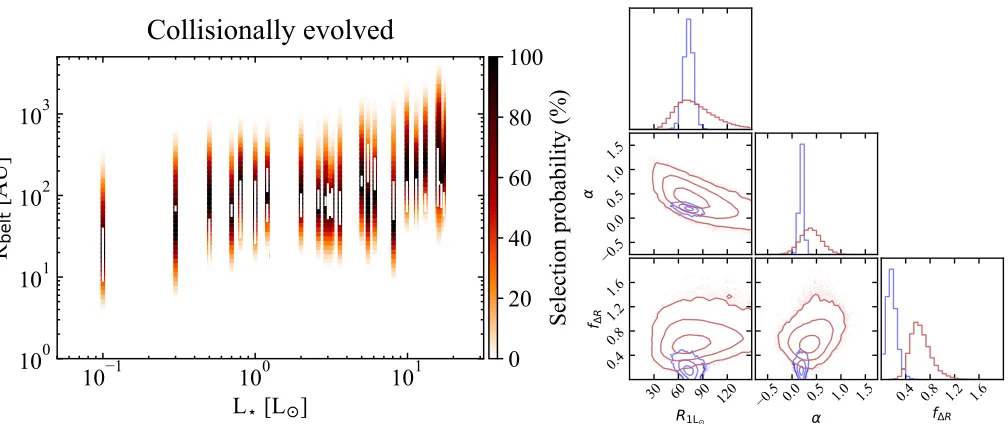
Informed by this collisional evolution model, we once again simulate a population of 106belts with the distri-bution of initial masses and radii that best fits the IR population. We evolve belts around each star to a ran-dom age drawn from a uniform distribution up to the lowest between the star’s main sequence lifetime and the age of the universe. In Fig.5we show the selection frac-tion per [R, L?] bin (analogously to Fig.3), assuming an

isotropic stellar population out to a distance of 150 pc. The main difference between Fig. 5 and Fig. 3 is that a new lower envelope of detectability appears at a larger radius than before, as belts that are closer to the star evolve faster and have their mass and hence flux dropping below detectability at any given age. If all belts were evolved to the same age, the dependence of this lower envelope on the stellar luminosity would be R∝L0.12

? (combining Eq. 6, 14, 15, and 16 fromWyatt

2008, and taking the approximation L? ∝ M?4).

How-ever, including the effect that less luminous stars are, on average, older than more luminous ones causes this lower envelope of detectability to be nearly flat. At the same time, this effect produces a steep dropoff in the number of detectable belts around stars of increasingly lower luminosity, as most of these belts have evolved for longer and hence depleted below detectability. The sharp discontinuity in the color map at high luminosi-ties is caused by the difference in the best-fit parameters fitted to the A and FGK star population at IR wave-lengths, which suggests that A stars evolve at a faster rate, but also start with more massive belts.

As mentioned for Fig.3in§3.2, we underline that the colour map in Fig. 5 does not consider the luminosity

functionN(L?) in the Solar neighbourhood and

there-fore should not be interpreted as the number of stars in [R, L?] space, which we show and discuss in Appendix

B. Once again, this is because we are not interested in reproducing the population density in [R, L?] space, but

the our observed R(L?) relation given our sample of

stars, with their luminosities, masses and ages.

We therefore proceed to quantify whether this steady state collisional evolution model for planetesimal belts can explain our observed trend as in §3.3, by quanti-fying the selection probability for each of the stars in our sample (see Fig. 6, left), given their L? and

dis-tance to Earth d. We evolve their belt mass to their observed age (choosing best-fit values reported in the literature, see Table 1), taking into account the distri-bution of belt radii from the collisional evolution model (N(RBB)∝R

γ

BB). We then sample each of these

prob-ability distributions 105 _{times and calculate the slope,}

intercept and intrinsic scatter of the simulatedR−L?

relations. The simulated probability distributions of the 3 power law parameters are shown in Fig.6(right, red), where they can once again be compared to the proba-bility distributions derived from the data (blue).

We find that the steady state collisional evolution ap-plied to a population of belt radii that is not correlated with their host star’s luminosity is likely to produce a R−L?relation with a slope and intercept close to those

shown by the data. Compared to our static belt model, the probability of drawing a dataset with an intrinsic scatter within±1σ of that observed (for any slope and intercept) increases significantly from the < 10−5

de-rived from Fig. 4 (right) to 2.6×10−3. This confirms the qualitative result of Fig.6 (left), showing that col-lisional evolution coupled to observational bias can re-produce the observedR−L? relation much better than

a static model (Fig.4, left). Despite the improvement, however, the probability of drawing an intrinsic scatter as low as that of the observed population remains quite low. If we formally consider the chance of drawing, at the same time, a slope, intercept and intrinsic scatter within ±1σof the observed values, the probability drops to an even lower value of 10−4_.

This indicates that one or more of the assumptions of the evolutionary model may not accurately describe the observed population. For example, the radii at which planetesimal belts form may not be well represented by a simple power law distribution as a function of black-body radius (N(RBB) ∝ R

γ

BB), as the comparison

(13)

[image:13.612.55.559.63.275.2]

Collisionally evolved

Figure 6. Results of Monte Carlo simulations of model belt populations, whose mass has been evolved according to the model and best-fit parameters ofWyatt et al.(2007) andSibthorpe et al.(2018). For both columns, lines and symbols have the same meaning as in Fig.4.

to both the population of resolved radii and IR excesses as a function of age is necessary to establish whether dif-ferent combinations of model parameters may quantita-tively reproduce the observed low scatter of theR−L?

relation.

4.2. A preferential formation location for planetesimal belts in protoplanetary disks?

An alternative explanation for the low scatter ob-served in the belt radii is that planetesimal belt loca-tions could be clustered at radii that depend on their host star’s luminosity. This would indicate a preferential location for planetesimal belt formation in protoplane-tary disks. This hypothesis is further supported by the location of the Edgeworth-Kuiper belt in our own Solar System (∼30-50 au,Stern & Colwell 1997) being close to the expectation from theR−L?relation seen in Fig. 1,

especially when considering that it does not suffer from the observational biases discussed in this work.

The question then arises as to what could cause plan-etesimal belts to form at a specific range of radii that correlate with the host star’s luminosity. As mentioned in§1, planetesimal belt formation requires grain growth to lead to the formation of planetesimals, but also a mechanism to either stop these planetesimals growing further to form planets, or to grow them into planets rapidly enough that several generations of planetesimals may be produced. Below, we consider possible scenarios that may fulfil these requirements for planetesimal belt formation.

4.2.1. Planetesimal formation and the CO snow line

It is now well established that formation of planetesi-mals fromµm-sized interstellar grains requires overcom-ing several growth barriers that are dictated by colli-sional physics and the interaction between solids and gas in protoplanetary disks. Collisional bouncing, fragmen-tation and erosion all act to slow the growth timescale of solids to the point they are lost to the star via radial drift before they can grow any further (for a review, see Birn-stiel et al. 2016, and references therein). A promising way to overcome these barriers is through particle over-densities leading to gravitational collapse, where such concentrations in the forms of disk substructure have re-cently started being discovered through high-resolution dust imaging of protoplanetary disks (e.g.van der Marel et al. 2013; Casassus et al. 2013; Marino et al. 2015;

ALMA Partnership et al. 2015; Andrews et al. 2016;

Isella et al. 2016;Loomis et al. 2017;Fedele et al. 2017). These overdensities can be caused by different physi-cal mechanisms; we direct the reader toJohansen et al.

(2015) for a review. We here focus on the CO snow line and its role in planetesimal formation; this is moti-vated by the fact that the radial location of the only two observationally-inferred CO snow lines (Qi et al. 2013,

2015;Schwarz et al. 2016) lies close to our [R−L?]

rela-tion (Fig.1). It has been theoretically demonstrated that snow lines can affect planetesimal formation in three ways. 1) Icy particles show increased sticking, favouring dust growth beyond the snow line location (e.g. Wada et al. 2009; Okuzumi et al. 2012). However, CO has a lower dipole moment compared to more polar ices such as H2O, which could actually lead to decreased sticking

(14)

2017). 2) Particles drifting inwards through the snow line lose their surface ice, causing a higher dust-to-gas ratio outside compared to just interior to the snow line (e.g. Stevenson & Lunine 1988; Cuzzi & Zahnle 2004). The evaporated gas may then diffuse beyond the snow line and freeze out onto incoming grains, leading to sig-nificantly enhanced growth at that location (Ros & Jo-hansen 2013), though further studies question the ef-fectiveness of the latter process at the CO snow line (Stammler et al. 2017). 3) Sintering of icy particles can lead to enhanced fragmentation and, conversely, reduce growth just beyond an snow line (e.g. Okuzumi et al. 2016).

On the observational side, the emergence and abun-dance of concentric rings in recent observations of pro-toplanetary disks may indicate a variation in dust opac-ities at the snow line location of different species. How-ever, this has been interpreted both ways as a sign of enhanced growth (Zhang et al. 2015) or fragmenta-tion (Okuzumi et al. 2016). Overall, it remains unclear whether the CO snow line would lead to an enhanced, reduced, or unchanged effectiveness of planetesimal for-mation.

The tentative association between planetesimal belt locations and CO snow lines reported here could there-fore indicate either of two scenarios. 1) Planetesimal for-mation is enhanced at the CO snow line location, and is followed by rapid planet formation and inward migra-tion. This mechanism could continue efficiently until the gas is dissipated, at which point the planetary system would be left with a belt of planetesimals that did not have time to further develop into planets just beyond the location of the CO snow line at the time of disk disper-sal. A similar scenario has been proposed to explain the composition of Uranus and Neptune in the Solar Sys-tem (Ali-Dib et al. 2014). 2) Planetesimal formation is

inefficient beyond the CO snow line location, leading to longer growth timescales which eventually allow plan-etesimals, but not planets, to form at these locations before the gas disk is dissipated.

Regardless of whether the R−L? relation for

plan-etesimal belts is related to planplan-etesimal formation at the CO snow line specifically, the similarity in slope be-tween planetesimal belt and the two observed CO snow line locations would indicate that volatility of solids in protoplanetary disks plays a crucial role in planetesimal and/or planet formation. In turn, this could imply a broad similarity in cometary compositions across plan-etary systems, explaining ice abundances being so far consistent between exocomets and Solar System comets (Matr`a et al. 2017a,b,2018).

4.2.2. Inefficient planet formation

Another approach to understanding the origin of plan-etesimal belts is to consider why planplan-etesimals did not go on to form planets, rather than why planetesimal themselves formed at specific locations in planetary sys-tems. Given the known presence of planetary or brown dwarf mass companions interior to planetesimal belts (e.g. Marois et al. 2008;Lagrange et al. 2009; Rameau et al. 2013; Macintosh et al. 2015; Milli et al. 2017), and even a potential correlation between the two ( Wy-att et al. 2012;Kennedy et al. 2015), a reasonable ques-tion to pose is whether planet formaques-tion simply did not have sufficient time to take place in the outer regions of planetary systems, where the mass budget is lower, and the orbital timescales are longer. If that were to be the case, given that both the solid masses increase (e.g.

Andrews et al. 2013) and the orbital periods shorten as function of stellar mass, it would make sense that plan-etesimal belts - which would be representative of the outer edge of planet formation - are observed to lie at larger radii around more massive (luminous) stars. Us-ing masses from Table1, ourR−L? relation translates

in a similarly correlatedR−M?relation. Neglecting the

effect of observational biases and collisional evolution, we find a power law dependence with slope αM? ∼1.0

(i.e.R∝MαM?

? ).

Then, a simplified way to understand whether planet formation timescales could set this relation is to con-sider the accretion timescale for a protoplanet to reach a massMpl and radiusRpl through core accretion from

a disk of planetesimals, and its dependence onM?.

Fol-lowing Kenyon & Bromley (2008), this timescale can be estimated as t ∝ 1

ΣΩ, where Σ is the local surface

density of planetesimals and Ω is the Keplerian angu-lar frequency, where Ω ∝ R−3/2_M1/2

? . We assume a

typical power-law planetesimal surface density profile (Σ(R) ∝ (M/Ry_out+2)Ry) with total mass in planetes-imals M and extending from the star out to radius Rout. We assume that the disk’s average surface

den-sity is constant (R2

out ∝ M, as found for dust in

pro-toplanetary disks, Tripathi et al. 2017), which implies (Σ∝M−0.5y_Ry_{). We can then connect the total mass in}

planetesimalsM to the mass of the central star, assum-ing this dependence to be the same as observed for the dust mass in protoplanetary disks (whereMdust∝M?x,

withx∼1.5−1.9,Pascucci et al. 2016).

Thus, if planetesimal accretion successfully produced planets out to a radius set by this accretion timescale,

we would expect this radius to scale asR∝M

0.5(1−xy) 1.5−y

? .

(15)

1977; Hayashi 1981), the expectation would be that R ∝ M0.54−0.64

? , which is shallower than the slope we

reported here (αM?∼1.0).

This simple calculation goes in the right direction to show that our result that planetesimal belt radii in-crease around stars of increasing mass qualitatively fol-lows the expectation from a planet formation timescale perspective, although it produces a slope slightly shal-lower than observed. Furthermore, the timescales would not be quick enough, as this core accretion model can-not produce Uranus and Neptune in situ within the life-time of the Solar Nebula (e.g. Goldreich et al. 2004). A likely solution to several problems with this simple planetesimal accretion model has more recently been found through the pebble accretion model, where the growth rate is significantly sped up by the accretion of inward-drifting pebbles (e.g.Lambrechts & Johansen 2012; Bitsch et al. 2015). Then, the timescale issue is overcome and several embryos can rapidly form in the outer regions of the Solar Nebula, and by extension in other planetary systems. In terms of the R−M?

rela-tion for planetesimal belts, pebble accrerela-tion would act to explain planet formation out to the inner edge of our observed relation in a shorter timescale. The pebble ac-cretion rate and consequent planet formation timescale is highly dependent on the assumed protoplanetary disk parameters, making detailed comparison difficult.

Given our main result that the scatter (rather than the slope or intercept) of resolved planetesimal belts is unlikely to be reproduced by current collisional evolu-tion models and observaevolu-tional bias, perhaps a more im-portant aspect to consider is how planet formation can reproduce such scatter. We speculate that this may be related to the range of timescales for planet formation in different planetary systems. If we let this timescale vary in the simple core accretion calculation above, we find R ∝ t1/(1.5−y)_{, where assuming} _y ₌ ₋₃_/_{2 as for}

the MMSN yields R ∝ t1/3. The ±1σ scatter in radii found across the R−L? relation (grey region in Fig.

1) implies thatR+1σ_/R−1σ_≈₁_._{5, which would imply a}

variation in planet formation timescales of ∼3.4. This would make sense if gas-rich protoplanetary disks pro-ducing detectable debris disks survived, for example, be-tween∼3-10 Myr, where these numbers are comparable to the observed decay in disk fraction in star-forming regions (e.g.Hern´andez et al. 2008).

Regardless of the details of the potential formation scenarios discussed here, confirming that there is a pref-erential formation location for planetesimal belts that is correlated with the host star’s mass and luminosity would be important to provide one of the first extraso-lar constraints to such planet formation models at extraso-large

orbital separations. While confirmation requires expan-sion of the observational sample and a more complete model effort in the multi-dimensional parameter space of planetesimal belt observables, explaining its origin re-quires planet formation models and simulations to pro-vide more specific predictions on the fate of planetesi-mals at large orbital separations, across a range of host star properties. At the same time, increasing the num-ber of resolved snow lines in young protoplanetary disks, particularly across a range of stellar hosts, will also em-pirically contribute to confirming the potential link pro-posed here.

5. CONCLUSIONS AND SUMMARY

In this work, we collected radius measurements from all 26 extrasolar planetesimal belts resolved at millime-tre wavelengths to date, and analysed their dependence on host star properties. We report the discovery of a sta-tistically significant correlation between belt radii and

host star luminosities, followingR= 73+6₋₆L0.19

+0.04

−0.04

? .

We simulate planetesimal belt populations to under-stand the effect of observational bias in [R−L?] space.

Given a static ring model, we show that it is unlikely that a population of belts with radii that are uncorre-lated with the host star’s luminosities can explain the observedR−L?relation through selection effects alone.

This is largely due to the observed population having a much lower scatter than the simulated one. We find the latter to remain true for several different sets of reasonable model assumptions, although we do not for-mally rule out that a specific combination of population model assumptions may explain the observed low scat-ter. Nonetheless, our tests indicates that an underlying R−L?relation is likely necessary to explain the observed

correlation. After repeating the fit to the observed popu-lation by taking into account observational bias through our fiducial model assumptions, we find the best-fit pa-rameters of the relation to be largely unchanged, with

R= 66.8+7₋₁₁.7_.₈L0.19

+0.05

−0.06

? .

We then consider whether steady state collisional evo-lution of a population of belts that are once again un-correlated in [R−L?] space, coupled to observational

bias, could explain the R−L? relation. We do so by

evolving the mass of simulated belt populations accord-ing to the models that fit the population of IR excesses (Wyatt et al. 2007; Sibthorpe et al. 2018). Including collisional evolution in the model population can read-ily explain the observed lack of small belts, particularly around stars of increasing luminosities. This brings the intrinsic scatter of the simulated population closer to the one observed, and better reproduces the observedR−L?

(16)

intrinsic scatter of the evolved simulated population is still higher and only marginally consistent with the one observed. This suggests that some of the collisional evo-lution model assumptions need to be refined; in partic-ular, the R−L? relation could indicate a preferential

formation location for planetesimal belts in protoplane-tary disks.

We briefly discuss how such a preferential formation location may be qualitatively explained in the context of current theories of planetesimal and planet formation. In particular, we focus on the CO snow line and its po-tential impact on the formation of planetesimals, show-ing that the location of the 2 observationally-determined CO snow lines in protoplanetary disks is close to the ex-pectation from our R−L? relation. The similar slope

between planetesimal belts and CO snow lines would suggest that volatility is a driver of planetesimal and/or planet formation.

At the same time, we consider why planetesimals did not grow further to form planets; we speculate that the inner edge of these belts may be set by the timescale of outermost planet formation, which would qualitatively explain the positive slope of theR−L? relation.

How-ever, we find that this slope, in a simplified core accre-tion scenario, should be flatter than observed. The low scatter observed, on the other hand, may be due to a narrow range in planet formation timescales, and is in line with the expectation from core accretion and the range of observed protoplanetary disk lifetimes.

Our work shows that in order to shed more light on the origin of theR−L?relation we need to expand the

sample of resolved planetesimal belts, enabling simulta-neous modelling of their masses and time evolution as well as radii distributions. This will be crucial in con-firming that there is a preferential formation location of planetesimal belts, a finding that can set important new constraints on models of planetesimal and planet formation in the outer regions of the Solar System and extrasolar planetary systems.

LM acknowledges support from the Smithsonian Insti-tution as a Submillimeter Array (SMA) Fellow. GMK is supported by the Royal Society as a Royal Society Uni-versity Research Fellow.