warwick.ac.uk/lib-publications
Manuscript version: Author’s Accepted ManuscriptThe version presented in WRAP is the author’s accepted manuscript and may differ from the published version or Version of Record.
Persistent WRAP URL:
http://wrap.warwick.ac.uk/104860
How to cite:
Please refer to published version for the most recent bibliographic citation information. If a published version is known of, the repository item page linked to above, will contain details on accessing it.
Copyright and reuse:
The Warwick Research Archive Portal (WRAP) makes this work by researchers of the University of Warwick available open access under the following conditions.
Copyright © and all moral rights to the version of the paper presented here belong to the individual author(s) and/or other copyright owners. To the extent reasonable and
practicable the material made available in WRAP has been checked for eligibility before being made available.
Copies of full items can be used for personal research or study, educational, or not-for-profit purposes without prior permission or charge. Provided that the authors, title and full
bibliographic details are credited, a hyperlink and/or URL is given for the original metadata page and the content is not changed in any way.
Publisher’s statement:
Please refer to the repository item page, publisher’s statement section, for further information.
MULTILATTICES
DEREK OLSON, XINGJIE LI, CHRISTOPH ORTNER, BRIAN VAN KOTEN
Abstract. We formulate the blended force-based quasicontinuum (BQCF) method for multilat-tices and develop rigorous error estimates in terms of the approximation parameters: atomistic region, blending region and continuum finite element mesh. Balancing the approximation parame-ters yields a convergent atomistic/continuum multiscale method for multilattices with point defects, including a rigorous convergence rate in terms of the computational cost. The analysis is illustrated with numerical results for a Stone–Wales defect in graphene.
1. Introduction
A full twenty years has passed since the original proposal of the quasicontinuum method [36] captivated the materials science community with the potential to model material phenomena spanning vastly different length scales. The quasicontinuum (QC) method was among the first of the so-called atomistic-to-continuum (AtC) coupling algorithms which sought to bridge the gap between length scales from the nano to macroscale. A remarkable number of these AtC methods have been proposed since (see e.g. [51, 31, 28] for a thorough discussion of many of these), and recently a mathematical framework has begun to emerge to analyze and compare several of these methods for defects in crystalline materials comprised of a Bravais lattice. Indeed, all three of the blended force-based quasicontinuum method (BQCF), blended energy-based quasicontinuum (BQCE), and blended ghost force correction (BGFC) methods have recently been analyzed in the context of a single defect in a two or three dimensional Bravais lattice [25, 41] as has the optimization-based AtC approach of [35]. Analyses in two and three dimensional Bravais lattices also exist for the AtC method of [26], but this has not yet been extended to allow for defects. Meanwhile, the methods [30, 46, 45] have been shown to be consistent (or free of ghost forces) for pair potential interactions only.
In the present work, we resolve the long-standing challenge to develop a rigorous numerical analysis for AtC methods in the context of multilattices, which allows for more than one atom to be present in the unit cell of the crystal. This description includes important materials such as hcp metals, diamond structures, and recently discovered 2D materials such as graphene and hexagonal boron nitride.
Concretely, we generalise the formulation and analysis of the blended force-based quasicontinuum (BQCF) method. Our main result is that, for a point defect in a homogeneous host crystal, the BQCF method for multilattices exhibits the same rate of convergence as in the Bravais lattice case. This is in sharp contrast with the blended energy-based quasicontinuum method for which a reduced convergence rate is expected in the multilattice setting [41].
The present work represents the first analysis that has been undertaken that remains valid for an AtC method which permits defects in a two or three dimensional multilattice. Even analyses of AtC
DO was supported by the NSF PIRE Grant OISE-0967140 and NSF RTG program DMS-1344962. XL was supported by the Simons Collaboration Grant with Award ID: 426935. CO was supported by ERC Starting Grant 335120.
methods for defect-free multilattices remain extremely sparse: the homogenized QC method [2, 1], for example, only allows for dead load external forces while the cascading Cauchy–Born method was rigorously analyzed only in one-dimensional multilattices for phase transforming materials [13]. As its name entails, the BQCF method is a force-based AtC method where a hybrid force operator is constructed instead of a hybrid energy functional [14, 47, 48, 26, 7, 5]. The primary advantage of force-based methods is that the forces can easily be defined in a way to avoid spurious interface effects (ghost forces); that is, the defect-free perfect crystal is a bona fide equilibrium configuration of the AtC force operator. The cost of defining the BQCF method and other force-based methods to be free of ghost forces is that these force fields are no longer conservative, which creates significant challenges in their numerical analysis [15, 27]. The blended force-based methods, originally studied in [23, 7, 5, 26], seek to overcome this problem by a smooth blending between atomistic and continuum forces over a region called the blending, overlap, or handshake region. Similar force-based blending methods have also been applied to coupling peridynamics with classical elasticity [43].
An alternative to the force-based paradigm is the energy-based paradigm where a global, hybrid energy is defined which is some combination of atomistic and continuum energies. This encom-passes the original quasicontinuum method and many other offshoots and ancestors [36, 52, 3, 16, 49, 12, 18, 8]. The peril of these methods is the aforementioned ghost forces, and it remains open to construct a general, ghost-force free, energy-based AtC method for Bravais lattices in two or three dimensions. As such we do not concern ourselves with an energy-based AtC method for multilattices; however, see [41, 44] for promising directions.
1.1. Outline. We begin in Section 2 by formulating an atomistic model for a multilattice material describing a single point defect embedded in an infinite homogeneous crystal. This is a canonical extension of the framework adopted for Bravais lattices in [35, 25, 24, 17, 41].
In Section 3 we then formulate the BQCF method for this model and state our main results: (1) existence of a solution to the multilattice BQCF method and (2) a sharp error estimate. We also convert this error estimate to an estimate in terms of the computational complexity of the BQCF method in Section 3.4 which in particular allows us to balance approximation parameters to obtain a formulation optimised for the error / cost ratio. We present a numerical verification of these rates by testing the method on a Stone–Wales defect in graphene. The complexity estimates obtained for the BQCF method for point defects in multilattices match those estimates in [25] for Bravais lattices.
Finally, Section 4 covers the technical details needed to prove our main result, Theorem 6. These technical details can be seen as generalizations of the results of Bravais lattices, and the primary new component is having to account for shifts between atoms in the same unit cell.
1.2. Notation. We introduce new notation throughout the paper required to carry out the anal-ysis. For the convenience of the reader, we have listed many of these in Appendix B. Here, we briefly establish several basic conventions we make throughout. We use d and n to denote the dimensions of the domain and range respectively, calligraphic fonts (e.g. L,M) to denote lattices, sans-serif fonts (e.g. F,G) for n×d matrices, the lower case Greek lettersα, β, γ, δ, ι, χ are used as subscripts denoting atomic species, and the lower case Greek letters ρ, τ, σ denote vectors (bond directions) between lattice sites.
The symbol | · | is used to denote the `2 norm of a single vector in
Derivatives of functions f : Rd → Rn are denoted by ∇f : Rd → Rd×n and higher order derivatives by ∇jf. Given F : X → Y where X and Y are Banach spaces, we denote Fr´echet or Gateaux derivatives by δjF, j indicating the order. We will most commonly interpret these derivatives as (multi-)linear forms and use them whenY =R, in which case we will then write the Gateaux derivatives as
hδF(x), yi, x, y ∈X
hδ2F(x)z, y
i, x, y, z ∈X and so on for higher order derivatives.
We reserve D for specific finite difference operators (defined in (2.3) and (2.4)), and use BR to denote the ball of radius R about the origin.
We use the modified Vinogradov notationx.ythroughout the manuscript to mean there exists a positive constant C such that x ≤ Cy. Where appropriate, we clarify what the constant C is allowed to depend on; in particular if there is any dependence on approximation parameters then it will always be made explicit.
2. Atomistic Model
2.1. Defect-free Multilattice. We consider an infinite Bravais lattice, or simply a lattice, L, defined by
L :=FZd, for someF∈Rd×d, det(F) = 1, and d ∈ {2,3},
where the requirement det(F) = 1 is purely a notational convenience. From a physical standpoint by taking symmetry into account, it can be shown that there are only 14 unique physical lattices in 3D and five in 2D (see e.g. [51]); however, we consider the lattice to merely be a mathematical framework. A multilattice is then obtained by associating a basis of S atoms to each lattice site, and this is also referred to as a crystal when the Bravais lattice is interpreted as one of the unique physical lattices.
For each site ξ ∈ L, these S atoms are located inside the unit cell of ξ at positions ξ+pref
α for pref
α ∈Rd and α= 0, . . . , S−1. The multilattice is then defined by
M:=
S−1
[
α=0
L+pref
α .
We call each L+pref
α a sublattice; here the addition “+” means a translation of the lattice L by the vector pref
α . Without loss of generality, we further assumepref0 = 0 (one atom is always located
at a lattice site). Furthermore, we make the distinction between a lattice site, which we use to refer to a site in the Bravais lattice,L, and an atom which is an element in the multilattice M.
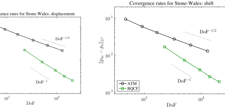
Two simple examples of multilattices are shown in Figure 1 including the 2D hexagonal lattice (e.g., graphene) for which
L=a0
√
3 √3/2 0 3/2
Z2, S = 2, p0 =
0 0
, p1 =a0
√ 3/2 1/2
, a0 =
√
2
33/4. (2.1)
(The a0 =
√
2
33/4 prefactor is due to the normalisation det(F) = 1.)
(a) 2D graphene: the dashed circles indicate the interaction neighbourhoods of the highlighted atoms.
[image:5.612.319.534.84.285.2](b) 3D rock salt: the interior cube represents a possible choice of unit cell.
Figure 1. Examples of multilattice structures.
currently be incorporated into the analysis. We further discuss the issues involved in this in our concluding discussion, Section 5. In the case of these out of plane displacements, we will useξ ∈R2
as both a vector in R2 and as the vector
ξ 0
∈R3. (We remark that though we will not consider dislocations, we could also consider n = 1 for an anti-plane screw dislocation model by fixing a second coordinate to be constant in this framework.)
The set of all sublattice deformations is denoted by y := (yα)S−α=01 and displacements by u := (uα)s−α=01. Equivalently we can describe the kinematics of a multilattice by a pair (Y,p) where Y :L →Rn is a deformation field and p
0, . . . , pS−1 :L → Rn are shift fields. The two descriptions
are related by
Y(ξ) = y0(ξ), pα(ξ) =yα(ξ)−y0(ξ); and yα(ξ) = Y(ξ) +pα(ξ),
and analogous expressions hold for displacements as well.
We now turn to a description of the energy. We will make the fundamental modeling assumption that the total potential energy of the system can be written as a sum of site potentials—that is,
ˆ
Ea
hom(y) :=
X
ξ∈L ˆ
V(Dy(ξ)), (2.2)
We use Dy(ξ) to denote the collection of finite differences (relative atom positions) needed to compute the energy at site ξ. More precisely, we specify a finite set of triples
R ⊂ L × {0,1, . . . , S−1} × {0,1, . . . , S −1} \ S−1
[
α=0
{(0αα)},
and use
D(ραβ)y(ξ) :=yβ(ξ+ρ)−yα(ξ) (2.3)
to denote the relative positions of speciesβ at site ξ+ρ and species α at site ξ. The collection of finite differences, or finite difference stencils, Dy, is then defined by
Dy(ξ) := D(ραβ)y(ξ)
(ραβ)∈R. (2.4)
In terms of (Y,p), this this notation becomes
D(ραβ)(Y,p) :=Y(ξ+ρ)−Y(ξ) +pβ(ξ+ρ)−pα(ξ) and D(Y,p) := D(ραβ)(Y,p))(ραβ)∈R.
For future reference we remark that we can write
D(ραβ)y=Dρyβ(ξ) +pβ(ξ)−pα(ξ),
where Dρf(ξ) :=f(ξ+ρ)−f(ξ). Moreover, we define the set of lattice vectors in R as
R1 :={ρ∈ L:∃(ραβ)∈ R}.
The site potential is then a function ˆV : (Rn)R
→R∪ {+∞}, where +∞allows for singularities in the potential (though we will later assume certain smoothness of the potential for convenience of the analysis).
Since the homogeneous reference configuration,yref, defined by
yrefα (ξ) :=ξ+pref
α , (2.5)
for constant pref
α ∈ Rn yields infinite energy, (due to an infinite sum over constant values of the site potential in the reference configuration), we thus will consider an energy difference functional defined on displacements from the reference state instead of (2.2). For a displacement u≡(U,p) from the reference stateyref let
V(Du(ξ)) = ˆV(D(yref +u)(ξ)),
and then the associated energy difference functional is defined by
Ea
hom(u) :=
X
ξ∈L
V(Du(ξ))−V(0). (2.6)
whereV(0) is a constant which will not affect minimization or force computations, so for simplicity, we assume without loss of generality thatV(0) = 0. In Theorem 2 below, we recall a result of [34] that characterizes for which displacements, u, Ea
A convenient notation for derivatives of V is the following: if (ραβ),(τ γδ) ∈ R and g = (g(ραβ))(ραβ)∈R ∈(Rn)R, we set
[V,(ραβ)(g)]i :=
∂V(g) ∂gi
(ραβ)
, i= 1, . . . , n,
V,(ραβ)(g) :=
∂V(g) ∂g(ραβ)
,
[V,(ραβ)(τ γδ)(g)]ij :=
∂2V(g)
∂g(jτ γδ)∂gi
(ραβ)
, i, j = 1, . . . , n,
V,(ραβ)(τ γδ)(g) :=
∂2V(g)
∂g(τ γδ)∂g(ραβ)
,
and note that this can be extended to derivatives of arbitrary order. Furthermore, we adopt the convention that if (ραβ)∈ R/ , then V,(ραβ)= 0.
The following standing assumptions on the interaction range and site potentials are made.
Assumption 1.
(V.1) The interaction range, R, satisfies
For each α∈ {0, . . . , S−1}, the set of vectors ρ such that (ραα)∈ R spans Rd,
and (0αβ)∈ R for all α6=β ∈ {0, . . . , S−1} .
(V.2) V is four times continuously differentiable with uniformly bounded derivatives and satisfies
V(0) = 0 (for simplicity of notation). Since V : (Rn)R → R, the statement that V has uniformly bounded derivatives means there exists M such that for any multi-index γ with
|γ| ≤4, |∂γV| ≤M.
We remark that (V.1) may always be met by enlarging the interaction range, R. On the other hand, (V.2) is made for simplicity of the analysis; it can be weakened to admit interatomic potentials with typical singularities under collisions of atoms, but this would introduce several additional technicalities in our analysis.
Next, we specify the function space over which Ehoma (u) is defined, which can be achieved in several equivalent ways. A convenient route is by first defining a continuous, piecewise linear interpolant of an atomistic displacement. Let Ta be a simplicial decomposition of L obtained as
in [25]: first let ˆT := conv{0, e1, e2} (where conv represents the convex hull of a set) be the unit
[image:7.612.180.436.112.242.2]triangle in 2D and ˆT1, . . . ,Tˆ6 six congruent tetrahedra in 3D that subdivide the unit cube (see
Figure 1 in [25] for an illustration in 3D) and then define
Ta =
(
{ξ+FT , ξˆ −FTˆ:ξ∈ L}, if d= 2,
{ξ+FTiˆ :ξ ∈ L, i= 1, . . . ,6}, if d= 3.
We will often refer to this as the atomistic triangulation or fully refined triangulation. As noted before, we may always enlarge the interaction range,R, so we may assume without loss of generality that
if conv{ξ, ξ+ρ} is an edge of Ta, then there exist α, β such that (ραβ)∈ R.
depending on which is notationally more convenient. Subsequently, we define the function space
U := u= (uα)S−α=01 :uα :L → Rn,kuka <∞ , where
kuk2a := S−1
X
α=0
k∇Iuαk2
L2(
Rd)+
X
α6=β
kIuα−Iuβk2
L2(
Rd).
Clearly, k · ka is not a norm on U since kuka = 0 only implies that each uα(ξ) is a constant
independent of α. However, k · ka is a semi-norm on U and hence a true norm on the quotient
space
U :=U/Rn:={(uα+C)S−α=01 :C∈R
n
} : u ∈ U .
Since the atomistic energy is invariant with respect to addition by constants, it is exactly this quotient space which we utilize as our function space. We also note that u and (U,p) are two equivalent descriptions for the displacements, and an equivalent norm on this space which will be convenient in terms of the (U,p) description is
k(U,p)ka :=k∇IUk2L2(
Rd)+
S−1
X
α=1
kIpαk2
L2(
Rd).
A dense subspace of U that we will use as a test function space is U0 where
U0 := {u∈ U : supp(∇Iu0), and supp(Iuα−Iu0) are compact},
U0 := U0/Rn.
As proven in [34], this test space is dense in U.
Lemma 1. [34, Lemma A.1] The quotient space U0 is dense in U.
2.2. Point Defect. We now introduce a framework to embed a point defect in a homogeneous multilattice. This problem has been heavily used in analyzing and comparing different AtC meth-ods for simple lattices in [35, 25, 28, 41] as it allows for a range of non-trivial benchmark problems and serves as a first step in analyzing more complicated scenarios such as interacting defects [21]. Point defects can be thought of as zero-dimensional defects representing a change to a single site in the lattice. Common examples include vacancies, interstitials, substitutions, and in graphene, the Stone–Wales defect which we use for our numerical verification.
Our first task is to define an analog ofEhoma for point defects, which is well-defined on the function space U. We accomplish this through a site-dependent site potential, Vξ, which must take into account the defective structure of the lattice near the defect core, which we assume to be at or near the origin. We then write the atomistic potential energy as
Ea
(u) :=X ξ∈L
Vξ(Du(ξ)). (2.7)
As in Assumption 1, we require certain smoothness of the site-dependent site potential in addi-tion to homogeneity outside of a defect core.
Assumption 2.
(V.3) There exists Rdef >0 such that Vξ ≡V for all |ξ| ≥Rdef.
We now recall from [34, Theorem 2.2] that Ea and Ehoma are well-defined on U; the main idea of the proof is that both are defined on displacements having compact support, and by density ofU0
in U, they may be uniquely extended by continuity to all of U.
Theorem 2. [34, Lemma 3.3] Assume the reference configuration yref with yref
α (ξ) = ξ+prefα is
an equilibrium configuration of the defect free energy meaning that
X
ξ∈L X
(ραβ)∈R ˆ
V,(ραβ)(Dyref(ξ))·Dv(ξ) = 0, ∀v ∈U0. (2.8)
Then Ea
hom(u) and Ea(u) may be uniquely extended to continuous functions on U which are C3 (three times continuously differentiable) on U.
Remark 1. The condition (2.8) that the reference configuration be an equilibrium is equivalent to requiring the shifts are equilibrated within each cell. See [34, Lemma 9] for details. Such reference configurations are thus straightforward to generate numerically.
Since we will eventually be working with a finite domain on which there is no difference between the original functionals and their extensions, we make no distinction between an energy and its continuous extension.
We are now able to pose the defect equilibration problem which we wish to approximate with the BQCF method, that is, to find u∞∈U such that
u∞∈arg min
u∈UE
a(u), (2.9)
where arg min represents the set of local minima of a functional.
While Assumptions 1 and 2 can be readily weakened in various ways, the next assumption concerning existence and stability of a defect configuration minimizing Ea is essential for our
analysis:
Assumption 3. (Strong Stability) There exists a solution, u∞, to (2.9) and a constant γa > 0 such that
hδ2
Ea
(u∞)v,vi ≥γakvk2a ∀v ∈U0.
Proving Assumption 3 turns out to be notoriously difficult; indeed the only result of this kind we are aware of is for a special case of a screw dislocation in a simple lattice [21, Remark 3.2] under anti-plane deformation. Nevertheless, we expect it to hold for virtually all realistic defects and realistic interatomic potentials. We also mention that it can be numerically checked a posteriori
once the defect configuration has been computed.
A useful consequence of Assumption 3 is the following regularity result, which is proven in [34] and extends the analogous simple lattice result [17]. These decay rates will be an essential com-ponent for converting the BQCF error estimates in terms of solution regularity that are presented in Section 3 into complexity estimates that are numerically verified in Section 3.4.
Theorem 3. [34, Theorem 2.5] For ρ=ρ1. . . ρk, the defect solution (U∞,p∞) satisfies
|DρU∞(ξ)|. (1 +|ξ|)1−d−k, for 1≤k≤3,
|Dρp∞α (ξ)|. (1 +|ξ|) −d−k
, for 0≤k ≤2, and allα = 0, . . . , S−1. (2.10)
The implied constant is allowed to depend on the interaction range through the maximum of |ρ|for
These decay rates will be an essential component for converting the BQCF error estimates in terms of solution regularity that are presented in Section 3 into complexity estimates that are numerically verified in Section 3.4.
Since we will compare discrete atomistic configurations with continuous finite element functions, it will be useful to reformulate Theorem 3 in terms of gradients of smooth interpolants, which we define in the next lemma (see [25] for further details and the proof).
Lemma 4. Letu:L →Rn, then there exists a unique functionIu˜ :
Rd→Rn withIu˜ ∈C2,1(Rd)
such that
(1) Iu˜ is multiquintic in ξ+F(0,1)d for each ξ ∈ L.
(2) Given any multiindex γ with |γ| ≤ 2, the interpolant satisfies ∂γIu(ξ) =˜ Dnn
γ u(ξ) where Dnn
γ are nearest-neighbor finite difference operators,
Dnni ,0u(ξ) := u(ξ),
Dnni ,1u(ξ) := 1
2(u(ξ+Fei)−u(ξ−Fei)) (ei is the ith standard basis vector), Dnni ,2u(ξ) := u(ξ+Fei)−2u(ξ) +u(ξ−Fei),
Dnn
γ u(ξ) := D
nn,|γ1|
1 · · ·D nn,|γd|
d u(ξ).
We will apply ˜I to both displacements and shifts using the notation ˜
I(U,p) = ( ˜IU,I˜p) = ( ˜U ,p˜).
Then, combining Theorem 3 and Lemma (4) yields the following result.
Theorem 5. The defect solution (U∞,p∞) satisfies
|∇jIU˜ ∞
(x)|. (1 +|x|)1−d−j, for j = 1,2,
|∇j ˜
p∞α(x)|. (1 +|x|) −d−j
, for j = 0,1,2, and all α= 0, . . . , S−1, (2.11)
where the implied constant is again allowed to depend on the interaction range, the site potential, and γa.
3. BQCF Method Formulation and Main Results
Any AtC approximation of the defect problem (2.9) must include the following ingredients: the atomistic and continuum domains, a coarsened finite element mesh in the continuum region, a specification of the continuum model, and finally and most importantly a mechanism for coupling the atomistic and continuum components.
We define the atomistic and continuum domains for the multilattice BQCF method by making similar choices as in the BQCF method for Bravais lattices [25]. We first give an intuitive descrip-tion of the domains involved, but will (re-)define them again below after introducing the blending function. Choose a computational domain Ω ⊂ Rd to be a (large) polygonal domain containing the origin (the defect). Fix a “defect core” region Ωcore such that, if Vξ 6≡ V, then ξ ∈ Ωcore.
Then take Ωa, the atomistic domain, to be a polygonal domain with Ωcore ⊂Ωa ⊂Ω, and set Ωc,
the continuum domain to be Ωc = Ω\Ωcore. In blending methods, the atomistic and continuum
domains overlap in a blending region Ωb = Ωc∩Ωa over which the atomistic and continuum forces
Next, we define a finite element mesh Th over Ω with nodes Nh. For now we only require that the finite element mesh is fully refined over Ωa, that is, if T ∩Ωa 6=∅, then T ∈ Th if and only if T ∈ Ta, but we will state further assumptions in Section 3.1.
The continuum model we adopt is the Cauchy–Born model [11, 9, 36], a nonlinear hyperelastic model, which is amenable to AtC couplings due to the definition of the strain energy density function in terms of the atomistic potential V,
WCB(G,p) := V
(Gρ+pβ−pα)(ραβ)∈R
for G∈Rn×d and p∈(Rn)S,
without resorting to any constitutive laws. We note that G here is the deformation gradient of lattice sites in a unit cell while p are the displacements of shift vectors; in contrast with typical continuum treatments of multilattices, we maintain the shift vectors as degrees of freedom in the Cauchy–Born model and do not minimize them out.
For W1,∞ displacement fields, U, and L∞ shift fields, p, this leads to a Cauchy–Born energy functional, formally (for now) defined by
Ec
(U,p) := Z
Rd
WCB(∇U(x),p(x))dx=
Z
Rd
V ∇(U,p)dx
where
∇(U,p) := ∇(ραβ)(U,p)
(ραβ)∈R := ∇ρU +pβ −pα
(ραβ)∈R is a continuum variant of the atomistic finite difference stencil
D(U,p)(x) = D(ραβ)(U,p)(x)
(ραβ)∈R := DρU(x) +pβ(x+ρ)−pα(x)
(ραβ)∈R.
The admissible finite element space we consider will beP1 finite elements for both the
displace-ments and the shifts subject to homogeneous boundary conditions. However, we will again consider equivalence classes of finite element functions by taking a quotient space. Thus, we define
Uh :=
u∈C0(Ω) :u|T ∈ P1(T), ∀T ∈ Th ,
Uh := Uh/Rn,
Uh,0 :=
u∈C0(Rd) :u|T ∈ P1(T), ∀T ∈ Th, u= 0 on Rd\Ω ,
Uh,0 := Uh,0/Rn,
Ph,0 :=
n
p= (p0, . . . , pS−1) :p0 = 0, and p1, . . . , pS−1 ∈ Uh,0
S−1o .
These spaces are endowed with the norm
k(U,p)k2ml :=k∇Uk2
L2(
Rd)+
S−1
X
α=0
kpαk2
L2(
Rd)=k∇Uk
2
L2(
Rd)+kpk
2
L2(
Rd),
where kpk2L2(
Rd) =
PS−1
α=0kpαk 2
L2(
Rd) is used for brevity. Along with the finite element space, we
also introduce the standard piecewise linear finite element interpolant,Ih, defined as usual through Ihu(ν) = u(ν) forν ∈ Nh.
The BQCF method is defined by blending forces on each degree of freedom, (ν, α) ∈ Nh ×
{0, . . . , S −1}, where the forces are defined by a weighted average of atomistic and continuum forces:
Fbqcf
ν,α (U,p) := (1−ϕ(ν))
∂Ea(U,p)
∂uα(ν) +ϕ(ν)
∂Ec(U,p)
where the blending function, ϕ, satisfies ϕ ∈ C2,1(Rd) with ϕ = 0 in Ωcore and ϕ= 1 in Rd\Ωa.
The BQCF method then seeks to solve Fν,αbqcf(U,p) = 0 for all ν /∈∂Ω. Equivalently, we can write the force balance equations in weak form using the variational operator
hFbqcf
(U,p),(W,r)i
:=X ν
X
α
Fbqcf
ν,α (U,p)·(W +rα) (ν)
=X ν
X
α
(1−ϕ(ν))∂E
a(U,p)
∂uα(ν) ·(W +rα) (ν) +ϕ(ν)
∂Ec(U,p)
∂uα(ν) ·(W +rα) (ν)
=hδEa(U,p),((1
−ϕ)W,(1−ϕ)r)i +hδEc
(U,p),(Ih(ϕW), Ih(ϕr))i, (3.2)
where the last equal sign comes from direct calculation. The BQCF approximation to the defect optimization problem (2.9) is then to find (U,p)∈Uh,0×Ph,0 such that
hFbqcf(U,p),(W,r)i= 0, ∀(W,r)∈U
h,0×Ph,0. (3.3)
The variational formulation is preferred for the analysis while the force-based formulation (from which the name BQCF is derived) is preferred for implementation. The pointwise formulation (3.1) was essentially how the original BQCF method was proposed for Bravais lattices [6], and this was analyzed in a finite-difference framework without defects for Bravais lattices in [26, 23]. The variational formulation (3.2) was introduced in [25] for Bravais lattices, and its subsequent analysis led to one of the first complete analyses of an AtC method capable of modeling defects.
3.1. Assumptions on the Approximation Parameters. We now summarise the precise tech-nical requirements on the approximation parameters, ϕ,Ω,Ωa,Ωb,Ωc,Th, which will be analogous to those in [25].
We begin by summarising basic assumptions on the blending function: (1) ϕ∈C2,1 and 0≤ϕ≤1
(2) If Vξ 6≡ V, then ϕ(ξ) = 0. This means that ϕ vanishes near any defect, hence the pure atomistic force is employed in those regions.
(3) There exists K > 0 such that ϕ(x) = 1 if |x| ≥K. That is, ϕ is identically one far away from the defect.
As the second step we specify the computational domain Ω and its corresponding partition Th. First, we shall require that supp(1−ϕ)⊂Ω always holds. To state the required properties forTh, we first precisely specify the sub-domains in terms of ϕ and Ω. Let
rcut := max{|ρ|: (ραβ)∈ R}
be an interaction cut-off radius, let rcell be the radius of the smallest ball circumscribing the unit
cell of L, and definerbuff := max{rcut, rcell}. Then we set
Ωa := supp(1−ϕ) +B4rbuff, Ωb := supp(∇ϕ) +B4rbuff,
Ωc:= supp(ϕ)∩Ω +B4rbuff, Ωcore:= Ω\Ωc.
The size and shape regularity of the various subdomains are parameterized in terms of inner and outer radii: for t∈ {a,c,b,core}, we set
rt:= sup
r {
r >0 :Br ⊂Ωt∪Ωcore}, Rt := inf
Rb
Ro
ri
∂Ω supp(∇ϕ)
[image:13.612.198.418.72.287.2]Ωcore (shaded area)
Figure 2. A diagram showing a selected number of domains and their inner and outer radii.
where we recall the notationBRto denote the ball of radiusRabout the origin. The corresponding outer and inner radii for the complete domain Ω are, respectively, denoted by Ro and ri:
ri := sup
r {
r >0 :Br⊂Ω}, Ro := inf
R {R >0 : Ω⊂BR}.
Finally, we define an overlapping exterior domain,
Ωext :=Rd\Bri/2,
which will be used to quantify the far-field error made by truncating to a finite computational domain.
For the sake of completeness, we now restate a crucial condition on the finite element mesh:
(4) The finite element mesh is fully refined over Ωa, that is, ifT ∩Ωa 6=∅, then T ∈ Th if and only ifT ∈ Ta.
To conclude this discussion we note that only the blending function ϕ and the finite element mesh Th are free approximation parameters, while the subdomains and corresponding radii are derived (in particular, Ω =S
Th). In our analysis we will require bounds on the “shape regularity” of ϕ,Th, and the domains defined above:
Assumption 4. In addition to (1)–(4) there exist constants CTh, Cϕ > 0, which shall be fixed throughout, such that
k∇jϕ
kL∞ ≤CϕR−j
a for j = 1,2,3, and max
T∈Th
σT
ρT ≤CTh,
where σT denotes the radius of the smallest ball circumscribing T and ρT the radius of the largest ball contained in T. Defining the mesh size function
h(x) := max T∈Th:
there exists s≥1 such that the mesh satisfies the growth condition
|h(x)| ≤CTh
|x| Ra
s
, |x| ≥Ra.
Moreover, there exists Co >0 and a positive integer λ such that
Ro ≤CoRλcore and
1
4Ra ≤Rcore≤ 3
4Ra. (3.4)
While Cϕ will feature heavily in our analysis, the parameter CTh will only enter implicitly in
the form of constants in interpolation error estimates. The condition 1
4Ra ≤ Rcore ≤ 3
4Ra greatly
simplifies the analysis. It is likely this could be weakened by an extremely refined analysis as can be done in one dimension [23], but the asymptotic estimates obtained would be unchanged with the exception of an improved prefactor so we do not pursue this. Moreover, though one can generate blending functions which satisfy these assumptions using splines, we point out that in practical implementations one can relax the regularity requirements on the blending functions, and this has provided no loss in performance in simulations carried out for lattices in [24].
3.2. Main Result. Our main result concerns the existence of a solution to (3.3) and an estimate on the error committed.
Theorem 6. Suppose that Assumptions 1, 2, and 3 are valid. Then there exists R∗
core such that, for any approximation parameters satisfying Assumption 4 as well as Rcore ≥R∗core, there exists a solution (Ubqcf,pbqcf)∈U
h,0×Ph,0 to the BQCF equations (3.3) that satisfies
k∇IU∞−∇Ubqcf
kL2(
Rd)+kIp
∞
−pbqcfkL2(
Rd) . γtr
kh∇2IU˜ ∞
kL2(Ω c)
+kh∇I˜p∞kL2(Ω
c)+k∇IU˜ ∞
kL2(Ω
ext)+kI˜p ∞
kL2(Ω ext)
,
(3.5)
where
γtr:=
( p
1 + log(Ro/Ra), if d= 2,
1, if d= 3.
The implied constant, as well as R∗
core, may depend on Cϕ and CTh, the interatomic potentials
V, Vξ, the maximum of |ρ| for ρ∈ R1, and the stability constant, γa.
Remark 2. The quantity γtr arises from a trace inequality that is needed when estimating
interpolants on the atomistic mesh in terms of interpolants on the continuum mesh, c.f. [Lemma
4.6][25].
Section 4 is devoted to proving Theorem 6, but before we embark on this, we first demonstrate how the error estimate can be combined with the regularity estimates of Theorem 5 to yield an optimised BQCF scheme with balanced approximation parameters. This is followed by a numerical test on a Stone–Wales defect in graphene, validating our theoretical convergence rates.
3.3. Optimal parameter choices. Once we restrict ourselves to a Cauchy–Born energy withP1
The choice of blending function is, in the case of the BQCF method, arbitrary as long as Assumption 4 is satisfied. There are many choices to make for the blending function which meet these requirements, see e.g. [29].
The finite element mesh and hence the choice of Ω may, however, be optimized. The key to choosing the finite element mesh and size of Ω lies in applying the decay results of Theorem 5 to our error estimate (3.5), [28, 24, 29]. In obtaining our optimized parameters, we do not provide rigorous proofs but instead use heuristic assumptions to arrive at approximate choices which can then be rigorously analyzed numerically. To start, we assume that the mesh size function h(x) is radial, i.e., h(x) ≡ h(|x|). Then, ignoring logarithmic factors in γtr and employing the estimate
|1 +r|−1 .r−1 for r≥1, the error estimate (3.5) can be further estimated by
k∇IU∞− ∇Ubqcf
k2
L2(
Rd)+kIp
∞
−pbqcfk2L2(
Rd)
. Z Rc
rcore
|h(r)|2r−3−d dr+
Z ∞
1/2ri r−1−d
dr
Next, we note that from the definitions of Ωc,Ω, and ri, we have ri =Rc+ 4rbuff so that we may
make the replacement ri ≈Rc. Denoting the number of degrees of freedom by DoF (nodes in the
continuum finite element mesh times the number of species in the multilattice), we can then carry out an optimization problem consisting of minimizing this error estimate subject to a fixed number of degrees of freedom, DoF. This problem is exactly the same as for the Bravais lattice and is
min h∈L2,R
c>0 Z Rc
rcore
|h(r)|2r−3−d dr+
Z ∞
1/2Rc r−1−d
dr.
This problem is solved in [32] where it is found that there are approximate minimisers of the
form h(r) = r/Ra
1+1+d/d2
. A simplified approximate solution can be obtained by first minimizing RRc
rcore|h(r)|
2r−3−ddr with respect to h where the same expression for h will result, but instead of
also minimizing with respect to Rc, one can simply note that the error then becomes
Z Rc
rcore
|h(r)|2r−3−d dr+
Z ∞
1/2Rc r−1−d
dr.r−d−2 core +R
−d
c . R
−d−2 a +R
−d
c . (3.6)
In order to balance the sources of error, one should take Rc =R 2/d+1
a . Finally, by simply writing
the number of degrees of freedom as the sum of those in the atomistic and continuum regions, it is possible to derive the result that #DoF≈Rd
a; further details can be found in [32, 33, 28, 25].
After making the estimation γtr ≤ (log DoF)1/2 [25] for d = 2, the main error estimate, (3.5),
currently written in terms of solution regularity, may now be replaced by an estimate of (3.6) in terms of computational cost since #DoF≈Rd
a:
k∇IU∞− ∇Ubqcfk2
L2(
Rd)+kIp
∞
−pbqcfk2L2(
Rd)
. (
(DoF)−1−2/dlog DoF, d= 2, (DoF)−1−2/d, d= 3,
(3.7)
which exactly matches the rate for the Bravais lattice case [25]. This is due to the fact that the limiting factor in both error estimates is the P1 finite element approximation.
Remark 3. In the Bravais lattice analysis [25], the expression of Rc in terms ofRa is incorrect
In that paper, a different mesh scaling is also used, but should the same mesh scaling be used, the error estimates in terms of the degrees of freedom would be identical up to a constant prefactor.
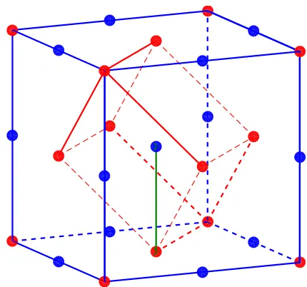
3.4. Numerical tests. In addition to providing a means to estimating the computational cost of the BQCF method, the estimate (3.7) is also convenient to verify numerically. We have carried this out for a Stone–Wales defect in graphene using both the BQCF method and a fully atomistic method.
For the latter we simply minimize the full atomistic energy over displacements that are non-zero only on the computational domain Ω (clamped boundary conditions). Using the methods discussed in Section 4, it is not difficult to show that the solution, (UDir,pDir), to this atomistic Galerkin
method exists and satisfies the error estimate
k∇IU∞− ∇UDirk
L2(
Rd)+kIp
∞
−pDirkL2(
Rd) . (DoF)
−1/2. (3.8)
We now set the model up for the Stone–Wales defect in graphene, recalling first the multilattice parameter values given in Section 2. We choose a Stillinger-Weber [50] type interatomic potential with a pair potential and bond angle potential component. The interaction range we consider is
R=(ρ100),(ρ200),(−ρ100),(−ρ200),(ρ1−ρ200),(ρ2−ρ100),
(001),(010),(−ρ201),(ρ210),(−ρ101),(ρ110),
(ρ111),(ρ211),(−ρ111),(−ρ211),(ρ1−ρ211),(ρ2−ρ111) ,
which is depicted in Figure 1. In this notation, the site potential is given by
ˆ
V(Dy(ξ)) = X
(ραβ)∈R 1
2φ(D(ραβ)y(ξ)) +ϑ(D(−ρ101)y(ξ), D(−ρ1−ρ201)y(ξ))
+ϑ(D(−ρ101)y(ξ), D(−ρ201)y(ξ)) +ϑ(D(−ρ1−ρ201)y(ξ), D(−ρ201)y(ξ))
+ϑ(D(ρ110)y(ξ), D(ρ1+ρ210)y(ξ)) +ϑ(D(ρ110)y(ξ), D(ρ210)y(ξ))
+ϑ(D(ρ1+ρ210)y(ξ), D(ρ210)y(ξ)),
where φ(r) = r−12−2r−6 is a pair potential term and
ϑ(r1, r2) =
r1·r2
|r1| |r2|
+ 1/22
is a three-body term that penalizes angles that differ from 23π.
The Stone–Wales defect shown in Figure 3 is obtained by rotating the bond between the two carbon atoms at the origin site by ninety degrees about the midpoint of this bond. One way of incorporating this defect into our framework is to define a reference configuration (Y0, p1) where
Y0(ξ) = Fξ for all ξ 6= 0 withF and p1 given by the graphene parameters in (2.1). At the origin,
we setY0(0) = Rot(0) and p1(0) = Rot(p1), where Rot represents the ninety degree rotation about
the midpoint of the segment conv{0, p1}. Then we set Vξ(D(U, p)(ξ)) = ˆV(D(Y0+U, p1+p)(ξ)).
We choose hexagonal domains for Ωcore,Ωa,Ω, etc., and use a blending function which
approxi-mately minimizes theL2 norm of∇2ϕon Ω
b [29]. We select the inner width, rcore, of the hexagon
Ωcore to be from the range Ra ={8,12,16,20,24} with κ = 1/2, and then the remaining domains
are chosen as scaled hexagons satisfying the requirements of Section 3 and Theorem 6 (see Figure 10 in [24] for a representative illustration of this domain decomposition for a Bravais lattice). Finally, our finite element mesh is graded radially with approximate mesh sizeh(r) = r
Ra 3/2
(a) A perfect graphene sheet. (b) An unrelaxed Stone–Wales defect.
Figure 3. Examples of a perfect graphene sheet and a Stone–Wales defect. The dotted lines in the right display indicate bonds that are broken during the rotation of the highlighted atoms.
conjugate gradient algorithm with line-search based on force-orthogonality only (in BQCF there is no energy functional for which descent can be imposed).
103 104
DoF
10-3 10-2 10-1
kr
Uac
!
r
Ua kL
2
Convergence rates for Stone-Wales: displacement
ATM BQCF
DoF!1
DoF!1=2
(a) Error in displacement field for Stone–Wales de-fect.
103 104
DoF 10-3
10-2 10-1
k
pac
!
pa kL
2
Covergence rates for Stone-Wales: shift
ATM BQCF
DoF!1
DoF!1=2
[image:18.612.143.524.76.258.2](b) Error in shift field for Stone–Wales defect.
Figure 4. BQCF error plotted against degrees of freedom. We have also plot-ted the “purely atomistic” error, denoplot-ted by ATM, which is the solution obtained by truncating the infinite dimensional atomistic problem to a finite domain using homogeneous Dirichlet boundary conditions.
4. Proofs
The remainder of this paper is devoted to proving our main result, Theorem 6. As in [25], the abstract framework for the proof is provided by the inverse function theorem [28, 37, 20], which we recall for reference and which is used to establish well-posedness of the nonlinear BQCF variational equation in Theorem 6.
Theorem 7 (Inverse Function Theorem [37, 20]). Let X and Y be Banach spaces with
f : X → Y, f ∈ C1(U) with U ⊂ X an open set containing x
0. Suppose that η > 0, σ > 0, and
L >0exist such that kf(x0)kY < η, δf(x0) is invertible with kδf(x0)−1kL(Y,X) < σ, B2ησ(x0)⊂U,
δf is Lipschitz continuous on B2ησ(x0) with Lipschitz constant L, and 2Lησ2 < 1. Then there exists a C1 inverse function g :Bη(y0)→B2ησ(x0) and thus an element x¯∈X such that f(¯x) = 0 and
kx0−x¯kX < 2ησ.
The nonlinear operator we consider is the variational BQCF operator FBQCF(U,p), and the
point about which we linearize is x0 = (Uh,ph) := Πh(U∞,p∞) where Πh is a projection operator defined in the following section. In Section 4.2 we prove a consistency estimate on the residual
FBQCF(Uh,p
h):
sup k(W,r)kml=1
hFBQCF(Uh,ph),(W,r)i
.kh∇2U˜∞kL2(Ω
c)+kh∇p˜ ∞
kL2(Ω c)
+k∇U˜∞kL2(Ω
ext)+kp˜ ∞
kL2(Ω ext).
The invertibility condition on the derivative of Fbqcf is proven as a coercivity condition in Sec-tion 4.3 where we show that
hδFBQCF(Uh,p
h)(W,r),(W,r)i&k(W,r)kml2 , ∀(W,r)∈Uh,0×Ph,0, (4.2)
provided that the atomistic region is sufficiently large.
After we prove these two estimates, in Section 4.4 we combine them with a Lipschitz estimate onδFbqcf and apply the inverse function theorem to prove Theorem 6.
Throughout this analysis, we continue to use the modified Vinogradov notation x . y, where the implied constants are allowed to depend on the shape regularity constantsCTh, Co (which are
defined in Assumption 4 and (3.4) ), the interatomic potentials (and their interaction range), and the stability constantγa.
4.1. Cauchy–Born Modeling Error. In preparation for the consistency analysis in Section 4.2 we first establish several auxiliary results about the Cauchy–Born model.
A central technical tool in the analysis of AtC coupling methods is the ability to compare discrete atomistic displacements which are the natural atomistic kinematic variables (recall that the atomistic displacements are equivalent to atomistic site displacements plus atomistic shift vectors), and continuous displacement and shift fields which capture the continuum kinematics. We have already introduced several interpolants which serve this task: a micro-interpolant, I; a finite element interpolant, Ih; and a smooth interpolant, ˜I. We will also introduce a quasi-interpolant in this section which will allow us to define an analytically convenient atomistic version of stress [40]. We use ¯ζ(x) to denote the nodal basis function associated with the origin for the atomistic finite element mesh Ta and ¯ζξ(x) := ¯ζ(x−ξ) to denote the nodal basis function at siteξ. We may then
write the micro-interpolant Iu= ¯u as
¯
u(x) =X ξ∈L
u(ξ)¯ζ(x−ξ).
The quasi-interpolant of u is then defined by a convolution with ¯ζ
u∗(x) := ( ¯ζ∗u)(x).¯ (4.3)
It will later be important that this convolution operation is invertible and stable. This is a consequence of [38, Lemma 5], which we state here for reference.
Lemma 8. [38, Lemma 5] For a given atomistic displacement, u, there exists a unique atomistic displacement u´ with the property that ζ¯∗u(ξ) =¯´ u(ξ) for all ξ∈ L.
One of the primary uses of the u∗ interpolant will be the development of an atomistic stress
function which can be compared to the continuum stress in the Cauchy–Born model [40]. The first variation of the continuum model may be written in terms of a stress tensor,
hδEc(U,q),(W,r)
i= Z
Rd
X
(ραβ)
V,(ραβ)((∇τU +qδ−qγ)(τ γδ)∈R)·(∇ρW +rβ−rα)
= Z
Rd
X
(ραβ)
V,(ραβ)(∇(U,q))⊗ρ:∇W +
Z
Rd
X
(ραβ)
V,(ραβ)(∇(U,q))(τ γδ)∈R)·(rβ−rα)
= Z
Rd
X
β
[Scd(U,q)(x)]β :∇W + Z
Rd
X
α,β
[Scs(U,q)(x)]αβ(rβ −rα),
where we defined
[Scd(U,q)(x)]β := X
α,ρ: (ραβ)∈R
V,(ραβ)(∇(U,q)(x))⊗ρ,
[Scs(U,q)(x)]αβ := X ρ∈R1
V,(ραβ)(∇(U,q)(x)).
(4.5)
To compare the atomistic and continuum models, we now construct an analogous atomistic stress tensor. Its definition will make it clear why we introduced the seemingly unnecessary sum over β in the first group in (4.4). The basic idea is to extend the construction of [40]: the argument ∇(U,q)(x) in (4.5) will be replaced by a local averaging of first order finite difference approximations D(U,q)(ξ) for ξ near x.
Lemma 9. For (U,q)∈U, define the atomistic stress tensors
[ Sad(U,q)(x)]β := X
α,ρ: (ραβ)∈R
X
ξ∈L
V,(ραβ) D(U,q)(ξ)
⊗ρ
ωρ(ξ−x),
[ Sas(U,q)(x)]αβ := X
ρ∈R1 X
ξ∈L
V,(ραβ) D(U,q)(ξ)
ω0(ξ−x).
(4.6)
where ωρ(x) := Z 1
0
¯
ζ(x+tρ)dt. (4.7)
Then
δEa
hom(U,q),(W
∗,r∗) =
Z
Rd
X
β
[ Sad(U,q)]β : ∇W¯ +∇rβ¯
+X α,β
[ Sas(U,q)]αβ·(¯rβ −rα¯ )
dx.
(4.8)
where W∗ and r∗ are defined through (4.3).
Proof. We start by computing the first variation ofEa
hom(U,q) with the test pair (W
∗,r∗):
hδEa
hom(U,q),(W
∗ ,r∗)i
=X ξ∈L
X
(ραβ)∈R
V,(ραβ) D(U,q)(ξ)
·DρW∗(ξ) +Dρr∗β(ξ) +r∗β(ξ)−rα∗(ξ). (4.9)
Arguing as in [40, Eq. (2.4)] we obtain
DρW∗(ξ) +Dρrβ∗(ξ) = Z
Rd
ωρ(ξ−x) ∇ρW¯ +∇ρrβ¯
dx and (4.10)
rβ∗(ξ)−r∗α(ξ) = Z
Rd
ω0(ξ−x) (¯rβ −rα¯ )dx. (4.11)
Substituting (4.10) and (4.11) into (4.9) and recalling the definitions of the atomistic stress
We refer to the error between the continuum and atomistic stress functions as theCauchy–Born modeling error and quantify it in the next lemma; see [40] for an analogous result for Bravais lattices.
Lemma 10. Assume that U ∈ C2,1(Rd;Rn) and pα ∈ C1,1(Rd,Rn) for each α. Fix x ∈ Rd and
set
rcut = max
ρ∈R1|
ρ|, νx:=B2rcut(0).
1. If ∇U and p are constant in νx, then
[Sad(U,p)(x)]β = [Scd(U,q)(x)]β and [Sas(U,p)(x)]αβ = [Scs(U,q)(x)]αβ. (4.12)
2. In general,
[Sa
d(U, p)(x)]β −[Sdc(U, p)(x)]β
. k∇2UkL∞(νx)+k∇qkL∞(νx),
[Sa
s(U, p)(x)]αβ −[Ssc(U, p)(x)]αβ
. k∇2UkL∞(νx)+k∇qkL∞(νx).
with the implied constant depending only on the interatomic potential V.
Proof. 1. The identity (4.12) is an immediate consequence of the definitions (4.5), (4.6) and of
X
ξ
ωρ(ξ−x) = 1.
2. We define an auxiliary homogeneous displacement (Uh,qh) with ∇Uh ≡ ∇U(x) and qh ≡ q(x). Then we have
[Sad(U,q)(x)]β −[Scd(U,q)(x)]β = [Sad(U,q)(x)]β −[Sad(Uh,qh)(x)]β.
Since we assumed that V is twice continuously differentiable, with globally bounded second derivatives, we obtain
[Sad(U,q)(x)]β−[Scd(U,q)](x)β =
[Sad(U,q)(x)]β−[Sad(U
h,qh)(x)]
β
=
X
α,ρ: (ραβ)∈R
X
ξ∈L
V,(ραβ) D(U,q)(ξ)
−V,(ραβ) D(Uh,qh)(ξ)
⊗ρ
ωρ(ξ−x)
. X α,ρ: (ραβ)∈R
X
ξ∈L
D(U,q)(ξ)−D(Uh,qh)(ξ)
ωρ(ξ−x)
.∇U − ∇UhkL∞(νx)+q−qhkL∞(νx)+k∇2UkL∞(νx)+k∇qkL∞(νx)
.k∇2U
kL∞(νx)+k∇qkL∞(νx),
where in obtaining the last two inequalities we have used a Taylor expansion of the finite differences and the fact that ωρ(ξ−x) as defined in (4.7) vanishes off of νx. The proof for the comparison of the “shift” stress tensors is nearly identical so is omitted.
With this pointwise estimate, and using the fact that ˜U is piecewise polynomial, it is straight-forward to deduce the following Cauchy–Born modeling error estimate over Ωc.
Corollary 11. For the atomistic and continuum stress tensors defined above,
[Sad( ˜U∞,q˜∞)]β −[Scd( ˜U
∞
,q˜∞)]β
L2(Ω
c). k∇
2U˜∞
kL2(Ω
c)+k∇q˜ ∞
kL2(Ω c),
[Sas( ˜U∞,q˜∞)]αβ −[Scs( ˜U
∞
,q˜∞)]αβ
L2(Ω
c). k∇
2U˜∞
kL2(Ω
c)+k∇q˜ ∞
Remark 4. The stress estimates for a multilattice are one order lower in terms of derivatives than the corresponding Bravais lattice estimates. A refined analysis shows that this estimate cannot be improved without an underlying point symmetry for the multilattice. When this symmetry is present in multilattices, it is possible to define a symmetrized Cauchy–Born energy with an
improved estimate [22].
4.2. Consistency. Our first task in completing the residual estimate (4.1) is to define the pro-jection from atomistic functions to finite element functions satisfying the Dirichlet boundary con-ditions so we first truncate the solution to a finite domain. For that, let η be a smooth “bump function” with support in B1(0) and equal to one on B3/4(0). Let AR be an “annular region”
containing the support of ∇(Iη(x/R)), i.e, AR :=BR+2rbuff(0)\B3/4R−2rbuff ⊃ supp(∇(Iη(x/R))) and define the truncation operator by
TRuα(x) =η(x/R)
Iuα− 1
|AR| Z
AR
Iu0dx
.
Further, let Sh be the Scott–Zhang quasi-interpolation operator [42] onto the finite element mesh
Th. We then define the projection operator by
Πhuα :=Sh(Triuα), Πhu := {Πhuα} S−1
α=0, (4.13)
Πhpα := Πh(uα−u0), Πhp:= {Πhpα} S−1
α=0, Πh(U,p) := (ΠhU,Πhp). (Recall that ri is the radius of the largest ball inscribed in Ω.) Note that∇Πhuα as well as
Πhuα−Πhuβ =Sh
η(x/ri) Iuα−Iuβ
have support contained in Ω. We also have the following approximation results.
Lemma 12. Take (U,p) =u ∈U. Then
k∇U¯ − ∇Πh,RUkL2(
Rd)+kp¯α−Πh,RpαkL2(Rd) . kh∇
2U˜∞
kL2(Ω
c)+kh∇p˜ ∞
kL2(Ω c) +k∇U˜kL2(Ω
ext)+kp˜kL2(Ωext),
k∇U˜ − ∇Πh,RUkL2(Ω
c)+kp˜α−Πh,RpαkL2(Ωc) . kh∇
2˜
U∞kL2(Ω
c)+kh∇p˜ ∞
kL2(Ω c) +k∇U˜kL2(Ωext∩Ωc)+kp˜kL2(Ωext∩Ωc).
The proof is very similar to the proof of Lemma 1 (with only additional estimates required for the finite element interpolants) and therefore omitted. See also [35, Lemma 1.8] for similar estimates, the main difference being the usage of the Scott–Zhang interpolant which allows for L2
interpolation bounds on H1 functions, see [10, 42].
We can now prove the bound (4.1).
Theorem 13 (BQCF Consistency). Define (Uh,ph) := Πh(U∞,p∞) where (U∞,p∞) satisfies
Assumption 3. If Assumptions 1 and 2 are valid also and if the blending function,ϕ, and finite el-ement mesh, Th, satisfy the requirements of Section 3, then the BQCF consistency error is bounded
by
hFbqcf(Uh,ph),(W,r)i . γtr
kh∇2˜
UkL2(Ω
c)+kh∇p˜αkL2(Ωc)+k∇U˜kL2(Ωext)
+kp˜kL2(Ω ext)
and γtr is a trace inequality constant (see Lemma 4.6 in [25]) given by
γtr =
( p
1 + log(Ro/Ra), if d= 2,
1, if d= 3.
Before beginning the proof, we make some preliminary remarks. First, we observe that, since the Scott–Zhang interpolation operator is a projection it follows that
D(ραβ)Uh(ξ) =D(ραβ)U∞(ξ) for ξ∈ La,
where La := L ∩(supp(1−ϕ) +R1). Furthermore, since δEa(U∞,p∞) = 0, the residual error in
the BQCF variational operator is equivalent to
hFbqcf(Uh,p
h),(W,r)i − hδEa(U∞,p∞),(U,q)i
=hδEa(U∞
,p∞),(1−ϕ)(W,r)i+hδEc(Uh,p
h), Ih(ϕW), Ih(ϕr)
i − hδEa
(U∞,p∞),(U,q)i,
(4.14)
where (W,r) ∈ Uh,0×Ph,0 is an arbitrary given pair of test functions in the finite element test
function space, while (U,q) ∈ U × P is a test pair that we are free to choose. The obvious candidate choice is (U,q) = (W,r) in which case we would have
hFbqcf
(Uh,ph),(W,r)i − hδEa
(U∞,p∞),(U,q)i
=−hδEa
(U∞,p∞),(ϕ)(W,r)i+hδEc
(Uh,ph), Ih(ϕW), Ih(ϕr)i.
The resulting residual error is concentrated only over Ωc due to ∇ϕ having support in Ωc. The
issue in estimating this quantity is that when we convert the atomistic residual into the atomistic-stress format, the test function appears as a piecewise linear function with respect to the atomistic mesh Ta, whereas the test function is piecewise linear with respect to the graded mesh Th in the continuum portion. For this reason, we shall add correction terms to our previous candidate choice (U,q) = (W,r) via
U =W + (Z∗
−ϕW), qα =rα+ (z∗
α−ϕrα), α = 1, . . . , S−1, (4.15)
where (Z,z) ∈ U × P will be chosen to satisfy certain approximation estimates as stated in Lemma 14 below. The reason we use Z∗ and z∗
α instead of merely Z and zα is that we shall eventually make use of the atomistic stress representation from (4.8). The BQCF residual error from (4.14) then becomes
hFbqcf(Uh,p
h),(W,r)i − hδEa(U∞,p∞),(W + (Z∗−ϕW),r+ (z∗−ϕr))i
=hδEc(Uh,p
h), Ih(ϕW), Ih(ϕr)
i − hδEa(U∞
Moreover, since we are blending by site and using P1 elements for the shifts, we may use the same
form for Z and z as obtained in the simple lattice case [25] for both displacements and shifts.
Lemma 14. Suppose W ∈Uh,0 and r ∈ Ph,0. Then for f ∈Wloc1,2(Rd) and for Zh, Z, zhα, zα as
defined above,
Z
Ωc
f( ¯Z−Zh)dx. k∇fkL2(Ω
c)· k∇ZhkL2(Ωc), (4.17)
Z
Ωc
f·(zhα−zα¯ )dx. k∇fkL2(Ω
c)· kzhαkL2(Ωc) (4.18)
kZh−Z¯kL2(Ω
c) . k∇ZhkL2(Ωc), (4.19)
kzhα−zα¯ kL2(Ω
c) . kzhαkL2(Ωc), (4.20)
k∇ZhkL2(Ωc) . γtrk∇WkL2(Ωc), (4.21)
kzhαkL2(Ω
c) . krαkL2(Ωc). (4.22)
Proof. We begin by letting ωξ := supp(¯ζ(x−ξ)) and C := {ξ ∈ L : ωξ ⊂ Ωc}. Then we observe
that Zh and ¯Z are constant on any patch ωξ with ξ /∈ C, and furthermore Zh = ¯Z. Intuitively, this should hold because if ξ /∈ C, then either ξ is near the defect core where ϕ = 0 and hence Zh = 0 and ¯Z = 0; or ξ is near the exterior to the boundary of Ω where Zh is constant. For this to rigorously hold, we need to recall the buffer, B4buff, in the definition of Ωc which then
makes proving the statement possible. Moreover, Zh = ¯Z on any patch ωξ with ξ /∈ C due to the normalization factor in the definition of Z. For f ∈Wloc1,2(Rd) we then have
Z
Ωc
f( ¯Z−Zh)dx=X ξ∈L
Z
ωξ∩Ωc
f(x) Z(ξ)−Zh(x)¯
ζ(x−ξ)dx
= X
ξ∈L:
ωξ⊂Ωc Z
ωξ
f(x) Z(ξ)−Zh(x)¯
ζ(x−ξ)dx since Zh =Z is constant for ξ /∈ C
=X ξ∈C
Z
ωξ
f(x)− − Z
ωξ
f
Z(ξ)−Zh(x)¯
ζ(x−ξ)dx
≤X
ξ∈C
f − − Z
ωξ
f
L2(ωξ)
kZ(ξ)−ZhkL2(ωξ)
.X ξ∈C
k∇fkL2(ωξ)k∇ZhkL2(ωξ)
.k∇fkL2(Ω
c)k∇ZhkL2(Ωc).
(4.23)
This proves (4.17). Proving (4.18) is analogous:
Z
Ωc
f ·(zhα−zα¯ )dx. k∇fkL2(Ω
c)· k∇zhαkL2(Ωc).k∇fkL2(Ωc)· kzhαkL2(Ωc),
where in obtaining the final inequality we have used that for T ∈ Ta,
For these choices, we also have the following norm estimates (4.19) and (4.20):
kZh−Z¯kL2(Ω
c) .k∇ZhkL2(Ωc),
kzhα−zα¯ kL2(Ω
c) .kzhαkL2(Ωc).
To obtain the first of these, we simply take f = ¯Z−Zh in (4.17) yielding
kZh−Z¯k2
L2(Ω
c). k∇Zh− ∇ ¯ ZkL2(Ω
c)· k∇ZhkL2(Ωc) . k∇Zhk
2
L2(Ω
c)+k∇ ¯ Zk2
L2(Ω c) . k∇Zhk2
L2(Ω
c)+k∇Zk
2
L2(Ω
c) . k∇Zhk
2
L2(Ω
c)+k∇Zhk
2
L2(Ω c), where we have applied Young’s inequality to deduce the estimate
k∇Zk2
L2(Ω
c)=k∇Zk
2
L2(
Rd) =
(¯ζ∗ ∇Zh) R ¯ ζdx 2
L2(
Rd) ≤ k∇
Zhk2
L2(
Rd)k
¯ ζk2
L1(
Rd). k∇Zhk
2
L2(Ω c).
For the second of these, we simply have
kzhα−zα¯ kL2(Ω
c) ≤ kzhαkL2(Ωc)+kzα¯ kL2(Ωc) . kzhαkL2(Ωc)+kzαkL2(Ωc) .kzhαkL2(Ω
c)+kzhαkL2(Ωc),
where we have again used Young’s inequality for convolutions. Next, upon recalling the definition
γtr =
( p
1 + log(Ro/Ra), if d= 2,
1, if d= 3,
we have (4.21) and (4.22):
k∇ZhkL2(Ω
c) . γtrk∇WkL2(Ωc),
kzhαkL2(Ω
c) . krαkL2(Ωc).
The first of these is a consequence of [25, Lemma 7]. The second is a result of 0≤ϕ≤1:
kzhαkL2(Ω
c) =kIh(ϕrα)kL2(Ωc) ≤ kIh(rα)kL2(Ωc) =krαkL2(Ωc).
We are now ready to prove Theorem 13.
Proof of Theorem 13. Since ˜Iu interpolates u at ξ ∈ L, we may replace discrete U∞ with contin-uous ˜IU = ˜U∞ in (4.16) which leaves us with estimating
hFbqcf(Uh,p
h),(W,r)i=hFbqcf(Uh,ph),(W,r)i − hδEa(U∞,p∞),(U,q)i
=hδEc(Uh,p
h), Ih(ϕW), Ih(ϕr)
i − hδEa( ˜U∞
,p˜∞),(Z∗,z∗)i. (4.24)
Recalling that Zh := Ih(ϕW), zh := Ih(ϕr), and the atomistic and continuum stress represen-tations of (4.6) and (4.5), we split this into three terms using simple algebraic manipulations as
hδEc(Uh,p
h), Ih(ϕW), Ih(ϕr)
i − hδEa( ˜U∞
,p˜∞),(Z∗,z∗)ii
≤ Z Rd X β
[Scd(Uh,ph)]β :∇Zh−[Sad( ˜U
∞
,p˜∞)]β :∇Z¯ + Z Rd X α,β
[Scs(Uh,ph)]αβ ·(zhα−zhβ)
−X
α,β
[Sas( ˜U∞,p˜∞)]αβ ·(¯zα−zβ¯ ) + Z Rd X β
[Sad( ˜U∞,p˜∞)]β :∇zβ¯
=:T1
Next, we analyze these terms separately.
Term T1
d: The T 1
d term is identical to the simple lattice case after accounting for the
addi-tional approximation of the shifts. Following the ideas from the simple lattice case [25], we break down T1
d into three additional terms as in Section 6.4.1 of [25] (the difference being we do not
consider a quadrature error), and apply the estimates of stress differences from Corollary 11 and the approximating estimates from Lemma 12 and (4.21). This produces
Td1 .
Z Rd X β
[Scd(Uh,ph)]β −[Scd( ˜U∞,p˜∞)]β :∇Zhdx + Z Rd
[Scd( ˜U∞,p˜∞)]β : (∇Zh− ∇Z)¯ dx + Z Rd X β
[Scd( ˜U∞,p˜∞)]β−[Sad( ˜U
∞
,p˜∞)]β :∇Z dx¯
. γtr
kh∇2U˜∞
kL2(Ω
c)+kh∇p˜ ∞
kL2(Ω c)
+k∇U˜∞kL2(Ω
ext)+kp˜kL2(Ωext)
· k∇WkL2(
Rd). Term Ts: For the shift term Ts, we have
Ts .
Z Rd X α,β
[Scs(Uh,ph)]αβ·(zhα−zhβ)− X
α,β
[Scs( ˜U∞,p˜∞)]αβ ·(zhα−zhβ) + Z Rd X α,β
[Scs( ˜U∞,p˜∞)]αβ·(zhα−zhβ −(¯zα−zβ¯ )) + Z Rd X α,β
[Scs( ˜U∞,p˜∞)]αβ·(¯zα−zβ¯ )− X
α,β
[Sas( ˜U∞,p˜∞)]αβ·(¯zα−zβ¯ )
=:Ts,1+Ts,2+Ts,3.
Using Lipschitz continuity of δV (in the definition of Scs) and the fact that zh is supported in Ωc followed by an application of the test function estimate (4.22), we obtain
|Ts,1|.
k∇ΠhU − ∇U˜kL2(Ω
c)+kΠhp−p˜kL2(Ωc)
kzhkL2(
Rd)
. k∇ΠhU − ∇U˜kL2(Ω
c)+kΠhp−p˜kL2(Ωc)
krkL2(
Rd)
Using the stress estimate, Corollary 11, followed by the application of the test function norm estimates (4.20) and (4.22), we get
|Ts,3|.
k∇2U˜k
L2(Ω
c)+k∇p˜kL2(Ωc)
kz¯kL2(
Rd)
.k∇2U˜k
L2(Ω
c)+k∇p˜kL2(Ωc)
krkL2(
Rd).
Finally, to treat zh −z¯inside Ts,2, we use (4.18) of Lemma 14 with f = [Ssc( ˜U∞,p˜∞)]αβ followed by an application of (4.22), the chain rule, and (4.5):
|Ts,2|.
∇
Scs U˜∞,p˜∞ L2(Ω
c)kzhkL2(Rd) . k∇Scs U˜∞,p˜∞· ∇ ∇U˜∞+ ˜p∞kL2(Ω
![Figure 1 in [25] for an illustration in 3D) and then define�](https://thumb-us.123doks.com/thumbv2/123dok_us/9431222.448826/7.612.180.436.112.242/figure-illustration-d-dene.webp)