warwick.ac.uk/lib-publications
Manuscript version: Author’s Accepted Manuscript
The version presented in WRAP is the author’s accepted manuscript and may differ from the
published version or Version of Record.
Persistent WRAP URL:
http://wrap.warwick.ac.uk/119050
How to cite:
Please refer to published version for the most recent bibliographic citation information.
If a published version is known of, the repository item page linked to above, will contain
details on accessing it.
Copyright and reuse:
The Warwick Research Archive Portal (WRAP) makes this work by researchers of the
University of Warwick available open access under the following conditions.
Copyright © and all moral rights to the version of the paper presented here belong to the
individual author(s) and/or other copyright owners. To the extent reasonable and
practicable the material made available in WRAP has been checked for eligibility before
being made available.
Copies of full items can be used for personal research or study, educational, or not-for-profit
purposes without prior permission or charge. Provided that the authors, title and full
bibliographic details are credited, a hyperlink and/or URL is given for the original metadata
page and the content is not changed in any way.
Publisher’s statement:
Please refer to the repository item page, publisher’s statement section, for further
information.
Deca: a Garbage Collection Optimizer for In-memory Data Processing
XUANHUA SHI, Huazhong University of Science and Technology ZHIXIANG KE, Huazhong University of Science and Technology YONGLUAN ZHOU, University of Copenhagen
LU LU, Huazhong University of Science and Technology
XIONG ZHANG, Huazhong University of Science and Technology HAI JIN, Huazhong University of Science and Technology
LIGANG HE, University of Warwick
ZHENYU HU, Huazhong University of Science and Technology FEI WANG, Huazhong University of Science and Technology
In-memory caching of intermediate data and active combining of data in shuffle buffers have been shown to be very effective in minimizing the re-computation and I/O cost in big data processing systems such as Spark and Flink. However, it has also been widely reported that these techniques would create a large amount of long-living data objects in the heap. These generated objects may quickly saturate the garbage collector, especially when handling a large dataset, and hence, limit the scalability of the system. To eliminate this problem, we propose a lifetime-based memory management framework, which, by automatically analyzing the user-defined functions and data types, obtains the expected lifetime of the data objects, and then allo-cates and releases memory space accordingly to minimize the garbage collection overhead. In particular, we present Deca, a concrete implementation of our proposal on top of Spark, which transparently decomposes and groups objects with similar lifetimes into byte arrays and releases their space altogether when their lifetimes come to an end. When systems are processing very large data, Deca also provides field-oriented memory pages to ensure high compression efficiency. Extensive experimental studies using both synthetic and real datasets shows that, in comparing to Spark, Deca is able to 1) reduce the garbage collection time by up to 99.9%, 2) reduce the memory consumption by up to 46.6% and the storage space by 23.4%, 3) achieve 1.2x-22.7x speedup in terms of execution time in cases without data spilling and 16x-41.6x speedup in cases with data spilling, and 4) provide the similar performance comparing to domain specific systems.
CCS Concepts:•Information systems→Data management systems;
Additional Key Words and Phrases: Lifetime, garbage collection, memory management, distributed system, data processing system
ACM Reference Format:
Xuanhua Shi, Zhixiang Ke, Yongluan Zhou, Lu Lu, Xiong Zhang, Hai Jin, Ligang He, Zhenyu Hu and Fei Wang, 2017. Deca: a garbage collection optimizer for in-memory data processing.ACM Trans. Comput. Syst. 1, 1, Article 1 (January 2018), 42 pages.
DOI:0000001.0000001
The preliminary results of this work have been published in VLDB2016 [Lu et al. 2016].
Author’s addresses: X. Shi, Z. Ke, L. Lu, X. Zhang, H. Jin, Y. Hu and F. Wang, Services Computing Tech-nology and System Lab/Big Data TechTech-nology and System Lab, School of Computer Science and Technol-ogy, Huazhong University of Science and TechnolTechnol-ogy, Wuhan, 430074, China, Email:{xhshi, zhxke, llu, wxzhang, hjin, cszhenyuhu, feiwg}@hust.edu.cn; Y. Zhou, Department of Computer Science, University of Copenhagen, Universitetsparken 5, DK-2100 Copenhagen, Denmark, Email: [email protected]; L. He, De-partment of Computer Science, University of Warwick, Coventry, CV4 7AL, United Kingdom, Email: [email protected].
Permission to make digital or hard copies of all or part of this work for personal or classroom use is granted without fee provided that copies are not made or distributed for profit or commercial advantage and that copies bear this notice and the full citation on the first page. Copyrights for components of this work owned by others than ACM must be honored. Abstracting with credit is permitted. To copy otherwise, or repub-lish, to post on servers or to redistribute to lists, requires prior specific permission and/or a fee. Request permissions from [email protected].
c
2018 ACM. 0734-2071/2018/01-ART1 $15.00
1. INTRODUCTION
The big data processing systems that emerge recently, such as Spark [Zaharia et al. 2012], can process huge volumes of data in a scale-out fashion. Unlike traditional database systems using declarative query languages and relational (or multidimen-sional) data models, these systems allow users to implement application logics through User Defined Functions(UDFs) and User Defined Types(UDTs) using high-level im-perative languages (such as Java, Scala and C# etc.), which can then be automatically parallelized onto a large-scale cluster.
Existing researches in these systems mostly focus on scalability and fault-tolerance issues in a distributed environment [Zaharia et al. 2008], [Zaharia et al. 2010], [Is-ard et al. 2009], [Anantharayanan et al. 2010]. However some recent studies [Ander-son and Tucek 2009], [McSherry et al. 2015] suggest that the execution efficiency of individual tasks in these systems is low. A major reason is that both the execution frameworks and user programs of these systems are implemented using high-level im-perative languages running in managed runtime platforms (such as JVM, .NET CLR, etc.). These managed runtime platforms commonly have built-in automatic memory management, which brings significant memory and CPU overheads. For example, the modern tracing-based garbage collectors (GC) may consume a large amount of CPU cy-cles to trace living objects in the heap [Jones et al. 2011], [Bu et al. 2013], [Tungsten 2015].
Furthermore, to improve the performance of multi-stage and iterative computations, recently developed systems support caching of intermediate data in the main mem-ory [Power and Li 2010], [Shinnar et al. 2012], [Zhang et al. 2015] and exploit eager combining and aggregating of data in the shuffling phases [Li et al. 2011], [Shi et al. 2015]. These techniques would generate massivelong-livingdata objects in the heap, which usually stay in the memory for a significant portion of the job execution time. However, the unnecessary continuous tracing and marking of such large amount of long-living objects by the GC would consume significant CPU cycles.
In this paper, we argue that the big data processing systems such as Spark should employ a lifetime-based memory manager, which allocates and releases memory ac-cording to the lifetimes of the data objects rather than relying on a conventional tracing-based GC. To verify this concept, we present Deca, an automatic Spark op-timizer, which adopts a lifetime-based memory management scheme for efficiently re-claiming memory space. Deca automatically analyzes the lifetimes of objects in differ-ent data containers in Spark, such as UDF variables, cached data blocks and shuffle buffers, and then transparently decomposes and stores a massive number of objects with similar lifetimes into a few number of memory pages, which are in the form of byte arrays. These memory pages can be allocated either on or off the JVM heap. In this way, the massive objects essentially bypass the continuous tracing of the GC and the space that they occupy can be released by the destruction of the memory pages.
Last but not the least, Deca automatically transforms the user programs so that the new memory layout is transparent to the users. By using the aforementioned tech-niques, Deca significantly optimizes the efficiency of Spark’s memory management and at the same time keeps the generality and expressibility provided in Spark’s program-ming model.
In summary, the main contributions of this paper include:
— We design a method that changes the in-memory representation of the object graph of each data item by discarding all the reference values. In optimized programs, the raw data of the fields of primitive types in the original object graph are compactly stored as a byte sequence.
— We propose a data-object lifetime analysis method based on traditional static pro-gram analysis techniques. In optimized propro-grams, the byte sequences of data items with the same lifetime are group into a few byte arrays, called memory pages, thereby simplifying space reclamation. Deca also automatically validates the mem-ory safety of data accessing based on the sophisticated analysis of memmem-ory usage of UDT objects.
— We conduct extensive evaluation on various Spark programs using both synthetic and real datasets. The experimental results demonstrate the superiority of our ap-proach by comparing with existing methods.
2. OVERVIEW OF DECA 2.1. Java GC
In typical JVM implementations, a garbage collector (GC) attempts to reclaim memory occupied by objects that will no longer be used. A tracing GC traces which objects are reachable by a sequence of references from some root objects. The unreachable ones, which are called garbage, can be reclaimed. Oracle’s Hotspot JVM implements three GC algorithms. The default Parallel Scavenge (PS) algorithm suspends the application and spawns several parallel GC threads to achieve high throughput. The other two algorithms, namely Concurrent Mark-Sweep (CMS) and Garbage-First (G1), attempt to reduce GC latency by spawning concurrent GC threads that run simultaneously with the application thread.
All the above collectors are generational garbage collectors that segregate objects into multiple generations: young generation containing recently-allocated objects, old generation containing older objects, and permanent generation containing class meta-data. Based on the weak generational hypothesis [Lieberman and Hewitt 1983], the generational design assumes that most objects would soon become garbage, a minor GC, which only attempts to reclaim garbage in the young generation, can be run to reclaim enough memory space. However, if there are too many old objects, then a full (or major) GC would be run to reclaim space occupied by the old objects. Usually, a full GC is much more expensive than a minor GC.
There are also non-generational garbage collectors implemented in other language runtime systems. For example, Go has a non-generational concurrent mark-and-sweep garbage collector [GoGC 2015]. JikesRVM [Alpern et al. 1999], a research oriented JVM implementation, provides a suite of various generational and non-generational GC implementations [Blackburn et al. 2004]. Non-generational garbage collectors scan more heap area than the generational minor GC does, and hence spend more CPU time on GC if the workload follows the weak generational hypothesis.
2.2. Motivating Example
A major concept of Spark is Resilient Distributed Dataset (RDD), which is a fault-tolerant dataset that can be processed in parallel by a set of UDF operations.
1 class DenseVector[V](val data: Array[V],
2 val offset: Int,
3 val stride: Int,
4 val length: Int) extends Vector[V] { 5 def this(data: Array[V]) =
6 this(data, 0, 1, data.length)
7 ...
8 }
9 class LabeledPoint(var label: Double, 10 var features: Vector[Double]) 11
12 val lines = sparkContext.textFile(inputPath) 13 val points = lines.map(line => {
14 val features = new Array[Double](D)
15 ...
16 new LabeledPoint(new DenseVector(features), label) 17 }).cache()
18 var weights =
19 DenseVector.fill(D){2 * rand.nextDouble - 1} 20 for (i <- 1 to ITERATIONS) {
21 val gradient = points.map { p =>
22 p.features * (1 / (1 +
23 exp(p.label * weights.dot(p.features)))
-24 1) * p.label
25 }.reduce(_ + _) 26 weights -= gradient
27 }
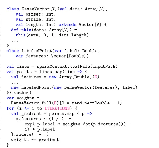
Fig. 1. Demo Spark program of ScalaLogistic Regression. It is an iterative machine learning application which caches the train-set data in memory. The top-level UDT of cached data objects isLabeledPoint.
An additionalLabeledPointobject is created for each data point to package its feature vector and label value together.
To eliminate disk I/O for the subsequent iterative computation, LR uses the cache operation to cache the resultingLabeledPointobjects in the memory. For a large input dataset, this cache may contain a massive number of objects.
After generating a random separating plane (lines 18-19), it iteratively runs another mapfunction and areducefunction to calculate a new gradient (lines 20–26). Here each call of this mapfunction will create a newDenseVectorobject. These intermediate ob-jects will not be used any more after executing the reduce function. Therefore, if the aforementioned cached data leaves little space in the memory, then GC will be fre-quently run to reclaim the space occupied by the intermediate objects and make space for newly generated ones. Note that, after running a number of minor GCs, JVM would run a full GC to reclaim spaces occupied by the old objects. However, such highly ex-pensive full GCs would be nearly useless because most cached data objects should not be removed from the memory.
[image:5.612.129.395.85.333.2]0 10 20 30 40 50 60
20GB 30GB 40GB
Time(s)
JVM Heap Size
Compute Time GC Time
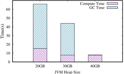
Fig. 2. Total execution time and GC time of Spark LR with different JVM heap sizes, running in Spark local mode (single JVM process). The input train-set data are 10GB randomly generated 10-dimension labeled feature vectors.
...
i
features label
double
Reference
Cached RDD:Array[LabeledPoint]
Array byte
Cached RDD:Array[byte]
label data(0) data(1) ... data(D-1) int
offset data
stride lenghth LabeledPoint DenseVector[Double]
Array[double] Spark
Deca
In Memory Data Objects
In Memory Bytes Matchup
Fig. 3. The cached RDD data layout of Spark LR in both the original version and the Deca transformed version. EachLabeledPointobject (with its contained objects) stores all raw data in onedoublefield, three
int fields and adouble array field. In the Deca version, the data of oneLabeledPointobject occupy a contiguous memory region that contains20 + 8×Dbytes.
the heap can contain all the objects, and hence there are only a few minor GCs, whose cost is negligible.
2.3. Life-time based Memory Management
[image:6.612.178.432.101.253.2] [image:6.612.172.446.302.502.2]1 def computeGradient() = {
2 val result = new Array[Double](D)
3 var offset = 0
4 while(offset < block.size) {
5 var factor = 0.0
6 val label = block.readDouble(offset)
7 offset += 8
8 for (i <- 0 to D) {
9 val feature = block.readDouble(offset)
10 factor += weights(i) * feature
11 offset += 8
12 }
13 factor = (1 / (1 + exp(-label * factor)) - 1) * label
14 offset -= 8 * D
15 for (i <- 0 to D) {
16 val value = block.readDouble(offset) 17 result(i) = result(i) + feature * factor
18 offset += 8
19 }
20 }
21 result
22 }
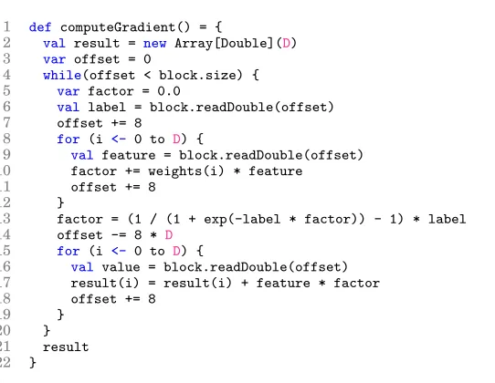
Fig. 4. A transformed source code fragment ofLogistic Regression.
the unnecessary object headers and object references. This compact layout would not only minimize the memory consumption of data objects but also dramatically reduce the overhead of GC, because GC only needs to trace a few byte arrays instead of a huge number of UDT objects. One can see that the size of each byte array should not be too small or too large, otherwise it would incur high GC overheads or large unused memory spaces.
As an example, theLabeledPointobjects in the LR program can be transformed into byte arrays as shown in Figure 3. Here, all the reference variables (in orange color, such as featuresanddata), as well as the headers of all the objects are eliminated. All the cachedLabeledPointobjects are stored into byte arrays.
The challenge of employing such a compact layout is that the space allocated to each object is fixed. Therefore, we have to ensure that the size of an object would not exceed its allocated space during execution so that it will not damage the data layout. This is easy for some types of fields, such as primitive types, but less obvious for others. Code analysis is necessary to identify the change patterns of the objects’ sizes. Such an anal-ysis may have a global scope. For example, a global code analanal-ysis may identify that the featuresarrays of all theLabeledPointobjects (created in line 14 in Figure 1) actually have the same fixed sizeD, which is a global constant. Furthermore, thefeaturesfield of aLabeledPointobject is only assigned in theLabeledPointconstructor. Therefore, all theLabeledPointobjects actually have the same fixed size. Another interesting pat-tern is that in Spark applications, objects in cached RDDs or shuffle buffers are often generated sequentially and their sizes will not be changed once they are completely generated. Identifying such useful patterns by a sophisticated code analysis is neces-sary to ensure the safety of decomposing UDT objects and storing them compactly into byte arrays.
[image:7.612.124.395.85.295.2]have the same lifetime, so they are stored in the same container. The byte arrays can be allocated on or off the JVM heap. When a container’s lifetime comes to an end, in the on-heap implementation, we simply release all the references of the byte arrays in the container, then the GC can reclaim the whole space occupied by the massive amount of objects. In the off-the-heap implementation, the memory space of a container can simply be released at the end of its lifetime.
Deca extracts information of programs by using intra-procedural analysis, decom-poses the UDTs and then modifies the application programs by replacing the bytecodes of object creation, field access and UDT methods with new codes that directly write and read the byte arrays. Finally, the converted programs will be submitted to Spark for execution.
In Figure 4, we illustrate the optimized code corresponding to the gradient com-putation code in lines 21–24 of Figure 1. While the codes produced by Deca are JVM bytecodes, we provide the equivalent Scala code here to illustrate the logic of the trans-formed LR code.
2.4. Technical scope of Deca
So far, we only implemented the prototype of Deca on Spark Core. However, the opti-mization techniques of Deca can also be used in other big data processing frameworks as long as they satisfy the assumption of Deca. Roughly speaking, we assume that most long-living objects of a job can be placed into containers, which have pre-determined lifetimes. Some other open-source frameworks also fulfill this assumption, likeHadoop, Storm, andGraphX, hence they can also be modified to benefit from Deca’s design. Fur-ther discussions of this issue can be found in Section 9.
3. UDT CLASSIFICATION ANALYSIS 3.1. Data-size and Size-type of Objects
To allocate enough memory space for objects, we have to compute the object sizes and their change patterns during runtime. Due to the complexity of object models, to accu-rately compute the size of a UDT, we have to dynamically traverse the runtime object reference graph of each target object and compute the total memory consumption. Such a dynamic analysis is too costly at runtime, especially with a large number of objects. Therefore we opt for static analysis which only uses static object reference graphs and would not incur any runtime overhead. We define thedata-sizeof an object to be the sum of the sizes of the primitive-type fields in its static object reference graph. An ob-ject’s data-sizeis only an upper bound of the actual memory consumption of its raw data, if one considers the cases with object sharing.
To see if UDT objects can be safely decomposed into byte sequences, we should ex-amine how their data-sizes change during runtime. There are two types of UDTs that can meet the safety requirement: 1) the data-sizes of all the instances of the UDT are identical and do not change during runtime; or 2) the data-sizes of all the instances of the UDT do not change during runtime. We call these two kinds of UDTs asStatic Fixed-Sized Type (SFST)andRuntime Fixed-Sized Type (RFST)respectively.
The objective of the UDT classification analysis is to generate theSize-Typeof each target UDT according to the above definitions. As demonstrated in Figure 3, Deca decomposes a set of objects into primitive values and store them contiguously into compact byte sequences in a byte array. A safe decomposition requires that the original UDT objects are either of an SFST or an RFST. Otherwise the operations that expand the byte sequences occupied by an object may overwrite the data of the subsequent objects in the same byte array. Furthermore, as we will discuss later, an SFST can be safely decomposed in more cases than an RFST. On the other hand, most objects that do not belong to an SFST or an RFST will not be decomposed into byte sequences in Deca. In Section 5, we will discuss the objects which belong to VST, but can still be decomposed subject to some restrictions. Apparently, to maximize the effect of our approach, we should avoid overestimating the variability of the data-size of the UDTs, which is the design goal of our following algorithms.
3.2. Local Classification Analysis
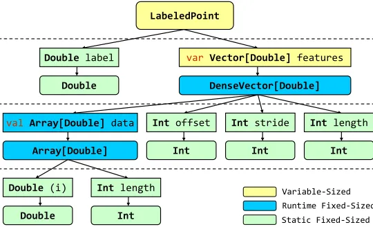
The local classification algorithm analyzes an UDT by recursively traversing its type dependency graph. For example, Figure 5 illustrates the type dependency graph of LabeledPoint. The size-type ofLabeledPointcan be determined based on the size-type of each of its fields.
Algorithm 1 shows the procedure of the local classification analysis. The input of the algorithm is anannotated typethat contains the information of fields and methods of the target UDT. Because the objects referenced by a field can be of any subtype of its declared type, we use a type-set to store all the possible runtime types of each field. The type-set of each field is obtained in a pre-processing phase of Deca by using the points-to analysis [Lhot ´ak and Hendren 2003] (see Section 6).
In lines 1–2, the algorithm first determines whether the target UDT is a recursively-defined type. It builds the type dependent graph and searches for cycles in the graph. If a cycle is found, the algorithm immediately returns recursively-defined type as the final result.
Two indirect-recursive functions, AnalyzeType (lines 4–22) and AnalyzeField (lines 23–34), are used to further determine the size-type of the target UDT. The stop condi-tion of the recursion is when the current type is a primitive type (line 5). We treat each array type as having a length field and an element field. Since different instances of an array type can have different lengths, arrays with static fixed-sized elements will be considered as an RFST (lines 8–9).
We define a total ordering of the variability of the size-types (except the recursively-defined type) as follows: SF ST < RF ST < V ST. Based on this order, the size-type of each UDT is determined by its field that has the highest variability (lines 12–20). Furthermore, each field’s final size-type is determined by the type with the highest variability in its type-set. But a non-final field of an RFST will be finally classified as VST, because the same field can possibly point to objects with different data-sizes (lines 28-29). Consider that whenever we find a VST field, the top-level UDT must also be classified as a VST. In this case, the function can immediately returns without further traversing the graph.
We take the typeLabeledPointin Figure 1 as a running example. In Figure 5, every field has a type-set with a single element and the declared type of each filed is equal to its corresponding runtime type except that the features field has a declared type (Vector), while its runtime type is DenseVector. Moreover, for a more sophisticated implementation of logistic regression with high-dimensional data sets, the features field can have bothDenseVectorandSparseVectorin its type-set.
ALGORITHM 1:Local classification analysis.
Input :The top-level annotated typeT;
Output:The size-type ofT;
1 build the type dependency graphGforT;
2 ifGcontains the circle paththen returnRecurDef; 3 else returnAnalyzeType(T);
4 FunctionAnalyzeType(targ)
5 iftargis a primitive typethen returnStaticFixed; 6 else iftargis an array typethen
7 fe←array element field oftarg; 8 ifAnalyzeField(fe)=StaticFixedthen 9 returnRuntimeFixed;
10 else returnVariable;
11 else
12 result←StaticFixed;
13 foreachfieldfof typetargdo
14 tmp←AnalyzeField(f);
15 iftmp=Variablethen returnVariable; 16 else iftmp=RuntimeFixedthen
17 result←RuntimeFixed;
18 end
19 end
20 returnresult;
21 end
22 end
23 FunctionAnalyzeField(farg) 24 result←StaticFixed;
25 foreachruntime typetinfarg.getT ypeSetdo 26 tmp←AnalyzeType(t);
27 iftmp=Variablethen returnVariable; 28 else iftmp=RuntimeFixedthen
29 iffargis notfinalthen returnVariable; 30 elseresult←RuntimeFixed;
31 end
32 end
33 returnresult;
34 end
field (i.e. label) and a field of the Vector type ( i.e. features). Therefore, the size-type of LabeledPoint is determined by the size-type of features, i.e. the size-type of DenseVector. It contains four fields: one of the array type and other three of the prim-itive type. Thedatafield will be classified as an RFST but not a VST due to its final modifier (valin Scala). Furthermore, theDenseVectorobjects assigned tofeaturescan have differentdata-sizevalues because they may contain different arrays. Therefore, bothfeaturesandLabeledPointbelong to VST.
3.3. Global Classification Analysis
LabeledPoint
Variable-Sized Runtime Fixed-Sized Static Fixed-Sized
DenseVector[Double] var Vector[Double] features
Array[Double] val Array[Double] data
Double label
Double
Int offset
Int
Int stride
Int
Int length
Int
Double (i)
Double
Int length
Int
Fig. 5. An example of the local classification.LabeledPointin Spark LR is classified asVariable-Sized Type.
data-sizevalues. Therefore it mistakenly classifies it as a VST, which can not be safely decomposed.
Furthermore, the local classifier assumes that theDenseVector objects contain ar-rays (features.data) with different lengths. Even if we change the modifier offeatures fromvartoval, i.e, only allowing it to be assigned once, the local classifier still consid-ers it as an RFST rather than an SFST.
For UDTs that are categorized as RFST or VST, we further propose an algorithm to refine the classification results via global code analysis on the relevant methods of the UDTs. To break the assumptions of the local classifier, the global one uses code anal-ysis to identify init-only fields and fixed-length array type according to the following definitions.
Init-only field. A field of a non-primitive typeTisinit-only, if, for each object, this field will only be assigned once during the program execution.1
Fixed-length array types. An array typeAcontained in the type-set of fieldfis a fixed-lengtharray type w.r.t.fif all theAobjects assigned tofare constructed with iden-tical length values within a well-defined scope, such as a single Spark job stage or a specific cached RDD. An example of symbolized constant propagation is shown in Figure 6. Here, array is constructed with the same length for whateverfoo() returns. The fixed-length array types with its element fields being SFST (or RFST) can be refined to SFST (or RFST).
1 val a = input.readString().toInt() // a == Symbol(1)
2 val b = 2 + a - 1 // b == Symbol(1) + 1
3 val c = a + 1 // c == Symbol(1) + 1
4 if (foo()) array = new Array[Int](b) 5 else array = new Array[Int](c) 6 // array.length == Symbol(1) + 1
Fig. 6. An example of the symbolized constant propagation.Symbol(1)is theint value read from the external data source at line 1. After symbolized constant propagation, Deca can determine that allint
array instances created at line 4 and 5 have the same length (Symbol(1) + 1).
1We always treat the array element fields as non init-only, otherwise the analysis needs to trace the element
[image:11.612.172.442.94.258.2]ALGORITHM 2:Global classification analysis.
Input :The top-level non-primitive typeT; The locally-classified size-typeSlocal; Call graph of the current analysis scopeGcall;
Output:The refined size-type ofT;
1 ifSRefine(T, Gcall)then returnStaticFixed;
2 else ifSlocal=RuntimeFixedorRRefine(T, Gcall)then 3 returnRuntimeFixed;
4 else returnVariable;
ALGORITHM 3:Static fixed-sized type refinement:SRefine(targ, garg)
1 FunctionSRefine(targ, garg)
Input :A non-primitive typetarg; A call graphgarg;
Output:trueorfalsethattarg’s size-type can be refined toStaticFixed; 2 foreachfieldfof typetargdo
3 foreachruntime typetinf.getT ypeSetdo
4 iftis not a primitive typeandnotSRefine(t, garg)then returnfalse;
5 end
6 end
7 iftargis an array typeandtargis notFixed-Lengthin call graphgargthen return false;
8 else returntrue; 9 end
In Figure 1, thefeatures field is only assigned in the constructor of LabeledPoint (lines 1–8), and the length offeatures.datais a global constant valueD (lines 14-16). Thus, the size-class ofLabeledPointcan be refined to SFST.
Algorithm 2 shows the procedure of the global classification. The input of the algo-rithm is the target UDT and the call graph of the current analysis scope. The refine-ment is done based on the following lemmas.
LEMMA3.1 (SFST REFINEMENT). An array type that is an RFST or a VST can be refined to an SFST if and only if for every array type in the type dependent graph, the followings are true:
(1) it is a fixed-length array type; and
(2) every type in the type-set of its element field is an SFST.
LEMMA3.2 (RFST REFINEMENT). An array type that is a VST can be refined to an RFST if and only if:
(1) every type in the type-sets of its fields is either an SFST or an RFST; and (2) each field with an RFST in its type-set is init-only.
The call graph used for the analysis is built in the pre-processing phase (Section 6). The entry node of the call graph is the main method of the current analysis scope, usually a Spark job stage, while all the reachable methods from the entry node as well as their corresponding calling sequences are stored in the graph.
ALGORITHM 4:Runtime fixed-sized type refinement:RRefine(targ, garg)
1 FunctionRRefine(targ, garg)
Input :A non-primitive typetarg; A call graphgarg;
Output:trueorfalsethattarg’s size-type can be refined toRuntimeFixed; 2 foreachfieldfof typetargdo
3 analyze f ield←false;
4 foreachruntime typetinf.getT ypeSetdo
5 iftis not a primitive typeandnotSRefine(t, garg)then
6 ifRRefine(t, garg)then
7 analyze f ield←true;
8 else returnfalse;
9 end
10 end
11 ifanalyze f ieldandfis notInit-Onlyin call graphgargthen returnfalse;
12 end
13 returntrue; 14 end
these objects are created). If all the length values used in all these allocation sites are equivalent,Ais of fixed-length w.r.t.f.
In line 11 of Algorithm 4, we use the following rules to identify init-only or non-init-only fields: 1) a final field is init-non-init-only; 2) an array element field is not init-non-init-only; 3) in addition, a field is init-only if it will not be assigned in any method in the call graph other than the constructors of its containing type, and it will only be assigned once in any constructor calling sequence.
3.4. Phased Refinement
In a typical data parallel programming framework, such as Spark, each job can be divided into one or more executionphases, each consisting of three steps: (1) reading data from materialized (on-disk or in-memory) data collectors, such as cached RDD, (2) applying an UDF on each data object, and (3) emitting the resulting data into a new materialized data collector. Figure 7 shows the framework of a job in Spark. It consists one or more top-level computation loops, each reads data object from its source, and writes the results into the sink. Every two successive loops are bridged by a data collector, such as an RDD or a shuffle buffer.
We observe that the data-sizes of object types may have different levels of variability at different phases. For example, in an early phase, data would be grouped together by their keys and their values would be concatenated into an array whose type is a VST at this phase. However, once the resulting objects are emitted to a data collector, e.g. a cached RDD, the subsequent phases might not reassign the array fields of these ob-jects. Therefore, the array types can be considered as RFSTs in the subsequent phases. We exploit this phenomenon to refine a data type’s size-class in each particular phase of a job, which is calledphased refinement. This can be achieved by running the global classification algorithm for the VSTs on each phase of the job.
4. LIFETIME-BASED MEMORY MANAGEMENT 4.1. The Spark Programming Framework
1 // The first loop is the input loop.
2 var source = stage.getInput() 3 var sink = stage.nextCollection() 4 while (source.hasNext()) { 5 val dataIn = source.next()
6 ...
7 val dataOut = ... 8 sink.write(dataOut)
9 }
10 // Optional inner loops
11 source = sink
12 sink = stage.nextCollection() 13 while (source.hasNext()) {...}
14 ...
15 // The last loop is the output loop
16 source = sink
17 sink = stage.getOutput() 18 while (source.hasNext()) {...}
Fig. 7. A typical task template of the Spark job stage. It consists one or more top-level computation loops, each reads data object from its source, and writes the results into the sink. Every two successive loops are bridged by a data collector, such as an in-memory RDD block or a shuffle buffer.
While Spark supports many operators, the ones most relevant for memory man-agement are some key-based operators, including reduceByKey, groupByKey, join and sortByKey (analogues of GroupBy-Aggregation, GroupBy, Inner-Join and OrderBy in SQL). These operators process data in the form of Key-Value pairs. For example, reduceByKeyandgroupByKeyare used for: 1) aggregating allValues with the sameKey into a singleValue; 2) building a completeValuelist for eachKeyfor further processing. Furthermore, these operators are implemented using data shuffling. The shuffle buffer stores the combined value of each Key. For example, for the case ofreduceByKey, it stores a partial aggregate value for each Key, and for the case ofgroupByKey, it stores a partial list ofValueobjects for each Key. When a newKey-Valuepair is put into the shuffle buffer, eager combining is performed to merge the newValuewith the combined value.
For each Spark application, a driver program negotiates with the cluster resource manager (e.g. YARN [Vavilapalli et al. 2013]), which launches executors (each with fixed amount of CPU and memory resource) on worker machines. An application can submit multiple jobs. Each job has severalstagesseparated by data shuffles and each stage consists of a set of tasks that perform the same computation. Each executor occupies a JVM process and executes the allocated tasks concurrently in a number of threads.
4.2. Lifetimes of Data Containers in Spark
In Spark, all objects are allocated in the running executors’ JVM heaps, and their ref-erences are stored in three kinds ofdata containers described below. A key challenge for Deca is deciding when and how to reclaim the allocated space. In thelifetime anal-ysis, we focus on the end points of the lifetime of the object references. The lifetime of an object ends once all its references are dead.
Cache blocks. In Spark, each RDD has an object that records its data source and the computation function. Only the cached RDDs will be materialized and retained in memory. A cached RDD consists of a number of cache blocks, each being an array of objects. The lifetimes of cached RDDs are explicitly determined by the invocations of cache() andunpersist() in the applications. Whenever a cached RDD has been “unpersisted”, all of its cache blocks will be released immediately. For non-cached RDDs, the objects only appear as local variables of the corresponding computation functions and hence are also short-living.
Shuffle buffers. A shuffle buffer is accessed by two successive phases in a job: one cre-ates the shuffle buffer and puts data objects into it, while the other reads out the data for further processing. Once the second phase is completed, the shuffle buffer will be released.
With regard to the lifetimes of the object references stored in a shuffle buffer, there are three situations. (1) In a sort-based shuffle buffer, objects are stored in an in-place sorting buffer sorted by the Key. Once object references are put into the buffer, they will not be removed by the subsequent sorting operations. Therefore, their lifetimes end when the shuffle buffer is released. (2) In a hash-based shuffle buffer with a reduceByKeyoperator, theKey-Value pairs are stored in an open hash table with the Key object as the hash key. Each aggregate operation will create a new Valueobject while keeping theKeyobjects intact. Therefore aValueobject reference dies upon an aggregate operation over its corresponding Key. (3) In a hash-based shuffle buffer with a groupByKeyoperator, a hash table stores a set of Key objects and an array ofValueobjects for eachKey. The combining function will only append Valueobjects to the corresponding array and will not remove any object reference. Hence, the references will die at the same time as the shuffle buffer. Note that these situations cover all the key-based operators in Spark. For example,aggregateByKey and join are similar to reduceByKey and groupByKey respectively. Other key-based operators are just extensions of the above basic operators and hence can be handled accordingly.
4.3. Data Containers in Deca
As discussed above, object references’ lifetimes can be bound with the lifetimes of their containers. Deca builds a data dependent graph for each job stage by points-to analy-sis [Lhot ´ak and Hendren 2003] to produce the mapping relationships between all the objects and their containers. Objects are identified by either their creation statements if they are created in the current stage, or their source cached blocks if they are read from cached blocks created by the previous stage.
However, an object can be assigned to multiple data containers. For example, if ob-jects are copies between two different cached RDDs, then they can be bound to the cached blocks of both RDDs. In such cases, we assign a soleprimary containeras the owner of each data object. Other containers are treated assecondary containers. The object ownership is determined based on the following rules:
(1) Cached RDDs and shuffle buffers have higher priority of data ownership than UDF variables, simply due to their longer expected lifetimes.
(2) If there are objects assigned to multiple high-priority containers in the same job stage, the container created first in the stage execution will own these objects.
In the rest of this subsection, we present how data are organized within the primary and secondary containers under various situations.
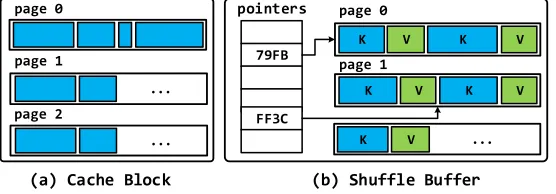
page 0
79FB
FF3C pointers
... page 1
K V K
... V
(a) Cache Block (b) Shuffle Buffer
page 0
page 1 ...
K V
K V K V
page 2
Fig. 8. Memory layouts of primary containers in Deca’s memory manager.
into consecutive byte segments, one for each top-layer object. Each of such segment can be further split into multiple segments, one for each lower-layer object, and so on. The page size is chosen to ensure that there is only a moderate number of pages in each executor’s JVM heap so that the GC overhead is negligible. On the other hand, the page size should not be too large either, so that there would not be a significant unused space in the last page of a container.
For each data container, a group of pages are allocated to store the objects it owns. Deca uses a page-info structure to maintain the metadata of each page group. The page-info of each page graph contains: 1)pages, a page array storing the references of all the allocated pages of this page group; 2)endOffset, an integer storing the start offset of the unused part of the last page in this group; 3)curPageandcurOffset, two integer values that store the progress of sequentially scanning, or appending to, this page group.
4.3.2. Primary Container.The way how Deca stores objects in their primary container depends on the type of the container:
UDF variables. Deca does not decompose objects owned by UDF variables. These ob-jects do not incur significant GC overheads, because: (1) the obob-jects only referenced by local variables are short-living objects and they belong to the young generation, which will be reclaimed by the cheap minor GCs; (2) the objects referenced by the function object fields may be promoted to the part of old generation, but the total number of these objects in a task is relatively small in comparing to the big input dataset.
Cache blocks. Deca always decomposes the SFST or RFST objects and stores their raw data bytes in the page group of a cache block. While cache blocks are designed to be immutable for the purpose of fault tolerance, VST objects can also be decomposed based on the type-set of fields. Figure 8(a) shows the structure of a cache block of a cached RDD, which contains decomposed objects.
A task can read objects from a decomposed cache block created in a previous phase. If this task changes the data-sizes of these objects, Deca has to re-construct the objects and release the original page group. To avoid thrashing, when such re-construction happens, Deca will not re-decompose these objects again even if they can be safely decomposed in the subsequent phases.
[image:16.612.169.447.96.193.2]However, the pointer array can be avoided for a hash-based shuffle buffer with both the Key and the Valuebeing of primitive types or SFSTs. This is because we can deduce the offsets of the data within the page statically.
As we discussed in Section 4.2, for a hash-based shuffle buffer with a GroupBy-Aggregation computation, a combining operation would kill the old Value object and create a new one. Therefore,Valueobjects are not long-living and frequent GC of these objects are generally unavoidable. However, if the Value object is of an SFST, then we can still decompose it and whenever a new object is generated by the combining operation, we can just reuse the page segment occupied by the old object, because the old and the new objects are of the same size. Doing this would save the frequent GC caused by these temporaryValueobjects.
When the working set size is larger than the available memory space of an executor, Spark moves part of its data out of the memory. For cached RDDs, Spark uses the LRU strategy to select the cache blocks for eviction. The evicted data will be directly discarded or swapped to the local disk according to the user-specifiedstorage-level. For shuffles, Spark always spills the partial data into temporary files, and merges them into final files at the end of task executions.
For cached RDDs, Deca modifies the original LRU strategy to evict page groups rather than cache blocks. Accessing in-page data through either page-infos or point-ers will refresh the corresponding page group’s recently-used counter. Spark serializes cache block data before write them into disk files, or transfer them through network for non-local accesses. In Deca, the decomposed data bytes can be directly used for disk and network I/O.
For shuffles, like Spark, Deca sorts the pointers before spilling, and writes the spilled data into files according to the order of the pointers. If a shuffle buffer has only pointers that reference page segments, Deca does not spill these pointers because normally they only occupy a small memory space. It pauses the shuffling and triggers the cache block eviction to make enough room. Deca uses a small memory space (normally only one page) to merge sorted spilled files. Once the merging space is fully filled, the merged data will be flushed to the final output file.
4.3.3. Secondary Container.There are common patterns of multiple data containers sharing the same data objects in Spark programs, such as: 1) manipulating data ob-jects in cache blocks or shuffle buffers through UDF variables; 2) copying obob-jects be-tween cached RDDs; 3) immediately caching the output objects of shuffling; 4) imme-diately shuffling the objects of a cached RDD.
If a secondary container is UDF variables, it will be assigned pointers to page seg-ments in the page group of the objects’ primary container. Otherwise, Deca stores data in the secondary container according to the following two different scenarios: (i) fully decomposable, where the objects can be safely decomposed in all the containers, and (ii) partially decomposable, where the objects cannot be decomposed in one or more containers.
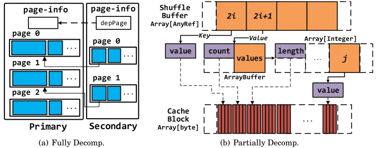
Fully decomposable.This scenario is illustrated in Figure 9(a). To avoid copy-by-value, a secondary container only stores the pointers to the page group owned by the primary, one for each object. Furthermore, we add an extra field,depPages, to the page-info of the secondary container to store the page-page-info(s) of the primary container(s).
··· page 0
··· page 1
Primary Secondary
···
page 2
depPage page-info page-info
··· page 0
page 1
···
(a) Fully Decomp.
j 2i 2i+1
Key Shuffle
Buffer
Array[AnyRef]
value
ArrayBuffer
Value Array[Integer]
value
... Cache
Block
Array[byte]
length count
values ...
(b) Partially Decomp.
Fig. 9. Examples of memory layout in Deca when data objects have multiple containers: (a) data objects can be decomposed in both of the primary container and the secondary container; (b) data objects can not be decomposed in its primary container (shuffle buffer) but are decomposable in its secondary container (cache block).
page group increments its reference counter by one, while destroying a container (and its page-info) does the opposite. Once the reference counter becomes zero, the space of the page group can be reclaimed.
Partially decomposable. In general, if the objects cannot be safely decomposed in one of the containers, then we cannot decompose them into a common page group shared by all the containers. However, if the objects are immutable or the modifications of objects in one container does not need to be propagated to the others, then we can decompose the objects in some containers and store the data in their object form in the non-decomposable containers. This is beneficial if the decomposable containers have long lifetimes.
Figure 9(b) depicts a representative example, where the output of agroupByKey op-erator, implemented via a hash-based shuffle buffer, is immediately cached in a RDD. Here,groupByKeycreates an array ofValueobjects in the hash-based shuffle buffer (see the middle of Figure 9(b)), and then the output is copied to the cache blocks. TheValue array is of a VST and hence cannot be decomposed in the shuffle buffer. However, in this case, the shuffle buffers would die after the data are copied to the cache blocks, and the subsequent modifications of the objects in the cache blocks do not need to be propagated back to the shuffle buffers. Therefore, as shown in Figure 9(b), we can safely decompose the data in the cache blocks, which have a long lifetime, and hence significantly reduce the GC overhead.
5. DECOMPOSITION OF VST AND FIELD-ORIENTED MEMORY PAGES 5.1. Decomposition of VST
In the previous sections and also in paper [Lu et al. 2016], only decomposing of SFST and RFST objects are considered. The key reason we do not decompose a VST object is that the memory manager cannot safely allocate a fixed space for it due to its variable size. Over-allocating space to account for the maximum possible size of a VST object would incur prohibitive waste of memory space, especially when the sizes of the objects of the same VST vary a lot.
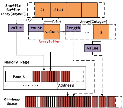
[image:18.612.118.498.98.247.2]Memory Page
Page k
··· ···
Off-heap Space
j 2i 2i+1
Key Shuffle
Buffer Array[AnyRef]
value
ArrayBuffer
Value Array[Integer]
value length count
values ...
[image:19.612.202.417.90.280.2]Address
Fig. 10. The memory layout of data containers for VST decomposition
typical VST used in a groupByKeyoperator. As mentioned in Section 4.3.1, groupByKey creates an array of Value objects in a hash-based shuffle buffer (see the middle of Figure 10). The Value objects whose keys have the same hash values are put into Values, which is an array. When the current array is full, a new array object with a larger size is created and used to replace the old one.
This means that JVM actually creates several fixed-size objects during the lifetime of a VST object. Deca makes use of this property, and decomposes each of such fixed-size objects. If we store these objects in the heap, it would result in frequent (but light-weight) GCs. To avoid this overhead, Deca stores a decomposed VST object in the off-heap space by usingsun.misc.Unsafeto allocate the necessary space. We maintain a pointer in the memory page to store the address of the decomposed object in the off-heap space. When JVM creates a new object caused by a size change of the VST object, Deca frees the off-heap space of the old object via Unsafe and allocates the necessary off-heap space for the new one. The address in the memory page would be updated accordingly. Note that to replace the old object with a new one, if the original program contains the copy statements, such as the array mentioned above, we copy the original bytes to new space additionally. This technique works only if the VST object is appropriately encapsulated as stated in the following lemma.
LEMMA5.1 (SAFEVST). The object of a VST can be safely decomposed if and only if all the following conditions hold:
(1) it is a private field;
(2) the new object reassigned to the field cannot be built outside of the class; and (3) the reference cannot be assigned to other fields.
O1
page 0
79FB
FF3C
pointers
...
page 1
K1
...
(a) Cache Block (b) Shuffle Buffer
page 0
page 1
O1
...O1
V1
...V1
O2
O2
O2 Field
_1
_2
···
Page
F000
F243
···
_3 F486
Mapping
Field
Key
V._1
···
Page
7F3C
8AA4
···
V._2 9FF2
Mapping
K3 K4
V2 V3 V4
[image:20.612.142.471.95.240.2]V2 V3 K2
Fig. 11. Memory layouts of data containers with field-oriented memory pages
Lastly, in Spark, cached RDDs are designed to be immutable to provide resiliency. In other words, objects stored in a cache container would never be updated, including their sizes, and hence can always be safely decomposed. Therefore, we only need to use the method introduced here to decompose the VST objects stored in shuffle buffers, which are mutable.
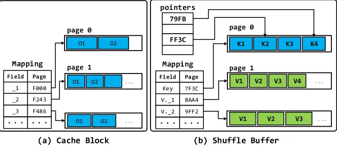
5.2. Field-oriented memory page
In the aforementioned design of memory pages, the UDT objects are stored one by one in a contiguous region. We call them object-oriented memory pages. When the data processing system caches a large number of intermediate objects, it is often desirable to compress the in-memory cached objects in order to maximize the usage of memory space and avoid swapping data to secondary disks. As the byte sequence of one UDT object contains different types of fields, its information entropyis high, which would have poor compression rates [Ziv and Lempel 1977], [Zhao et al. 2016].
To enhance the compression performance, we adopt field-oriented memory pages, which have a lower information entropy. A filed-oriented memory page only stores one field of a UDT. In other words, a UDT data object may be split and stored in a few memory pages. A mapping table is needed to manage the map from a field to the cor-responding memory pages. The mapping table can be produced by Algorithm 1 in local classification (Section 3). The algorithm runs recursively until it reaches a primitive type or an array type with primitive elements. We then allocate one page group to each of these fields. The name of this field and the address of the first allocated mem-ory page are put into the mapping table. Based on the mapping table, the structure of a field-oriented memory page is designed as follows.
Cache blocks. With the mapping table, the UDT objects are decomposed into several pages, as shown in Figure 11(a).
Shuffle buffers. Figure 11(b) shows the structure of a shuffle buffer. Besides the map-ping table, a pointer array is used for sorting or hashing operations, which is similar to the object-oriented memory pages. As the values of all the fields in a UDT have the same offset in their memory pages, the pointer array only needs to point to the first memory page. If the sorting operations compare other fields, they can also be accessed by the same offset.
array type with the memory pages of the element field storing the addresses of the actual off-heap spaces allocated to the arrays. If the array type is of SFST or RFST, we simply store the length field and the element field together into one memory page group instead of two, which will have little effect on the compression rate, but can simplify the operations on the arrays.
6. IMPLEMENTATION
We implement Deca based on Spark in roughly 12800 lines of Scala code. It consists of an optimizer used in the driver, and a memory manager used in every executor. The memory manager allocates and reclaims memory pages. It works together with the Spark cache manager and shuffle manager, which manage the un-decomposed data objects.
6.1. Optimizer in Deca
The optimizer analyzes and transforms the code of each job when it is submitted in the driver. Intuitively, Deca can be implemented as a standalone tool that transforms the compiled jar files of a Spark program before its execution. However, a Spark driver pro-gram may execute many jobs, each consisting of several stages separated by shuffles. The job submission will be implicitly triggered by anaction, such asreduce, which re-turns a value to the driver after running a UDF on a dataset. According to the results returned by the current job, the driver decides how to submit the next job.
A driver program can freely use the control statements (if/for/while) to control the computation. Therefore, it may submit different jobs with different input datasets and configuration parameters. A static optimization has to enumerate and process all the possible jobs by exhaustively exploring a large number of possible execution paths of the program, which is the well-known path explosionproblem [Raychev et al. 2015]. This is infeasible especially when the program has loop structures, which render the number of execution paths unbounded.
To address these challenges, we implement Deca in a hybrid way, which contains a static analyzer and a runtime optimizer. The static analyzer extracts a priori knowl-edge about the UDFs and UDTs of the target programs, which can be used to reduce the runtime optimization overheads. The runtime optimizer intercepts the submitted jobs at runtime, and optimizes each job before actually submitting it to the Spark plat-form. With this approach, Deca only optimizes the actually submitted jobs, and thereby completely eliminates the need for exploring all the execution paths.
6.2. Implementation of Optimizer
The Deca optimizer uses the Soot framework [Soot 2016] to analyze and manipulate the Java bytecode. The Soot framework provides a rich set of utilities that implement the classical program analysis and optimization methods.
In the pre-processing phase, Deca usesiterator fusion[Murray et al. 2011] to bun-dle the iterative and isolated invocations of UDFs into larger, hopefully optimizable code regions to avoid the complex and costly inter-procedural analysis. The per-stage call graphs and per-field type-sets are also built using Soot in this phase. Building per-phase call graphs will be delayed to the analysis phase if a phased refinement is necessary. In the analysis phase, Deca uses the methods described in Section 3 and Section 4 to determine whether and how to decompose particular data objects in their containers.
be further split into two sub-phases, decomposition and linking, which are described below.
6.2.1. Preprocessing.In this phase, Deca mainly performs iterator fusion to avoid inter-procedural analysis, which simplifies the analysis of Spark codes. Firstly, for the code of a Spark job, Deca builds a DAG based on RDD’s lineage graph. We make use of the implementation of DAGScheduler in Spark to divide the DAG built above into several stages according to the shuffle operations in the job. Each stage is represented as a stage-DAG. Secondly, Deca determines the hierarchical structure of the loop body, and uses Soot to generate the corresponding loop code. If cached RDDs exist in a stage, Deca generates new loop bodies to manage data objects in the cache buffer. Thirdly, we need to extract the UDFs to fill the loop body. By comprehending the semantic of the RDD and the operators likefilter, flatMapandmapValues, Deca uses Java reflec-tion to extract UDFs, and then inlines these UDFs in the loop body. Here, we need to guarantee the consistency between the return type of the previous UDF and next pa-rameter type of the next UDF. Finally, Deca generates aStage-Function-Class, which is similar to the class structure of UDF, and puts the loop body into this class. The detailed structure ofStage-Function-Classis displayed in Appendix A. Moreover, as for closures in UDF, they are created at the driver, and we choose to inject them into the final UDF object we have transformed.
6.2.2. Analysis.In this phase, in order to provide the important information of UDTs for code transformation, Deca uses Soot to perform points-to analysis in Stage-Function-Class, and then analyses the results of points-to analysis to guide UDT classification. Firstly, since the Stage-Function-Classafter performing iterator fusion is an independent class, which cannot be analyzed by soot-SPARK, a built-in pobuilt-ints-to analysis tool built-in Soot. To address the problem, Deca generates an entry method and an entry class linking to theStage-Function-Classtemporarily to make soot-SPARK applicable. We modify the implementation of soot-SPARK to realize full-context sensitivity, field sensitivity and object sensitivity. It is worth noting that soot-SPARK needs to load classes integrally, but the Stage-Function-Class may get in-volved in many irrelevant classes. So it is time-wasting to load all these classes. In our modification of soot-SPARK, we load classes, fields and methods incrementally dur-ing builddur-ing the call graph on the fly, hence the time overhead of UDT decomposition and code transformation can be reduced significantly. Thirdly, based on the result of points-to analysis, Deca invokes both local and global analysis to determine the types of UDTs in shuffle buffer and cache buffer. If we cannot decompose the UDT safely, Deca will simply terminate subsequent optimization.
For the safety of transformation, Deca also determines whether there is object shar-ing in the target stage program. There are three possible object sharshar-ing cases: inter-container sharing, intra-inter-container sharing, and intra-top-level-object sharing. Inter-container sharing is detected by the object-Inter-container mapping analysis described in Section 4.3. The pointer-based memory layout for this case is also described in Sec-tion 4.3.
6.2.3. Decomposition.In this phase, for the UDTs that can be decomposed safely, Deca transforms the UDT methods to directly accessing the bytes in the memory pages. Deca generates a synthesized class for each target UDT (calledSUDT). Logically, thethis reference of a decomposed UDT object is transformed to the start offset (the index of the first byte of its raw data) of its containing memory page. All the bytecode accessing the fields of this object are transformed to access the memory pages based on the ab-solute field offset (object start offset + relative field offset), the fields also include each field defined in the parent classes of the UDT. The offset computation depends on the raw data size of each UDT instance. In each SUDT, Deca synthesizes somestatic fields or methods to obtain the values of the data sizes of all the UDT fields. While the data sizes of the primitive type fields are defined in the official JVM specification, the sizes of fields of non-primitive types can be recursively obtained from the corre-sponding SUDTs. If a field’s data size can be determined statically, then it is stored as a global constant value in a static field in the corresponding SUDT. Otherwise, Deca synthesizes a static method of the SUDT to compute the data size at runtime. Sim-ilarly, for each UDT, Deca synthesizes some static fields or methods to provide the relative offsets of all the UDT fields in the SUDT. The relative offsets can be computed based on the data sizes and the ordering of the fields in the UDT definition. As an optimization technique, we reorder the UDT fields by putting the fields with statically determinable sizes in the front, and hence enable more fields’ offsets to be determined statically.
After doing the above on all the fields, Deca transforms the methods of the UDT into its SUDT. During the transformation, all the field accessing code in the methods are replaced with the array accessing code. At this point, transforming the UDT fields and UDT methods to the array accessing codes is similar to Facade [Nguyen et al. 2015]. What distinguishes Deca from Facade is that we flatten all the fields of a UDT in the synthesized class to realize a flat memory layout, and remove the references structure in UDT, which still exists in the transformed classes in Facade, so that the offset of each UDT instance or a field of the UDT instance can be computed accurately and statically.
The memory pages storing the decomposed objects can be stored in two ways in Deca: on-heap and off-heap. We can allocate the memory space for each page by creating an object on the heap. At the end of the lifetime of all the objects in the page, we simply discard the references to the page and rely on the GC to manage the space reclamation. The advantage of this method is its ease of implementation. It is convenient to define the memory page class with all the necessary data access methods and the allocation of memory space can be simply performed by instantiating the page objects. Further-more, as the number of memory pages are most likely to be relatively small, the GC overhead will be low.
The off-heap memory can be completely managed with Unsafe, which contains op-erations such as allocate(), put(), release(), etc. As managing the off-heap memory space will not incur any GC overhead, it is expected that using this approach in Deca has the lowest GC cost.
Another important thing to take into account is sharing information among the stages in a job. Some stages may need synthesized classes generated by previous stages to transform their own bytecode. So we cache the synthesized classes of all transformed stages if necessary.
Stage-Function-Class and detect which statement and reachable method referenced uses the synthesized classes, then traces the new site of the each synthesized class. If the new site of the synthesized class is included in the results provided by points-to analysis, it means that the objects of the synthesized class exist in a data container (shuffle buffer or cache buffer), or objects are only temporary. As for the temporary ob-jects of the synthesized classes, Deca creates temporary memory pages to store them. Since these temporary objects are only referenced by local variables and will be re-claimed by minor GCs, Deca creates and reclaim such temporary pages at the start and the end of a loop body respectively.
In Spark, every task processes data objects sequentially in each UDT object array in a loop. Since Deca allocates byte arrays for data caching and shuffling instead of object arrays as in vanilla Spark, we have to calculate the array index values in the loop based on the raw data sizes of each object in the optimized code. In fact, the array index variable stores the value of the start offset of the data object currently being processed. Base on these new array index values, Deca changes the code ofStage-Function-Class and other involved classes that uses the synthesized classes with the following steps: 1) remove the invocations of the UDT object constructors and directly write the initial values of the constructor parameters into the byte arrays based on the absolute field offset; 2) replace all the field accessing codes with the array accessing code; 3) replace each invocation of a UDT method with the corresponding SUDT method, and add the byte array and the start offset as the additional parameters of the invocation.
Finally, when the transformation of all the stages of a job finishes, Deca compresses Stage-Function-Class and all classes involved into a jar file, and transfers the jar file to each executor to ensure the job runs effectively. Then Deca creates a new RDD, injects a function object created by Stage-Function-Class into a new RDD for each stage, and resubmit the job that contains the DAG formed by the new RDDs.
Since executing an iterative application may involve submitting a massive amount of jobs to Spark, it is time consuming (and wasting) to repeat the aforementioned op-timization for every submitted job. To solve the problem, Deca stores in memory the RDD-DAG structure, the UDFs of each stage in the very first job, and the synthetic Stage-Function-Class of each stage. Before optimizing a stage, if Deca detects an equivalent stage (by comparing their RDD-DAG structure and UDFs) has already been optimized, it can simply reuse theStage-Function-Classstored in memory.
We present the optimized code corresponding to theStage-Function-Classof LR in Figure 20, which illustrates more details of Deca’s optimization.
7. EVALUATION
We use five nodes in the experiments, with one node as the master and the rest as workers. Each node is equipped with two eight-core Xeon-2670 CPUs, 64GB memory and one SAS disk, running RedHat Enterprise Linux 5 (kernel 2.6.18) and JDK 1.7.0 (with default GC parameters). We compare the performance of Deca with Spark 1.6. For serializing cached data in Spark, we use Kryo, which is a very efficient serializa-tion framework. All the experiments are repeated 5 times and we report the average execution time, garbage collection time and their standard deviation (SD).
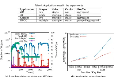
Table I. Applications used in the experiments
Application Stages Jobs Cache Shuffle
WC two single non aggregated LR single multiple static non KMeans two multiple static aggregated PR/CC multiple multiple static grouped/aggregated
1 100 10000 1x10⁶ 1x10⁸ 1x10¹⁰
0 500 1000 1500 2000 0 10 20 30 40 50 60 70 80 90 100
Number of Objects
Time of GC(s)
Time(s)
Spark-Tuple2 Spark-GC Deca-Tuple2 Deca-GC
(a) Live data object numbers and GC time.
0 1 2 3 4 5 6
50GB 100GB 150GB 50GB 100GB 150GB
Execution Time (1000s)
Data Size / Key Size Spark-exec
Deca-exec
0 1 2 3 4 5 6
10M 100M
Execution Time (1000s)
Data Size / Key Size
(b) Application execution time.
Fig. 12. Comparison of performance for the shuffle-onlyWordCountapplication of Spark and Deca.
200GB). For PR and CC, we use three real graphs: LiveJournal social network [Back-strom et al. 2006] (2GB), webbase-2001 [Boldi and Vigna 2004] (30GB) and a 60GB graph generated by HiBench [HiBench 2016]. The maximum JVM heap size of each executor is set to be 30GB for the applications with only data caching or data shuffling, and 20GB for those with both caching and shuffling.
7.1. Impact of Shuffling
WC is a two-stage MapReduce application with data shuffling between the “map” and “reduce” stages. We examine the lifetimes of data objects in the shuffle buffers with the smallest dataset. We periodically record the alive number of objects and the GC time with JProfiler 9.0. The result is shown in Figure 12(a). WC uses a hash-based shuffle buffer to perform eager aggregation, which is implemented in Tuple2. The number of Tuple2 objects, which fluctuates during the execution, can indicate the number of objects in shuffle buffers. While the number ofTuple2are also large in ”map” stage but decrease in shuffle in Deca. GCs are triggered frequently to release the space occupied by the temporary objects in the shuffle buffers.