Exploring the physical controls of regional patterns of flow duration curves – Part 4: A synthesis of empirical analysis, process modeling and catchment classification

www.hydrol-earth-syst-sci.net/16/4483/2012/ doi:10.5194/hess-16-4483-2012

© Author(s) 2012. CC Attribution 3.0 License.

Earth System

Sciences

Exploring the physical controls of regional patterns of flow duration

curves – Part 4: A synthesis of empirical analysis, process modeling

and catchment classification

M. Yaeger1, E. Coopersmith1, S. Ye2, L. Cheng3, A. Viglione4, and M. Sivapalan1,2

1_{Department of Civil and Environmental Engineering, University of Illinois at Urbana-Champaign, Urbana, IL, USA} 2_{Department of Geography, University of Illinois at Urbana-Champaign, Urbana, IL, USA}

3_{Water for a Healthy Country Flagship, CSIRO Land and Water, Canberra, ACT, Australia}

4_{Institute of Hydrology and Water Resources Management, Vienna University of Technology, Vienna, Austria}

Correspondence to: M. Yaeger ([email protected])

Received: 10 May 2012 – Published in Hydrol. Earth Syst. Sci. Discuss.: 6 June 2012 Revised: 19 September 2012 – Accepted: 5 November 2012 – Published: 26 November 2012

Abstract. The paper reports on a four-pronged study of the physical controls on regional patterns of the flow duration curve (FDC). This involved a comparative analysis of long-term continuous data from nearly 200 catchments around the US, encompassing a wide range of climates, geology, and ecology. The analysis was done from three different perspec-tives – statistical analysis, process-based modeling, and data-based classification – followed by a synthesis, which is the focus of this paper. Streamflow data were separated into fast and slow flow responses, and associated signatures, and both total flow and its components were analyzed to generate pat-terns. Regional patterns emerged in all aspects of the study. The mixed gamma distribution described well the shape of the FDC; regression analysis indicated that certain climate and catchment properties were first-order controls on the shape of the FDC. In order to understand the spatial patterns revealed by the statistical study, and guided by the hypothesis that the middle portion of the FDC is a function of the regime curve (RC, mean within-year variation of flow), we set out to classify these catchments, both empirically and through process-based modeling, in terms of their regime behavior. The classification analysis showed that climate seasonality and aridity, either directly (empirical classes) or through phe-nology (vegetation processes), were the dominant controls on the RC. Quantitative synthesis of these results determined that these classes were indeed related to the FDC through its slope and related statistical parameters. Qualitative synthe-sis revealed much diversity in the shapes of the FDCs even

within each climate-based homogeneous class, especially in the low-flow tails, suggesting that catchment properties may have become the dominant controls. Thus, while the mid-dle portion of the FDC contains the average response of the catchment, and is mainly controlled by climate, the tails of the FDC, notably the low-flow tails, are mainly controlled by catchment properties such as geology and soils. The regime behavior explains only part of the FDC; to gain a deeper un-derstanding of the physical controls on the FDC, these ex-tremes must be analyzed as well. Thus, to completely sep-arate the climate controls from the catchment controls, the roles of catchment properties such as soils, geology, topog-raphy etc. must be explored in detail.

1 Introduction

activities. We hypothesize that some function relates each hy-drologic signature, the FDC included, to both the climate and the landscape, thus connecting the variability of climate in-puts to the variability of runoff. This function can then be determined empirically, through the application of complex process-based models, or some combination thereof, both in detail for a small region via a process-based (Newtonian) ap-proach, or through a comparative, data-based (Darwinian) approach. On the basis of these analyses, unique functions can then be defined for regions of similar catchment and landscape properties. With this idea of regionalization based on clusters of similar behavior, the prediction of the FDC or any other hydrologic signature can be greatly improved in cases where this function is not easily determined, such as ungauged basins.

The FDC is a signature of the within-year variability of the runoff in a watershed and represents the relationship be-tween magnitude and frequency of streamflows at some lo-cation in the basin (Botter et al., 2008). Although the FDC is widely used in practice, and with much empirical knowledge in specific regions having been gained, the physical controls on the shape of the FDC are still not well understood (Yokoo and Sivapalan, 2011). Because of its wide usage and the sim-ple data demands on its construction, the FDC is an impor-tant catchment signature. In a rapidly changing world, such signatures can be used to track catchment responses to per-turbations, in addition to the more traditional application to analyze or interpret long-term catchment responses (Vogel and Fennessey, 1995). Improved understanding of the physi-cal processes controlling the shape of the FDC would allow for better comparisons of catchments across diverse regions as well as over long time periods for a single catchment. Ul-timately, an increased understanding of the controls on the FDC would enable better estimation and prediction of the re-sponse from ungauged catchments, as well as improving our ability to carry out hydrologic space-for-time substitutions when making predictions under change.

In the past, FDCs have been generally analyzed through purely graphical means (e.g., Vogel and Fennesy, 1994, 1995) or stochastically by fitting appropriate statistical distri-butions (e.g., Le Boutillier and Waylen, 1993; Castellarin et al., 2004, 2007). Recently, the stochastic approach has been augmented with a more process-based approach, wherein the different components of the catchment’s dynamic response are incorporated into stochastic models (Botter et al., 2007a, b, 2009; Muneepeerakul et al., 2010), thus allowing for a more complete picture of the streamflow variability of dif-ferent catchments. Their complete model contains many un-derlying physical properties of a catchment but still uses a Poisson assumption for the arrival of rainfall events, which enables an analytical solution to be obtained. The model is applied seasonally, and, since there is no carryover of soil moisture storage between seasons, the results are not appli-cable to the whole year. This may not be realistic in all cases, especially in regions that exhibit strong seasonal variations

of climate and water storage, and highlights the need for a more general framework, one for the entire year that captures within-year variations in climate and soil moisture storage.

The numerical study of Yokoo and Sivapalan (2011) fol-lowed this process-based framework with one important ex-ception: there is no Poisson assumption. Rather, their numer-ical water balance modeling framework uses precipitation data (either observed or synthetic) to both provide the ran-domness inherent in precipitation at the event scale and yet capture the seasonal variability of climate. Carryover of soil moisture storage across the year allows for antecedent soil moisture conditions to affect the runoff response of the catch-ment. As a result of this work, they hypothesized that the flow duration curve could be divided into three parts, or limbs. The upper limb corresponds to the fast flow response of a catchment to precipitation; the middle limb is related to the slow flow response of the catchment, and as such is a func-tion of the monthly regime curve; and the tail limb could be related to evaporation from variable saturated regions in the catchment impacting low flows. This insight, to separate the streamflow into fast flow and slow flow and look at the FDC the same way, provided the motivation for this four-pronged study, which was undertaken to further explore the possible physical controls on the FDC. While the Yokoo and Siva-palan work was mainly hypothetical and used synthetic in-puts to a hydrological model, the present four-pronged study that follows it is empirically based, using long-term continu-ous daily climate and streamflow data from about 200 catch-ments in the MOPEX database. Using this data, the possible controls on the FDC were explored from three angles: statis-tically to identify patterns, through the use of a simple physi-cally based model to separate climate and landscape controls, and through catchment classification to organize the patterns into classes.

The first angle of exploration was empirical (Cheng et al., 2012), and was accomplished by first separating total stream-flow (Q)into fast flow (Qf)and slow flow (Qu)and fitting

each of their duration curves as well as that of precipitation (P )to a mixed gamma distribution, which has three parame-ters:κ,θ, andα. The first two parameters – the shape param-eterκ, which affects the shape of the curve, and the scale pa-rameterθ, which stretches or shrinks the curve and is related to the magnitude of the variable in question – are embedded in the standard gamma distribution. However, for the dura-tion curves ofP andQf, as well asQof catchments in arid

the catchment, represented in the baseflow index (BI), are the dominant controls on the shape of the FDCs of Qand

Qu, while climate (precipitation) is the dominant control on

the shape of the FDC ofQf. However, this dominance was

by no means absolute, which meant that other factors may be controlling the shapes as well, and this in turn led to the modeling portion of the study as a way to further elucidate these other controlling factors.

The second angle of exploration involved top-down pro-cess modeling (Ye et al., 2012), using a simple two-stage hy-drologic model following the modeling framework outlined in Yokoo and Sivapalan (2011). The regime curve (RC) is used as the signature of comparison during the model cal-ibration since, as previously mentioned, the middle portion of the FDC, which connects the high flows to the low flows, is related to the RC, and both the FDC and the RC are nec-essary for understanding the catchment response. Where the base model failed to capture fully the shape of the RC, pro-cesses were added to the model in a systematic fashion, but always guided by the data. Controlling processes were then identified for each catchment, and, when plotted spatially, these also showed interesting regional patterns. As an ex-ample, phenology (vegetation-induced seasonality in stream-flow) and snowmelt processes dominated the northeast por-tion of the US, with both becoming less dominant towards the south and west. In some cases, however, very different catchments had the same controlling process. For instance, precipitation seasonality dominated in both the mountainous Pacific Northwest and in the flat peninsula region of Florida, highlighting the fact that dominant processes alone may not make catchments similar, and pointing towards a need for further classification of catchment response.

The third angle of exploration involved the development of a classification system using information readily obtained from the daily RC (Coopersmith et al., 2012). Unlike the pre-vious two studies, all 428 catchments in the MOPEX dataset were used in order have the highest possible variation in cli-mate and location, since most of the long-term hydrologic data in the US tend to be concentrated in the more humid, eastern half of the country. As with the modeling study, the RC was chosen as the signature of comparison instead of the FDC and for much the same reasons, with one addition: the RC contains much more easily interpretable information than does the FDC. This may indeed be one of the reasons the FDC is still not well-understood, even after much use and much study. From the RCs ofP, potential evaporation (Ep), Qand its componentsQfandQu, one can establish the

av-erage aridity and seasonality of the climate, as well as when

P andQpeak for a particular catchment. Using these four similarity indices and an objective function that minimized within-group variance, catchments were clustered along a decision tree until further splitting ceased when catchments within a terminal node were sufficiently similar or there was no further reduction in variability by splitting again. Over three-fourths of the catchments studied fell into only six

classes, with the first major distinction between catchments being seasonality. The eastern portion of the US experiences very low seasonality in precipitation, with a wet/dry seasonal pattern becoming more pronounced as one moves further west across the continent. Again, interesting regional pat-terns emerged when the catchment classes were displayed spatially. As with the model processes, the Northeastern US formed a different cluster than the Southeast, and the Mid-west US formed two major clusters, but this time the Pacific Northwest and Florida in the extreme Southeast fell into two different classes. This shows that while both regions experi-ence high seasonality inP (the dominant model process), the amount of rainfall each region receives (more overall in the NW,) as well as the timing of the wet season (in the NW it is out of phase withEp, while in FL it is in phase),

distin-guishes Florida from the Pacific NW. This analysis leads to the conclusion that there may be some connection between the results of each of these studies, and elucidation of this connection could lead to deeper insights into the controls on the FDC.

on this synthesis that a deeper understanding of the physical processes controlling the shape of the FDC can be gained.

This paper is divided into four sections. In Sect. 1, we have introduced the FDC, and the ideas of regionalization, similar-ity, and synthesis as a way to better understand the physical controls on the shape of the FDC. Section 2 describes the study site, data used, and the specific methods used in the synthesis, and Sect. 3 presents the results of the synthesis. In Sect. 4 the conclusions of the entire four-part study are sum-marized. We conclude with a discussion of the limitations of the study and a look towards future work that will overcome these limitations.

2 Data and methods

2.1 Study site and data description

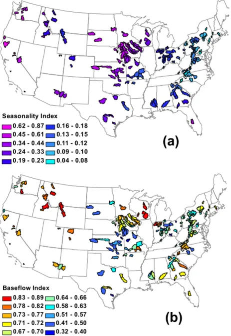
Out of the 428 catchments in the MOPEX database, 197 catchments were chosen for their long-term, continuous daily datasets. The data used in the present work (area-averaged daily precipitation, total streamflow, baseflow-separated streamflow, and potential evaporation, all in units of mm) were assembled into a processed database as part of the Hydrologic Synthesis Project (Sivapalan et al., 2011b; Brooks et al., 2011) and is freely available at http://voda.hwr. arizona.edu/mopex/. While the overall spatial distribution of these catchments covers the entire continental United States and therefore represents most of the climate and geographic variability found there, a majority of the catchments are lo-cated east of the Mississippi River (Fig. 1). In the empiri-cal, modeling, and classification studies, the common theme of emergent regional patterns in the spatial distribution of the gamma parameters, the dominant model processes, and the catchment classes provided visual evidence of some un-derlying organization. Clear spatial patterns are also seen in climate indicators such as the aridity index (Ep/P), which

exhibits the typical continental pattern of increasing aridity with increasing distance from the coast and with decreasing latitude in the Western US, as well as the seasonality index (Fig. 1a), adapted from Walsh and Lawler (1981) and defined here as

SI=

P365

i=1

Pi−

P365

i=1Pi

365

P365

i=1Pi

365

(1)

wherePi is the daily precipitation at each site. Less clear

is the spatial organization of catchment-related indices such as the baseflow index(Qu/Q), shown in Fig. 1b. Since the

baseflow index is related in large part to geology, which tends to vary at the local scale, its spatial pattern shows a more localized clustering compared to the climate indices, which tend to vary along a gradient.

Daily data from the processed MOPEX database were first normalized before being used in this study, with P

Baseflow Index 0.83 - 0.89 0.78 - 0.82 0.73 - 0.77 0.71 - 0.72 0.67 - 0.70

0.64 - 0.66 0.58 - 0.63 0.51 - 0.57 0.41 - 0.50 0.32 - 0.40 Seasonality Index

0.62 - 0.87 0.45 - 0.61 0.34 - 0.44 0.24 - 0.33 0.19 - 0.23

0.16 - 0.18 0.13 - 0.15 0.11 - 0.12 0.09 - 0.10 0.04 - 0.08

(a)

(b)

Fig. 1. Spatial patterns of seasonality index (a) and baseflow index (b) across the continental US.

normalized by the mean annual daily precipitation for the 54 yr time period, andQ,Qf, andQuall normalized by the

corresponding mean flow values for the same time period. The duration curves ofP,Q,Qf,Quanalyzed herein were

produced using the quantile method (Vogel and Fennessey, 1994); i.e., only data points corresponding to the 0.5, 1.0, 1.5, ..., 99.0, and 99.5 exceedance percentages from the 54 years of normalized daily data were considered. In addition to the processed daily time-series data, results from the first three parts of the four-part study described previously were used to create a database for the synthesis analysis. From the empirical analysis (Cheng et al., 2012), the fitted parameters of the mixed gamma distributionα,κ, andθ forP,Q,Qf,

andQufor each catchment were obtained. From the

previous two studies will also be used. These are calculated using the entire period of record by finding the average flow for each Julian day of the year, then smoothing with a 30-day circular moving average (see Coopersmith et al., 2012, for further details).

2.2 Synthesis methods

As discussed earlier, all the work done in these related stud-ies, including the present one, has been guided by the frame-work laid out in Yokoo and Sivapalan (2011), which is pre-sented visually in Fig. 2. This conceptual model was built on the partitioning idea outlined by L’vovich (1979), wherein

P is partitioned intoQfand catchment wetting (infiltration),

and this wetting is then further partitioned intoQuand

va-porization (ET). Thus the upper portion of the FDC, which represents the high flows that are exceeded rarely, is con-trolled by Qf, a simple function ofP. The middle portion

of the FDC, which represents the average flows, is controlled byQu, which is a function of the monthly flow regime. The

lower portion of the FDC, which represents the extreme low flows that are exceeded most of the time, may be a function of evaporation from saturated areas, among other things. In this framework, the RC, which contains the average flows experienced by a catchment throughout the year, forms the bridge between the low flows and the high flows in the FDC. Thus the results from the modeling and classification studies can be used to learn more about the physical controls on the FDC.

Because the middle limb of the FDC forms the connection between the extreme high flows and the extreme low flows, and is related to the average flow regime of a catchment, the slope of this portion of the FDC is often used in modeling and classification studies as a means of quantifying the shape of the FDC (Carillo et al., 2011; Sawicz et al., 2011; Yadav et al., 2007). The fitted gamma parameters also quantify the shape of the FDC, but they encompass all of the FDC, not just the middle portion. Since the middle part of the FDC re-lates to the RC and therefore the modeling and classification studies, it is included here as a way to synthesize the findings of these studies. From the three papers cited above, the slope of the flow duration curve is defined as

Slope_FDC=ln(Q0.33)−ln(Q0.66)

(0.66−0.33) (2)

whereQ0.33 andQ0.66 are the flow values exceeded 33 %

and 66% of the time, respectively. SinceP andQf are

ei-ther zero or some extremely small number (<0.001 mm) and usually exceeded at or less than 66 % of the time in nearly all the catchments, the slopes (as defined here) of these duration curves were not mathematically meaningful, and thus only the slopes only the slopes of theQandQuFDCs were used

for this analysis.

The three previous studies – empirical, modeling, and clas-sification – form three angles of what can conceptually be

Q_ucontrols the middle part

Q_fcontrols the upper part

Q_f: a simple

function of P

Q_u: a simple

function of monthly flow regime

Percent of Time Exceeded

Normalized

Daily Flow

Fig. 2. Conceptual model of the controls on the FDC (adapted

from Yokoo and Sivapalan, 2011); hereQfis the fast flow (surface

runoff) andQuis the slow flow (sub-surface runoff).

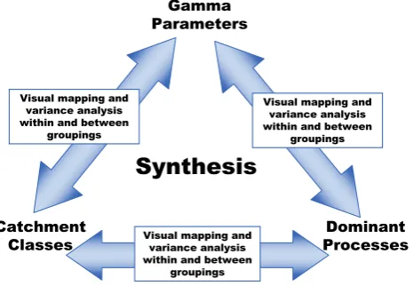
described as a synthesis “triangle” (Fig. 3). The parameters of the mixed gamma distribution form the apex of the trian-gle, and at the base, moving clockwise from the top, are the dominant model processes and the catchment classes. The goal of the synthesis analysis is to make connections be-tween each of these three angles, thus forming the “legs” and completing the triangle. To map the FDC to possible controlling processes, a two-stage analysis is conducted: for each leg of the synthesis triangle, a qualitative visual group-ing analysis is followed by a quantitative variability analysis. Additionally, because two of the legs of the triangle are de-rived from the RC, the synthesis analysis will zoom in on the middle portion of the FDC and the same visual group-ing and variability analysis will be performed on the slope of the FDCs sorted by both catchment class and dominant processes. Lastly, because of the regression relationship seen between the shape parameter of the mixed gamma distribu-tionκ and the baseflow and seasonality indices, the slope of the FDC will also be compared to these indices. Sinceκ rep-resents the entire FDC and the FDC slope reprep-resents just the middle portion of the FDC, a strong relationship may help clarify the underlying controls. Thus the analysis of the slope of the FDC builds on the three-way mapping outlined by the synthesis triangle.

The variability analysis must be done between sets of quantitative data (parameters of the mixed gamma distribu-tion, the slopes and quantiles of the FDCs) as well as be-tween sets of qualitative data (the dominant model processes and catchment classes). For the quantitative data, this is ac-complished by determining self-organizing behavior with a decision tree (Breiman et al., 1993). Consider a dataset of sizen, with varianceσ2. Next, partition that dataset intom

subsets, using an existing decision tree. Each subsetiof size

Si is characterized by a varianceσ_i2. Let a variance measure

Gamma Parameters

Synthesis

Catchment

Classes Visual mapping and variance analysis ProcessesDominant

within and between groupings

Visual mapping and variance analysis within and between

groupings Visual mapping and

variance analysis within and between

groupings

Fig. 3. Connections to be explored between the three aspects of the

FDC study.

σ2=

m

6

i=1Siσ 2

i

n . (3)

In essence, the average of the variance of each subset is cal-culated, weighted by the number of members of each subset. For the qualitative data, this is accomplished by determin-ing self-organization into distinct classes. Again, consider a dataset of sizen, which now is characterized bykdistinct, qualitatively described classes. Let the entropy of any group of that data be defined as

E= −₆k

j=1

pjlogkpj (4)

wherepj represents the proportion of the group of classj.

Equation (4) returns a value between 0 (minimum entropy, all elements within a set of the same class) and 1 (maximum entropy, equal proportions of a set of each of thekclasses). Next, partition the dataset of size ninto msubsets of size

Si, each with an entropyEi, calculated with Eq. (4). Let the

entropy of the data, using the partitions implied by the tree, analogous to Eq. (3), be calculated as follows:

E=

m

6

i=1 SiEi

n . (5)

If the variance measure calculated in Eq. (3) and the entropy calculated in Eq. (5) are lower than that of the entire dataset, we can conclude that the tree structure explains, in part, the variability of the parameters/classes we desire to map.

3 Results: three-way mapping and synthesis

3.1 Catchment classes and dominant processes

Figure 4 shows the FDCs of catchments in the four largest catchment classes, which together account for about two-thirds of all the catchments in the study, grouped within each class by dominant model process. The class LJ (low season-ality, wetter spring), which includes 68 catchments and en-compasses most of the Atlantic coast region of the US, and the class LWC (low seasonality, wetter winters), which cov-ers the southern Appalachian Mountain region and the south-ern Gulf states, show remarkably little difference between FDCs for high flows exceeded about 15–20 % of the time (Fig. 4c and d). The curves begin to diverge at the mid- to low-flow end, as well as at the extreme high flow end, but even there the range is less than that of the intermediate sea-sonality classes ISQJ and ITC, which include catchments in the Midwest from the humid Corn Belt region in Illinois and Iowa to the drier Plains regions south and west of the Corn Belt (Fig. 4a and b). Of note is that the catchments in these two intermediate seasonality classes are also where the sim-ple process model had difficulty in satisfactorily reproducing the regime curve (Ye et al., 2012), while the two dominant low-seasonality classes are largely made up of model process classes relating to forest and snow processes.

In Fig. 5 the grouping is reversed; here the FDCs of catch-ments in the four largest dominant model process classes, which together account for about half of all the catchments in the study, are grouped within by catchment classification. Again, we see two of these classes (b and c) have smaller range of FDC variability than the other two. A closer inspec-tion reveals that both (b) and (c) seem to taper at the top (largest flows) while (a) and (d) do not. Since the vertical axis of an FDC is on a log scale, any differences that appear small at this end are actually quite large, while differences between FDCs at the low end, which appear large, are actu-ally very small. It can be further noted that both (b) and (c) contain subsurface-influencedQf, and it may be due in part

10−3

10−2

10−1

100

101

102

(a) ISQJ

Flux (mm/d) / Q

ave

(mm/d)

Base Model No Model

Snow + Sub Qf + Veg

Sub Qf Vegetation

(b) ITC

No Model

Snow + Sub Qf + Veg

Snow + Veg

0 20 40 60 80 100 10−3

10−2

10−1

100

101

102

(c) LJ

Percent of Time Exceeded

Flux (mm/d) / Q

ave

(mm/d) _{Base Model}

No Model Snow Snow + Sub Q

f Snow + Sub Q

f + Veg

Snow + Veg Sub Q

f Sub Q

f + Veg

Vegetation

0 20 40 60 80 100

(d) LWC

Percent of Time Exceeded Base Model

No Model Snow + Sub Q

f + Veg

Snow + Veg Sub Q

f

Sub Qf + Veg

Vegetation

Fig. 4. FDCs for total streamflow within the 4 main catchment

classes, grouped by model process class (Note that (a) and (b) rep-resent drier catchments with mildly seasonal rainfallP, while (c) and (d) represent wetter catchments with little seasonality inP ).

ISQJ in Fig. 5d) have a markedly different curve than their more humid counterparts.

The visual analysis of Figs. 4 and 5 presented here shows strong regional patterns as the large number of catchments are divided into a small number of groupings. This reflects the fact that the co-evolution of catchments with the climate and the underlying geology is reflected in both the vegeta-tion and the soils in which they grow. Thus the humid east coast with its steady supply of rainfall during the year has the ability to support large areas of deciduous forest, while the drier inter-continental regions with more variable rainfall tend to support more grassland. These differences in vege-tation canopies, the underlying soils and topography, in ad-dition to the presence or absence of a winter snowpack, all affect how a catchment stores and filters precipitation, and this is reflected in these groupings. This idea is further il-lustrated by another large model process class that does not appear in Fig. 5 but does feature prominently in two of the largest catchment classes (Fig. 4a and b). In a large part of the Midwest, where human activity has greatly altered this co-evolution by changing the catchment storage and drainage properties (tile drainage) and even the vegetation type (agri-culture), the model, based on natural processes, cannot sat-isfactorily reproduce the RC for these catchments (the “No Model” class).

In order to quantify in an objective way the findings from the visual inspection of patterns conducted so far, the connec-tion between the catchment classes and the dominant model processes was also examined using the variability analysis described in Sect. 2.2; the result is summarized in Table 1. There is a significant reduction in entropy as the dominant model processes are sorted along the classification tree (i.e., the variance within each model grouping is less than that between the groups); thus the model processes display an

10−3

10−2

10−1

100

101

102

(a) Base Model Only

Flux (mm/d) / Q

ave (mm/d) LJ LPC LWC IAQ ISQJ ITF IVD XADB XHD XTM

(b) Snow + Subsurface−influenced Qf

+ Vegetation LBMH LBMS LJ LPC LPM LPQ LWC IAQ IHM ISQJ ITC XVM

0 20 40 60 80 100

10−3

10−2

10−1

100

101

102

(c) Subsurface−influenced Qf

+ Vegetation

Percent of Time Exceeded

Flux (mm/d) / Q

ave (mm/d) LJ LPC LPM LWC IACJ IVD

0 20 40 60 80 100

(d) Vegetation

Percent of Time Exceeded

LJ LPM LWC IACJ ISQJ XTM XVM

Fig. 5. FDCs for total streamflow within the 4 main dominant model

process classes, grouped by catchment class. (L, I, and X denote low to high seasonality inP, while V, H, T, S, and A denote low to high aridity).

Table 1. Entropy reduction in dominant model processes sorted by

class.

Number of % of entropy remaining in Splits dominant model processes

Level 0 100.0%

Level 1 90.9 %

Level 2 86.2 %

Level 3 77.0 %

Level 4 69.3 %

Level 5 65.0 %

Level 6 62.8 %

Level 7 45.6 %

Bold signifies a significant decrease in entropy (p<1 %).

0 1 10 100 1000

Catchment Class θ Q

LBMH-1 LBMS-3 LJ-68 LPC-11 LPM-11 LPQ-6 LWC-21 IACJ-3 IAQ-6 IHM-3 ISCJ-5 ISQJ-23 ITC-19 ITF-1 IVD-2 XACJ-2 XADB-2 XHD-2 XSMB-1 XTM-4 XVM-3

Fig. 6. The parameterθof the mixed gamma distribution for total

streamflow grouped by catchment class and showing the number of catchments per class (L, I, and X denote low to high seasonality in P ).

3.2 Catchment classes and the parameters of the mixed gamma distribution

The visual mapping of the three parameters of the mixed gamma distribution onto the catchment classes consisted of grouping the parameter values by class. For theQduration curve, as expected, theαparameter was 0 except for classes containing arid catchments. For the scale parameterθof the

Qduration curve (Fig. 6), catchments with low seasonality, which in this dataset are also generally more humid, have lower values (θ <20), reflecting the strong similarity in mean amount ofP andQexperienced within these classes. Catch-ments with higher seasonality are characterized by a wider range ofθ-values, and, within the group of intermediate to high seasonality catchments, those that are more arid (A or S in the abbreviation) tend to have a higherθ than those that are more humid. For the shape parameterκ of the Q du-ration curve, the pattern is not so clear. Although FDCs of arid catchments have a distinct shape, as was seen in Fig. 5a (IAQ and XADB, both arid catchment classes), the catch-ment classes, which group mainly on climate properties, may not always capture the differences in shape related to catch-ment properties, which are reflected inκ.

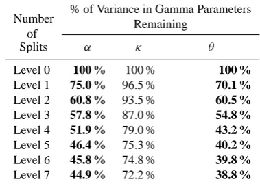
As before, the visual mapping of the connection between the catchment classes and the three parameters of the mixed gamma distribution was followed by a quantitative variabil-ity analysis; the result is summarized in Table 2. These results show that, with each step down the tree, the overall variabil-ity of all three parameters decreases, and thus these, like the dominant model processes, are explained by the classifica-tion tree in quantitative terms. However, not all parameters sort equally well; bothαandθshow significant reduction in variance whileκdoes not. This may be explained by the ba-sis for the classification scheme: the four criteria are mainly

Table 2. Variance reduction in parameters of the mixed gamma

dis-tribution sorted by catchment class.

Number % of Variance in Gamma Parameters

of Remaining

Splits α κ θ

Level 0 100 % 100 % 100 %

Level 1 75.0 % 96.5 % 70.1 %

Level 2 60.8 % 93.5 % 60.5 %

Level 3 57.8 % 87.0 % 54.8 %

Level 4 51.9 % 79.0 % 43.2 %

Level 5 46.4 % 75.3 % 40.2 %

Level 6 45.8 % 74.8 % 39.8 %

Level 7 44.9 % 72.2 % 38.8 %

Bold signifies a significant decrease in variance (p<1 %).

climate-oriented, as isα, and they utilize the RC, which re-flects the average values ofP andQover a long time pe-riod, as does θ. Where variance reduction is significant, it is greater in the first few splits on the tree than at the later branches. Forα, this is becauseαis nonzero when there is noP orQ; the larger theαis, the more intermittent the rain-fall or streamflow. The first two branchings of the tree imme-diately split off a large portion of humid catchments, where

α≈0 forQandQuand is small forP andQf, from the rest,

thus providing an immediate, and large, reduction in vari-ance. From the visual mapping, these same catchments also experienced very low seasonality and had very small ranges ofθ-values; thus splitting them off from their more variable counterparts provided immediate organization with respect toθ.

3.3 Dominant processes and the parameters of the mixed gamma distribution

The last part of the three-way mapping was the connection between the dominant model processes and the parameters of the mixed gamma distribution. Forα, the story is the same as outlined in the previous section. For the shape parameter, the process class “Vegetation” showed a wider variability of

κ-values relative to most of the other classes, notably large classes such as “Snow, Vegetation”, “Snow, SubQf,

Vegeta-tion”, and even “SubQf, Vegetation” (where “SubQf” refers

to subsurface-influencedQf)as seen in Fig. 7. Vegetation as

10−2 10−1 100 101

Base Model No Model Snow Snow, Sub Qf Snow, Sub Qf, Veg Snow, Veg Subsurf−influence QfSub Qf, Veg Vegetation

kappa

Q

Base No Snow Snow Snow Snow Subsurf Sub Qf Vegetation

Model Model Sub Q_f Sub Q_f Veg Q_f Veg Veg

Fig. 7. The parameterκ of the mixed gamma distribution for

to-tal streamflow grouped by dominant model process. Note that box width reflects number of catchments in each group.

as a wider range of κ-values. However, when snow and/or subsurface-influencedQf share dominance with vegetation,

the variability seems to be lessened. From our inspection of the shapes of the FDCs in Fig. 5, this seems to be borne out, at least for “Snow, SubQf, Vegetation” and “SubQf,

Vege-tation”, and may be caused by the presence of subsurface-influenceQf. We also saw from Ye et al. (2012) and

Coop-ersmith et al. (2012) that snow-dominated catchments share similar climate and physical properties; in addition, the pres-ence of snow in heavily vegetated areas further groups the catchments by climate and geology/topography, as the major-ity of these catchments are found in the northeastern US. This may explain in part the smaller variation inκ-values for cess classes containing snow and vegetation. However, pro-cess classes with snow but without vegetation contain many fewer catchments, and thus a more quantitative examination is necessary to determine if the smaller variability in theκ pa-rameter is significant. Forθ, the trend was not so clear, likely due to the wide range of climates (and therefore averageP

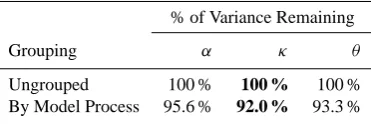
andQ)experienced within some model process classes. As shown in Fig. 7, some process classes contained fewer catchments than others, and so a visual assessment alone is insufficient to analyze differences between classes. Thus the connection between the dominant model processes and the three parameters of the mixed gamma distribution was ana-lyzed quantitatively using the variability analysis described in Sect. 2.2; the result is summarized in Table 3. As before, the results show a decrease in variance when the parameters are grouped compared to when they are not. Interestingly, when the parameters are grouped by dominant model pro-cess, the opposite is seen compared to when they are grouped by catchment class. Here κ shows statistically significant variance reduction whileαandθ do not; thus the shape pa-rameterκ is better described by the dominant model pro-cesses while both the scale parameterθandα, the fraction of

Table 3. Variance reduction in the parameters of the mixed gamma

distribution grouped by dominant model process.

% of Variance Remaining

Grouping α κ θ

Ungrouped 100 % 100 % 100 %

By Model Process 95.6 % 92.0 % 93.3 %

Bold signifies a significant decrease in variance (p<1 %).

no rainy or flow days, are better described by the catchment classification system. This may be because the classification system is based in large part on the climate – the amount and timing of water available to a catchment – while the domi-nant model processes are more closely related to catchment function, since they explicitly take into account the effect of interception, phenology, and subsurface-influencedQf.

3.4 Synthesis: the slope of the FDC

As was previously discussed, there is more than one way of quantifying the FDC: the fitted parameters of the mixed gamma distribution (α,κ,θ )or the slope of the FDC. How-ever, the three parameters describe the entire FDC, while the slope as defined here only describes the middle limb – the bridge between the high flows and the low flows. By focus-ing on one limb of the FDC at a time, more specific con-trols may be identified, since the analyses in previous sec-tions were not able to fully untangle the climate from the catchment controls. In this paper we only examine the slope of the middle limb of the FDC, as it is closely related to the RC, on which the modeling and classification studies were based; the upper and lower limbs are left for future work. The slopes of the FDC forQandQuwere grouped first by

class (Fig. 8) and then by dominant model process (Fig. 9). The box plots provide a visual assessment of the variability of the magnitudes of the slope of the FDC within each group-ing: the size of the box represents the 25th–75th percentile, while the whiskers show the minimum and maximum val-ues. Because of the way the slope is calculated, catchments with ephemeral streams or those for which the streamflow becomes very small at higher percent exceedance (i.e., drier catchments) will have very large slopes. This is clearly il-lustrated by the class XADB (high seasonality, arid, wetter winters) in Fig. 8, which consists entirely of arid catchments in southern California.

0 2 4 6 8 10 12 14

LBMH (1)

LBMS (3)

LJ (68)

LPC (11)

LPM (11)

LPQ (6)

LWC (21)

IACJ (3)

IAQ (6)

IHM (3)

ISCJ (5)

ISQJ (23)

ITC (19)

ITF (1)

IVD (1)

XACJ (2)

XADB (2)

XHD (2)

XSMB (1)

XTM (4)

XVM (3)

MIN

MEAN

MEDIAN MAX

Fig. 8. Total streamflow FDC slopes grouped by catchment class.

slopes than did those without (Fig. 9). However, from previ-ous examination (Fig. 7) we see that some of these process classes are quite small in size compared to others. Neverthe-less, when examining the four largest process classes aside from “Base Model” and “No Model”, the majority of the catchments in “Snow, SubQf, Vegetation” and “Snow,

Veg-etation” showed more narrow ranges of FDC slopes than did “SubQf, Vegetation” and “Vegetation”. These results mirror

those of the visual mapping done in previous sections, where low seasonality reduced variability in θ-values, and where snow processes reduced the variability inκ-values.

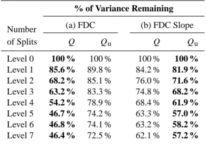
As with the three-way mapping, the visual assessment was followed by a variability analysis. Both the slope of the FDCs and the FDC quantiles were sorted on the catchment classi-fication decision tree. When the FDC quantiles were sorted along the tree, there was a monotonic decrease in variance for all duration curves, yet as before the most variance was explained in the first two levels. The result for theQFDC was significant (Table 4a), while that forQuwas not. When

the slopes of theQandQuFDCs were sorted along the tree,

the same pattern of early reduction of variance leveling off with further branching was repeated, but this time the slopes of theQuFDC showed a more significant reduction in

vari-ance than those of Q(Table 4b). The overall pattern seen here is similar to the reduction in variance obtained by sort-ing the gamma parameters on the classification tree; there too the decrease in variance (where significant) was greater in the early branchings than in the outer branches. This may again be explained in part by the way that the classifica-tion tree branches – the early splits remove a large porclassifica-tion of the low-seasonality, humid catchments from the distribu-tion, which (as visually mapped in Fig. 4c and d) have very similar FDCs, with the majority of the differences between the FDCs in each class seen at flows occurring>66 % of the time – i.e., the lower limb of the FDC.

Returning to the conceptual model presented in Sect. 1 of this paper, we have now analyzed the catchment response in-dicator, in the form of the FDC, from both the perspective of the entire FDC (parameters of mixed gamma distribution) and the middle limb of the FDC/regime curve (slope). What remains is to examine more closely the relationship between

0 2 4 6 8 10 12 14

Base Model No Model Snow Snow, Sub Qf

Snow, Sub Qf, Vegetation

Snow, Vegetation

Subsurface- Influenced

Qf Sub Qf, Vegetation

Vegetation MIN MEAN MEDIAN MAX

Fig. 9. Total streamflow FDC slopes grouped by dominant model

process.

Table 4. Variance reduction in FDC quantiles (a) and slopes (b)

sorted by catchment class.

% of Variance Remaining

Number (a) FDC (b) FDC Slope

of Splits Q Qu Q Qu

Level 0 100 % 100 % 100 % 100 %

Level 1 85.6 % 89.8 % 84.2 % 81.9 %

Level 2 68.2 % 85.1 % 76.0 % 71.6 %

Level 3 63.2 % 83.3 % 74.8 % 68.2 %

Level 4 54.2 % 78.9 % 68.4 % 61.9 %

Level 5 46.7 % 74.2 % 63.3 % 57.0 %

Level 6 46.8 % 74.1 % 63.2 % 58.2 %

Level 7 46.4 % 72.5 % 62.1 % 57.2 %

Bold signifies a significant decrease in variance (p<1 %).

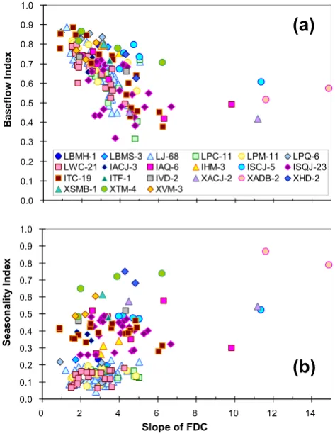
the FDC and the climate and catchment properties that define its shape. TheQFDC was plotted against both the season-ality index (SI), representing the climate, and the baseflow index (BI), representing the catchment (although we should note that climate factors into BI as well). As an additional layer of analysis, the slopes of the FDCs were grouped first by catchment class (Fig. 10) and then by dominant model process (Fig. 11) in order to determine if any clustering be-comes evident, which could help bring out which process governs which part of the FDC and could aid in regional-ization.

0.0 0.1 0.2 0.3 0.4 0.5 0.6 0.7 0.8 0.9 1.0

0 2 4 6 8 10 12 14

Basef

lo

w

I

n

d

ex

LBMH-1 LBMS-3 LJ-68 LPC-11 LPM-11 LPQ-6

LWC-21 IACJ-3 IAQ-6 IHM-3 ISCJ-5 ISQJ-23

ITC-19 ITF-1 IVD-2 XACJ-2 XADB-2 XHD-2

XSMB-1 XTM-4 XVM-3

0.0 0.1 0.2 0.3 0.4 0.5 0.6 0.7 0.8 0.9 1.0

0 2 4 6 8 10 12 14

Slope of FDC

S

ea

sona

lit

y Inde

x

(b)

(a)

Fig. 10. Relationship between baseflow index (a) and seasonality

index (b) and total streamflow FDC slopes (grouped by catchment class).

glance may seem at odds with the aridity of the region: one is dominated by vegetation processes, and the other by both snowmelt and vegetation processes. The first catchment is on the Caney River in Kansas, one of the Great Plains states, and closer inspection reveals a lush riparian corridor. Due to the aridity of the region, the stream may become dry in the summer months, thus causing the large FDC slope. In dry regions, phreatophytes may make up a large portion of the woody riparian vegetation. These deep-rooted plants, by tap-ping into shallow groundwater, draw down the water table; this can reduce streamflow, thus contributing in part to the steep slopes seen in these FDCs. The second catchment is on the Bad River in South Dakota, and is a snow-fed tributary of the Missouri River that flows in part through a national prairie grassland. The plot of the slope of theQuFDC (not

shown here for brevity) follows that for theQFDC, except shifted slightly to the left, as the slope of theQuFDC is

gen-erally less than that ofQ. This is likely due to the extreme high flows present in theQFDC pulling the curve upwards, thus steepening the overall slope.

0.0 0.1 0.2 0.3 0.4 0.5 0.6 0.7 0.8 0.9 1.0

0 2 4 6 8 10 12 14

Slope of FDC

S

ea

so

n

alit

y In

d

ex

0.0 0.1 0.2 0.3 0.4 0.5 0.6 0.7 0.8 0.9 1.0

0 2 4 6 8 10 12 14

B

asef

lo

w

I

n

d

ex

Base model No Model

Snow Snow, Sub Qf

Snow, Sub Qf, Vegetation Snow, Vegetation

Subsurface influenced Qf Sub Qf, Vegetation

Vegetation

(a)

(b)

Fig. 11. Relationship between baseflow index (a) and seasonality

index (b) and total streamflow FDC slopes (grouped by dominant model process).

4 Discussion

4.1 Comparative analysis: regionalization

a population of catchments. By examining the entire dataset across a population of catchments, we have identified regions of homogeneity, and have attempted to classify them in dif-ferent ways, as well as make connections between them in order to clarify how catchments behave in different locations, thus partitioning the nation into regions of similarity. By de-termining the underlying processes within a region, and in turn how they might vary by region, we gain understanding of the physical controls and in this way step closer to the ulti-mate goal, the prediction of the FDC, in any ungauged basin. The regional patterns highlighted in these four papers led to the groupings that have been explored both qualitatively and quantitatively in this synthesis analysis. We have shown that the variance within these groups, both in the three-way mapping and in the FDC slope analysis, was less than that between groups, thus objectively demonstrating that these groupings are meaningful. This is consistent with the idea that classification and catchment grouping is useful for es-timation of the FDC in ungauged catchments, particularly in large areas (see e.g., Sauquet and Catalogne, 2011). Of note is one region that was highlighted in all of our stud-ies, particularly the modeling and catchment classification: the Midwestern US. This is a mid-continent region of tran-sition to higher climate seasonality and aridity, and is also this country’s main agricultural region. While the MOPEX catchments are ostensibly minimally impacted by human be-havior (Duan et al., 2006), recent work by Wang and He-jazi (2011) has shown that this is not always the case. These human alterations have, in part, become dominant processes themselves, as illustrated by the simple model’s inability to perform satisfactorily in this part of the US, and thus must be taken into account in any regionalization studies with signif-icant anthropogenic activities.

The synthesis analysis of these groups showed that while the classification tree described well the scale parameterθ, and the zero exceedance parameterα, the dominant model processes better described the shape parameterκ. Since the model processes focus more on catchment function, this gives first-order physical meaning to the shape parameter. However, there was no unique value of κ for each model process, which points to the need for a more complex model than we use here, such as the process-based model of Car-illo et al. (2011) and others like it that can capture catchment properties in greater detail and thus bring out their controls on the FDC. Since the climate and catchment function are so closely linked through geologic time by co-evolution, more specific properties of the catchment, such as topography, soil types, etc., all of which determine in part the filtering of infil-trated precipitation and thus the FDC at the outlet, may need to be included. Thus, with the catchment more explicitly de-fined in the model, the effects of the catchment itself may be separated from the effects of the climate it experiences. In addition, the parameter fitting itself was strongly affected by the tails of the FDC. Parameter values containing more

close fits to the tails would likely produce stronger synthesis relationships with the model processes.

Further analysis into the slope of theQFDC revealed that the baseflow index was a stronger control on it than was the seasonality index. The slope of the FDC as defined here is re-lated to the RC, which is a function of long-term catchment response, and this would confirm the idea that the middle limb of the FDC is related to the RC. Clustering of classes and model processes was seen in the scatter plots (Figs. 10 and 11); catchments in the region where snowmelt is the dominant process tended to all have higher BI, while the veg-etation process dominated regions explored a larger range of BI. Combining the results of this study and the empirical one, we see that catchments with largerκ-values tended to also have larger BI (a greater proportion ofQexits as Qu)

and flatterQandQuFDC slopes. These results seem to

in-dicate that catchment properties rather than the more time-dependent climate properties are the dominant controls on the FDC. Climate seasonality does affect the catchment re-sponse as the classification study highlighted, and to some extent the shape of the FDC, as the empirical study high-lighted, but the control is secondary to the catchment proper-ties, as evidenced by the stronger relationship of the slope of the FDC to BI compared to SI, and the more significant vari-ance reduction of theQuFDC compared to theQFDC when

sorted on the classification tree. Seasonality implies timing; the FDC removes the time element, and by doing so may also provide a first-order separation of climate influence from that of catchment properties.

That the relationship is stronger with BI may be due to the way the slope of the FDC is calculated. A slope obtained using Eq. (2) represents the middle limb of the FDC, which itself represents the long-term, averaged response from the catchment. Since the baseflow index also is a measure of these processes, and as such is governed more by the to-pography and other earth processes than by climate pro-cesses, this result confirms the hypothesis of Yokoo and Siva-palan (2011) that the middle limb of the FDC is a function of the RC. This relationship of the shape of the FDC with groundwater-related measures has also been seen previously in the literature, in studies not limited to the US. For example, Claps and Fiorentino (1997) use BI to regionalize the FDC in Basilicata, in southern Italy. Similarly, in the UK the HOST classification of soils is used as a surrogate for the geology (Holmes et al., 2002). Sauquet and Catalogne (2011) found that the catchment yield and the percentage of impermeable substratum (which are more or less related to the geology) are among the most important explanatory variables to re-gionalize the FDC in France.

for in other works. For example, in Arora et al. (2005) and Ganora et al. (2009) the mean catchment elevation is used to discriminate between regions with different FDCs in Nepal and Italy respectively, and it is argued that elevation is a proxy for distinguishing areas more or less influenced by snow mechanisms (and therefore different seasonality). Li et al. (2010) found that the leaf area index is correlated to the shape of the FDC in south-eastern Australia; vegetation im-pacts ET differentially between summer and winter, increas-ing the slope of the FDC and the probability of havincreas-ing zero flow for some portion of the year, similar to what was seen in some of the more arid regions in the US. These implicit sea-sonality effects were also seen in the MOPEX catchments when vegetation-related dominant model processes led to higher variability and steeper slopes in the FDC. Thus the findings of this study, based solely on catchments in the con-tinental US, correlate with findings from a more global per-spective and further highlight this co-evolutionary relation-ship between climate and catchment properties.

4.2 Comparative analysis: regime curve and the flow duration curve

The aim of this study was to determine the underlying phys-ical controls on the FDC. However, another, less expected, theme that kept surfacing throughout the entire study was that the differences between catchment responses are more readily seen in the RC than in the FDC. These differences between catchments appear more obviously, and the reasons for those differences are far more straightforward, in the RC in part because the temporal pattern remains intact, while in the FDC this information is removed. From both the catch-ment classification study (Coopersmith et al., 2012) and the process modeling study (Ye et al., 2012), it was shown that many of the processes controlling the catchment response are time-dependent, for example, the seasonality of precipitation or the vegetation processes of tree leaf-out and leaf-drop. In addition, it is not uncommon for more than one hydrologic control process to be at work in a given catchment; thus one complicating factor in relating the regional patterns seen in these studies to the physical controls on the FDC is that the patterns obtained for both the dominant model processes and the classification system were based on the RC, not the FDC. The guiding principle behind these two studies was that the RC and middle limb of the FDC are related to each other, and we have seen evidence of this in both this paper and in the sta-tistical study (Cheng et al., 2012). To further understand this relationship between the RC and the FDC, we have again ap-proached it both qualitatively, by examining RCs and FDCs from a few selected catchments in the study, and quantita-tively, by comparing the slopes of both the FDC and the RC plotted as an FDC.

Qualitatively, the information about process controls on the catchment response contained within the FDC is more subtle, since removal of the time element filters out what

this work has shown to be crucial information. This might lead one to think that two catchments with different regime curves could have the same FDC. However, as Fig. 12 shows, this is not always true; there is still some information to be gained from the FDC. For the catchment in Montana (MT), when looking at the RC, the peak in streamflow caused by snowmelt is quite prominent, but, for the rest of the year,Q

is relatively constant. This can be seen in the FDC of MT as a fairly flat slope through most of the curve, with a slight uptick at the rarely exceeded (high flows) end, as in this catchment the highest flows generally correspond to the an-nual snowmelt events. Contrast this with the semi-arid catch-ment in Kansas (KS), where the streamflow varies a great deal throughout the year. This is seen in the FDC of KS as a much steeper slope overall, with the aridity of the catchment indicated by the curve tending to zero flow before 100 % ex-ceedance. Thus catchments with very different RCs also have different FDCs, although this difference is much less pro-nounced. Catchments with very similar RCs have even more similar FDCs, as illustrated by the two forested catchments in Pennsylvania (PA) and Virginia (VA); here the seasonal pat-terns of leaf-out in the spring and leaf-drop in the fall are seen in the RC as a decrease in streamflow from about May to Oc-tober, even though the precipitation for the east coast of the US is fairly constant all year. This phenology signature is less clear in the FDC, where the two catchments are nearly indis-tinguishable from one another – except at the extreme ends – and not substantially different from the MT catchment de-scribed earlier. In spite of this, some differences in the shape of the FDCs can be related to possible physical controls, the arid catchment in Kansas being a good example of this. Note that the major differences in these example FDCs are in the tails; this is where the story of the FDC may lie, and it is pos-sible that an analysis of extremes may illuminate this further. Also, this example only highlighted theQFDC; it may also be that the FDCs of the componentsQfandQu, as well as

their tails, may further elucidate the physical controls on the FDC.

1 31 61 91 121 151 181 211 241 271 301 331 361 0

1 2 3 4

Julian Day Smoothed daily Q (mm) / Mean annual daily Q (mm)

PA, LJ, Snow, Sub Qf, Vegetation MT, LPQ, Snow

North CA, XHD, Subsurface−influenced Q_f KS, ISQJ, Vegetation

VA, LJ, Snow

0 10 20 30 40 50 60 70 80 90 100

10−3 10−2 10−1 100 101 102

Probability of Exceedance

Daily Q (mm) /

Mean annual daily Q (mm)

PA, LJ, Snow, Sub Qf, Vegetation MT, LPQ, Snow

North CA, XHD, Subsurface−influenced Qf

KS, ISQJ, Vegetation VA, LJ, Snow

Fig. 12. Smoothed regime curve of total streamflow (top) and

cor-responding flow duration curve (bottom), both at the daily scale and normalized by mean annual daily flow. (Legend description is given as US state abbrev., catchment class, dominant model process).

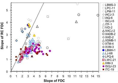
slope of an RC FDC is much lower than the corresponding FDC middle limb. By grouping these slopes by catchment classes, we see some interesting regional patterns emerge. The catchments where the RC FDC slope is the same or larger than the corresponding FDC cluster mainly in the low-to-mid seasonality, more humid catchments in the northwest central US (e.g., LBMH, LPQ, IHM). This region is domi-nated by snowmelt processes, as illustrated by the MT catch-ment shown in Fig. 12, and this is seen quantitatively in both the RC and the FDC through their slopes. Catchments in the low-seasonality, humid east coast (e.g., classes LJ and LWC) tended to have RC FDC slopes closer to those of their cor-responding FDC than did the intermediate-seasonality catch-ments in the mid-continent region (e.g., ISQJ and ITC). In the eastern, deciduous-forested catchments, the spring flow peak followed by the sharp decline in streamflow during the sum-mer months (as illustrated by the PA catchment in Fig. 12) serves to mimic the extremes seen in the FDC tails, thus steepening the RC FDC somewhat. This, combined with the flatter overall slope of FDCs in humid regions, brings the RC FDC slope closer to the slope of the corresponding FDC. However, this clear spring peak/summer low flow regime be-havior is generally not seen in the RCs of catchments in the Midwest, which are dominated by grassland and more sea-sonal precipitation. Because the averaging processes inher-ent in producing a regime curve further smooth out the dif-ferences between the extreme flows, RC FDC slopes from catchments in this region deviate even further from their cor-responding FDC slope.

0 1 2 3 4 5

0 1 2 3 4 5 6 7 8 9 10 11 12 13 14 15

Slope of FDC

S

lope

of

R

C

FD

C

LBMS-3 LPC-11 LPM-11 IACJ-3 IAQ-6 ISCJ-5 ITF-1 IVD-2 XACJ-2 XADB-2 XHD-2 XSMB-1 XTM-4 XVM-3 LBMH-1 LJ-68 LPQ-6 LWC-21 IHM-3 ISQJ-23 ITC-19

Fig. 13. Relationship between the slope of the FDC and the slope

of the RC when plotted as an FDC (grouped by catchment class). A 1 : 1 line is provided for reference.

5 Conclusions

The visual mapping done here showed that, within each regime class, both process and empirical, there was a great deal of heterogeneity in the shapes of the FDC, which was most noticeable in the tails. This emphasized a finding of the first study, where the statistical fitting was strongly affected by the tails of the FDC. While the upper tail is most affected by the precipitation intensity, the lower tail is affected more by catchment properties of landscape, soils, geology, etc. than by climate. Thus further analysis of the tails of the FDC, especially the low flows, may separate the physical controls on the shape of the FDC more effectively. In moving for-ward, the modeling study must also be enhanced to incorpo-rate these high and low flow processes. The similar regions delineated in this study, based on the regime curve, can be used to “zoom in” on a particular class, guiding the appli-cation or development of more detailed models to bring out the differences in the underlying physical (as well as anthro-pogenic) controls at work in each region. Under this frame-work, the coupled soil-water-plant growth analytical model of Feng et al. (2012) and the detailed process-based model of Carillo et al. (2011) are the kind of models that would be better suited to fully separate the catchment controls of the FDC from the climate controls. We leave the pursuit of this exploration to future research.

Acknowledgements. The work presented in this paper was carried out as part of the NSF-funded project “Water Cycle Dynamics in a Changing Environment: Advancing Hydrologic Science through Synthesis” (NSF grant EAR-0636043, M. Sivapalan, PI), also the NSF project “Understanding the Hydrologic Implications of Land-scape Structure and Climate – Toward a Unifying Framework of Watershed Similarity” (NSF Grant EAR-0635998, T. Wagener, PI). Special thanks are owed to Matej Durcik of SAHRA (University of Arizona) for providing the version of the MOPEX dataset used in this study. We also wish to thank our referees for their constructive criticism and insights which have helped us improve this work.

Edited by: A. Castellarin

References

Arora, M., Goel, N. K., Singh, P., and Singh, R. D.: Regional flow duration curve for a Himalayan river Chenab, Nord. Hydrol., 36, 193–206, 2005.

Botter, G., Porporato, A., Rodriguez-Iturbe, I., and Rinaldo, A.: Basin-scale soil moisture dynamics and the probabilistic char-acterization of carrier hydrologic flows: Slow, leaching-prone components of the hydrologic response, Water Resour. Res., 43, W02417, doi:10.1029/2006WR005043, 2007a.

Botter, G., Porporato, A., Daly, E., Rodriguez-Iturbe, I., and Ri-naldo, A.: Probabilistic characterization of base flows in river basins: Roles of soil, vegetation, and geomorphology, Water Re-sour. Res., 43, W06404, doi:10.1029/2006WR005397, 2007b. Botter, G., Zanardo, S., Porporato, A., Rodriguez-Iturbe, I.,

and Rinaldo, A.: Ecohydrological model of flow duration

curves and annual minima, Water Resour. Res., 44, W08418, doi:10.1029/2008WR006814, 2008.

Botter, G., Porporato, A., Rodriguez-Iturbe, I., and Rinaldo, A.: Nonlinear storage-discharge relations and catchment streamflow regimes, Water Resour. Res., 45, W10427, doi:10.1029/2008WR007658, 2009.

Breiman, L., Friedman, J., Olshen, R., and Stone, C.: Classification and Regression Trees, Chapman and Hall, Boca Raton, 1993. Brooks, P. D., Troch P. A., Durcik, M., Gallo, E., and Schlegel,

M.: Quantifying regional-scale ecosystem response to changes in precipitation: Not all rain is created equal, Water Resour. Res., 47, W00J08, doi:10.1029/2010WR009762, 2011.

Carrillo, G., Troch, P. A., Sivapalan, M., Wagener, T., Harman, C., and Sawicz, K.: Catchment classification: hydrological analysis of catchment behavior through process-based modeling along a climate gradient, Hydrol. Earth Syst. Sci., 15, 3411–3430, doi:10.5194/hess-15-3411-2011, 2011.

Castellarin, A., Vogel, R. M., and Brath, A.: A stochastic index flow model of flow duration curves, Water Resour Res., 40, W03104, doi:10.1029/2003WR002524, 2004.

Castellarin, A., Camorani, G., and Brath, A.: Predicting annual and long-term flow-duration curves in ungauged basins, Adv. Water Resour., 30, 937–953, 2007.

Cheng, L., Yaeger, M., Viglione, A., Coopersmith, E., Ye, S., and Sivapalan, M.: Exploring the physical controls of re-gional patterns of flow duration curves – Part 1: Insights from statistical analyses, Hydrol. Earth Syst. Sci., 16, 4435–4446, doi:10.5194/hess-16-4435-2012, 2012.

Claps, P. and Fiorentino, M.: Probabilistic flow duration curves for use in environmental planning and management, in: Integrated Approach to Environmental Data Management Systems, edited by: Harmancioglu, N. B., Alpaslan, M. N., Ozkul, S. D., and Singh, V. P., Kluwer Academy, NATO ASI Series, 2, 255–266, 1997.

Coopersmith, E., Yaeger, M. A., Ye, S., Cheng, L., and Sivapalan, M.: Exploring the physical controls of regional patterns of flow duration curves – Part 3: A catchment classification system based on regime curve indicators, Hydrol. Earth Syst. Sci., 16, 4467– 4482, doi:10.5194/hess-16-4467-2012, 2012.

Duan, Q., Schaake, J., Andr´eassian, V., Franks, S., Goteti, G., Gupta, H. V., Gusev, Y. M., Habets, F., Hall, A., Hay, L., Hogue, T., Huang, M., Leavesley, G., Liang, X., Nasonova, O. N., Noil-han, J., Oudin, L., Sorooshian, S., Wagener, T., and Wood, E. F.: Model Parameter Estimation Experiment (MOPEX): An overview of science strategy and major results from the second and third workshops, J. Hydrol., 320, 3–17, 2006.

Feng, X., Vico, G., and Porporato, A.: On the effects of seasonality on soil water balance and plant growth, Water Resour. Res., 48, W05543, doi:10.1029/2011WR011263, 2012.

Ganora, D., Claps, P., Laio, F., and Viglione, A.: An approach to estimate nonparametric flow duration curves in ungauged basins, Water Resour. Res., 45, W10418, doi:10.1029/2008WR007472, 2009.

Holmes, M. G. R., Young, A. R., Gustard, A., and Grew, R.: A re-gion of influence approach to predicting flow duration curves within ungauged catchments, Hydrol. Earth Syst. Sci., 6, 721– 731, doi:10.5194/hess-6-721-2002, 2002.

Li, M., Shao, Q., Zhang, L., and Chiew, F. H. S.: A new re-gionalization approach and its application to predict flow du-ration curve in ungauged basins, J. Hydrol., 389, 137–145, doi:10.1016/j.jhydrol.2010.05.039, 2010.

L’vovich, M. I.: World Water Resources and Their Future, translated from Russian by Nace, R. L., 415 pp., AGU, Washington, DC, 1979.

Muneepeerakul, R., Azaele, S., Botter, G., Rinaldo, A., and Rodriguez-Iturbe, I.: Daily streamflow analysis based on a two scaled gamma pulse model, Water Resour. Res., 46, W11546, doi:10.1029/2010WR009286, 2010.

Sauquet, E. and Catalogne, C.: Comparison of catchment group-ing methods for flow duration curve estimation at ungauged sites in France, Hydrol. Earth Syst. Sci., 15, 2421–2435, doi:10.5194/hess-15-2421-2011, 2011.

Sawicz, K., Wagener, T., Sivapalan, M., Troch, P. A., and Carrillo, G.: Catchment classification: empirical analysis of hydrologic similarity based on catchment function in the eastern USA, Hy-drol. Earth Syst. Sci., 15, 2895–2911, doi:10.5194/hess-15-2895-2011, 2011.

Sivapalan, M., Thompson, S. E., Harman, C. J., Basu, N. B., and Kumar, P.: Water cycle dynamics in a changing environment: Im-proving predictability through synthesis, Water Resour. Res., 47, W00J01, doi:10.1029/2011WR011377, 2011a.

Sivapalan, M., Yaeger, M. A., Harman, C. J., Xu, X., and Troch, P. A.: Functional model of water balance variability at the catchment scale: 1. Evidence of hydrologic similarity and space-time symmetry, Water Resour. Res., 47, W02522, doi:10.1029/2010WR009568, 2011b.

Vogel, R. M. and Fennessey, N. M.: Flow-duration. I: New interpre-tation and confidence intervals, J. Water Resour. Pl.-ASCE, 120, 485–504, 1994.

Vogel, R. M. and Fennessey, N. M.: Flow duration curves II. A re-view of application in water- resources planning, Water Resour. Bull., 31, 1029–1039, 1995.

Walsh, P. D. and Lawler, D. M.: Rainfall seasonality: description, spatial patterns and change through time, Weather, 36, 201–208, 1981.

Wang, D. and Hejazi, M.: Quantifying the relative contribution of the climate and direct human impacts on mean annual streamflow in the contiguous United States, Water Resour. Res., 47, W00J12, doi:10.1029/2010WR010283, 2011.

Yadav, M., Wagener, T., and Gupta, H.: Regionalization of con-straints on expected watershed response, Adv. Water Resour., 30, 1756–1774, 2007.

Ye, S., Yaeger, M., Coopersmith, E., Cheng, L., and Sivapalan, M.: Exploring the physical controls of regional patterns of flow du-ration curves – Part 2: Role of seasonality, the regime curve, and associated process controls, Hydrol. Earth Syst. Sci., 16, 4447– 4465, doi:10.5194/hess-16-4447-2012, 2012.