Short term power load forecasting using Deep Neural Networks

Short Term Power Load Forecasting

Using Deep Neural Networks

Ghulam Mohi Ud Din Department of Computer Science Liverpool John Moores University

United Kingdom [email protected]

Angelos K. Marnerides

Infolab21, School of Computing & Communications Lancaster University

United Kingdom

[email protected]

Abstract—Accurate load forecasting greatly influences the planning processes undertaken in operation centres of energy providers that relate to the actual electricity generation, distribu-tion, system maintenance as well as electricity pricing. This paper exploits the applicability of and compares the performance of the Feed-forward Deep Neural Network (FF-DNN) and Recurrent Deep Neural Network (R-DNN) models on the basis of accuracy and computational performance in the context of time-wise short term forecast of electricity load. The herein proposed method is evaluated over real datasets gathered in a period of 4 years and provides forecasts on the basis of days and weeks ahead. The contribution behind this work lies with the utilisation of a time-frequency (TF) feature selection procedure from the actual ”raw” dataset that aids the regression procedure initiated by the aforementioned DNNs. We show that the introduced scheme may adequately learn hidden patterns and accurately determine the short-term load consumption forecast by utilising a range of heterogeneous sources of input that relate not necessarily with the measurement of load itself but also with other parameters such as the effects of weather, time, holidays, lagged electricity load and its distribution over the period. Overall, our generated outcomes reveal that the synergistic use of TF feature analysis with DNNs enables to obtain higher accuracy by capturing dominant factors that affect electricity consumption patterns and can surely contribute significantly in next generation power systems and the recently introduced SmartGrid.

Index Terms—Short Term Load Forecasting, Feed-forward Deep Neural Network, Recurrent Deep Neural Network, Time-Frequency Analysis.

I. INTRODUCTION

Power load forecasting holds a crucial role in the ca-pacity planning process of power systems scheduling and maintenance as well as end-consumer awareness regarding viewing timely their consumption behaviour and bills. The actual forecasting of the power load distribution is classified into short, medium and long term forecasting. Short term load forecasting (STLF) is associated with load prediction from few hours to few days ahead whereas medium term load forecasting (MTLF) deals with forecasts targeting few weeks to few months ahead. On the other hand, long term load forecasting (LTLF) deals with load prediction from one year to several years. LTLF assists in planning of new power systems setup, MTLF aids in system maintenance, purchasing energy and pricing plans whereas STLF plays a key role in unit commitment, power distribution and load dispatching. STLF is a challenging task due to short time duration as it requires

instant and accurate decisions. The errors in STLF can have either leptokurtic or the normal distribution. If the normal distribution is assumed, it represents the tail of distribution insufficiently and leads to under-committing power systems which can cause shortage of energy in market and eventually increases the cost to produce more energy [1].

A number of studies have developed different methods to accurately forecast electricity load in recent years. Traditional statistical load forecasting methods are inadequate to fully model the complex nature of electricity demand and often result in lower accuracy [2]. Artificial Intelligence (AI) based techniques are most favourable due to their ability to tackle non-linear relationships between dependent and independent variables. Fuzzy logic [3], artificial neural networks [4], sup-port vector machines [5] and wavelets neural networks [6] are popular AI techniques for STLF. Due to the state-of-the-art success of deep neural network methods in image processing, they are naturally being adapted for general time series modelling tasks such as those for load forecasting. Busseti et al. [7] predicted load demands by utilizing only time and temperature data by performing prediction using deep neural and recurrent neural networks. In fact, the outcomes behind the aforementioned study achieved an RMSE error of 530 KW/h using a three layer recurrent neural network. Khan et al. [8] proposed a recurrent neural network model for half an hour ahead load forecasting whereas Agarwal et al. [6] developed ANN models for hour ahead load and price forecasts using the load data from ISO New England1_{) that} we also use in this paper.

In this work, Feed-froward Deep Neural Networks (FF-DNN) and Recurrent Deep Neural Networks (R-(FF-DNN) based models are presented to predict short term electricity load. Achieving higher accuracy in forecasts requires to include all the related factors that affect the overall electricity con-sumption. This is accomplished by initially analysing the data on the time and frequency domain independently and subsequently frequency domain components are transformed back to the time domain. The resulted time-frequency (TF) features efficiently capture dominant effects i.e. weather, time,

working and non-working days, lagged load and data distri-bution effects. Due to the constantly changing environment, electricity consumption patterns of domestic as well as com-mercial users carry complex characteristics. These characteris-tics are analyzed in time and frequency domain and prediction performance of deep networks is compared on the basis of RMSE, MAE and MAPE error measures. The results obtained with the developed methodology indicate least MAPE errors as compared to other existing models (e.g., [9]).

The remaining sections are organized as follows. In section II, the description and pre-processing of the dataset in time and frequency domain is given. Section III is dedicated for the description of the FF-DNN and R-DNN-based models whereas section IV presents the methodology that covers data pre-processing as well as the aspects of data training and prediction models. Section V exhibits the analysis and results obtained from our experimentation. Finally work is concluded in section VI.

II. DATADESCRIPTION ANDPRE-PROCESSING The electricity load dataset is collected from ISO New England (ISO-NE) for the duration 2007 to 2012. The load consumption values are recorded at the end of each hour in a day. The whole dataset consists of 52600 records and that represents the load for 6 states in New England, USA. Table I depicts the original features in the dataset and their description.

TABLE I

ORIGINALFEATURES INDATASET

Feature Description Date Date (MM/DD/YYY)

Hour Hour of the day (24 Load values in a day) ElecPrice Price of the electricity (MW/h)

DryBulb Dry bulb temperature (Fahrenheit) DewPnt Dew point temperature (Fahrenheit) SYSLoad NEPOOL system load = [generation

- pumping load + net interchange] as determined by metering (MWh)

A. Extracting Features from Original Dataset

The original dataset contains features that do not properly accentuate the effect of various factors and results to the elec-tricity consumption profiles of users highly to be statistically non-linear and complex. Our empirical observations led to consider factors such as weather, time, holidays, lagged load and load distribution in different time periods to be the most influential to electricity consumption on a daily basis.

1) Time Domain Feature Extraction: The original dataset is analysed in time domain to capture the changing behaviour of electricity consumption patterns with respect to time. The following effects are captured using time domain analysis of data.

Temperature Effects

Fig. 1 highlights that daily consumption of electricity over the week is affected by temperature. When the temperature is higher during the day time, more electricity is consumed to

make temperature suitable according to the environment. Dry bulb and dew points are used to determine the humidity in the air. Different amount of electricity is consumed to maintain the humidity in summer and winter seasons. Dry bulb and Dew point features has been selected to represent temperature effect on the electricity consumption.

Fig. 1. Variations in Temperature and Load for 1 Week

Working and Non-Working Days Effects

In fig. 1 from Monday to Friday, electricity consumption is high while on Saturday and Sunday electricity consumption is low. Based on these observations the ”Is Working Day feature” is selected to express this effect.

Time Effect

Fig. 1 also suggests that the electricity consumption is highly dependent over time. Electricity consumption values represent ascending and descending effect before and after the midday respectively. Two feature are derived to the express the time dependency as Hour and the Week Day.

Lagged Load Effect

Lagged hourly peak load values contain vital information about specific patterns of users’ electricity consumption. This information can be extracted using multiple lagged load values with the features Prev. Day Same Hour load, Prev. 24 Hours Average Load and Prev. Week Same Hour Load.

Data Distribution Effect

The data distribution effects are captured over the past 24 hours using skewness, kurtosis, variance and periodicity. These features uncover hidden patterns in the dataset efficiently and assist neural networks to provide highest load prediction accuracy.

stable and easily predictable that considerably improves the accuracy. Fast Fourier analysis is performed on the electricity load values to determine dominant frequencies. The following equation converts load values into unnormalized univariate discrete Fourier transformed sequence.

y(k) =

N_X1

n=0

x(n)e i2⇡kn/N

Where x(n)represents time domain signal (n= 0...N 1), y(k) depicts transformed signal in frequency domain (k =

0...N 1) and N is the length of the input signal. Fig. 2

represents Fourier coefficients extracted from the electricity load values.

0e+00 2e+07 4e+07 6e+07

0 10000 20000 30000 40000

freqindex

Mod(coef)

Fig. 2. Fourier coefficients of electricity load

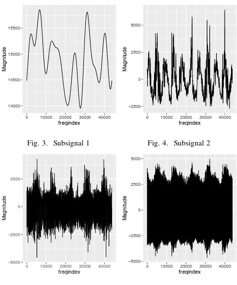
The Fourier coefficients with higher magnitude represent dominant frequencies. A high pass filter is designed to filter these dominant frequencies from low frequencies. The filtered signals are converted back to time domain. Figs. 3-6 highlight the filtered signals obtained from frequency domain analysis. III. DEEPNEURALNETWORKS FORSHORTTERMLOAD

FORECASTING

Neural networks try to replicate human brain functionality and possess the capabilities to learn hidden non-linear and complex structures in the data. Hinton et al. [10] proposed Deep Belief Network (DBN) and showed that deep archi-tectures can be trained using greedy layer wise pre training techniques. In this work, two models based on FF-DNN and R-DNN, are proposed for day and week ahead short term load forecasting.

A. Feed-forward Deep Neural Network (FF-DNN)

A neuron is the basic unit of FF-DNN model, structurely inspired by the human neuron. In FF-DNN model, the input

x is combined with weight w and biasbat the neuron using

following equation.

=

N_X1

n=0

wnxn+b

A nonlinear activation function is applied on computed which produces an output and sends as input to other con-nected neurons. The basic goal of FF-DNN is to approximate the function ( ).

14000 14500 15000 15500

0 10000 20000 30000 40000

freqindex

Magnitude

Fig. 3. Subsignal 1

−2500 0 2500 5000

0 10000 20000 30000 40000

freqindex

Magnitude

Fig. 4. Subsignal 2

−5000

−2500 0 2500

0 10000 20000 30000 40000 freqindex

Magnitude

Fig. 5. Subsignal 3

−5000

−2500 0 2500 5000

0 10000 20000 30000 40000

freqindex

Magnitude

Fig. 6. Subsignal 4

Multi-layer Feed-forward Neural Networks are made up of many such neurons interconnected in different layers. The output of the model is fully decided by weights and biases. The network learns by adjusting weights to minimize loss function with the large set of training data. The loss function is given by

Loss(q|W, B)

Where q represents each training example in the data, W is

the matrix of weights and B is the set of biases.

B. Recurrent Deep Neural Network (R-DNN)

The Multi-layer perceptron is the simplest form of R-DNN in which output of one hidden layer along with the input is fed back in the network. The following non-linear equations delineate the functionality of simple structure of R-DNN.

Q(t) =f1(X(t)⇤Wi+Q(t 1)⇤Wtd)

Y(t) =f2(Q(t)⇤Wi)

Where X(t) is input at time t, Q(t) is output, Q(t 1) is

IV. METHODOLOGY

In the proposed methodology, the first step is to extract features which comprehensively model all the factors affecting electricity consumption. To achieve this, the dataset is analysed in both time and frequency domain. The temperate, time, holidays, lagged load and data distribution effects are found to be the dominant factors affecting load. The second step is the selection of optimal model parameters.

First we show the parameter selection for FF-DNN model. We employ Rectifier activation function (ReLU) in the model because it is biologically accurate and shows high performance in image processing. It is defined as

f(x) =max(0, x) where f(x)2R

ReLU takes less processing time as it works on un-normalized data. As compared to Sigmoid or Tanh, exponential com-putation is not required in ReLU. Further, ReLU does not suffer from vanishing gradient problem. Although standard stochastic gradient efficiently utilises memory, but it becomes slow and requires memory locking and synchronization. We solve this issue by using newly developed lock free technique called Hogwild. This technique uses shared memory model and update loss function asynchronously. To include the effects of all factors in the model, time and frequency domain analysis suggests to use more features. This improves the prediction accuracy but at the cost of complexity. This makes the model complex which causes the problem of over-fitting. This problem is addressed using regularization techniques. We employL1(Lesso) regularization which adds an extra term in

the loss function to minimize error.

Loss0(q|W, B) =Loss(q|W, B) + (q|W, B)

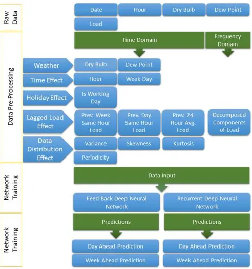
Where is a regularized term and it is selected using cross-validation. Fig. 7 visually describes the methodology of whole process i.e. data pre-processing, extracted features, training and prediction using FF-DNN and R-DNN.

V. ANALYSIS ANDRESULTS

In this section, we evaluate our proposed FF-DNN and R-DNN models for different seasons in 2012 and we use training data covering the years 2007 up to 2011. The Training dataset contains 43824 records while test dataset contains 24 and 168 records for day and week ahead forecasting respectively. The new features extracted from the original 5 features increase the accuracy of the models. For the evaluation of the models, RMSE, MAE and MAPE have been calculated for each forecasting type in four seasons of 2012 which are summarized in table 2. As we explain next, the predictions are made on the basis of two case studies.

Case Study I

In case study I, we use only time domain features and make predictions for day and week ahead using both FF-DNN and R-DNN models. Due to temperature variations in different seasons, electricity consumption varies considerably and we forecast load in winter, spring, summer and autumn separately.

Fig. 7. Visual Description of Load Prediction Methodology

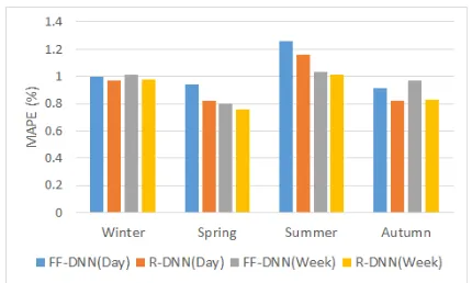
The time domain MAPE, RMSE and MAE errors are shown in table 2 for FF-DNN and R-DNN. The proposed models are able to get least MAPE, RMSE and MAE errors in spring season while highest errors are found in summer season as depicted in fig. 8. This is due to the unexpected variations in electricity consumption because of high temperature and social events in summer season.

A. Case Study II

In case study II, we use composite features from time and frequency domain analysis and forecast day and week ahead electricity load using FF-DNN and R-DNN. The errors are listed under frequency domain column in table 2 for both models. The accuracy is improved and the errors are much lower as compared to the errors found in case study I.

VI. CONCLUSION

TABLE II

SUMMARY OF THE PREDICTION ERRORS USINGTIME ANDFREQUENCY DOMAIN FEATURES WITHFF-DNNANDR-DNNMODELS

Season Forecast_Type MAPE(%) RMSE(MW/h) MAE(MW/h)

Time Domain Frequency Domain Time Domain Frequency Domain Time Domain Frequency Domain

FF-DNN DNNR- DNNFF- DNNR- ModelOther DNNFF- DNNR- DNNFF- DNNR- DNNFF- DNNR- DNNFF- DNN

R-Winter Day 1.00 0.97 0.019 0.016 2.47 202 194 3.84 3.55 152 141 2.81 2.63

Week 1.01 0.98 0.035 0.029 1.21 188 178 6.19 5.73 149 138 4.98 4.54

Spring Day 0.94 0.82 0.030 0.023 0.36 159 144 4.78 4.35 139 124 4.40 4.21

Week 0.80 0.76 0.026 0.020 0.54 135 126 4.27 4.02 104 95 3.35 3.10

Summer Day 1.26 1.16 0.060 0.045 209 202 11.86 9.06 103 98 10.67 9.60

Week 1.03 1.01 0.078 0.056 284 366 16.52 15.33 292 277 13.47 11.97

Autumn Day 0.91 0.82 0.036 0.026 190 175 6.36 5.86 133 116 5.00 4.42

Week 0.97 0.83 0.039 0.029 179 162 7.28 6.33 131 118 5.14 4.81

Whole

Year Year 1.42 1.30 0.067 0.057 1.29 306 287 131 119 210 197 6.99 5.96

In parallel, we exhibit the superiority of utilising TF features by comparison over a scenario where strictly time domain features are used with respect to forecasting statistical errors using three distinct error measures. Thus, we show the impor-tance of the initial employment of TF-based feature selection over bulk power measurements in order to improve the level of statistical forecasting accuracy. Overall, we argue the the approach proposed in this work may significantly contribute towards the accurate forecasting that is considered as a critical necessity in today’s power distribution operation centres.

Fig. 8. MAPE error comparison using Time domain features

ACKNOWLEDGMENTS

The authors would like to thank the UK EPSRC funded ”Situation Aware Information Infrastructure” (SAI2_{) project,}

EP/L026015/1, that has kindly supported this work. REFERENCES

[1] B. M. Hodge, D. Lew, and M. Milligan, “Short-term load forecast error distributions and implications for renewable integration studies,”IEEE Green Technologies Conference, pp. 435–442, 2013.

[2] F. Marin, F. Garcia-Lagos, G. Joya, and F. Sandoval, “Global model for short-term load forecasting using artificial neural networks,”IEE Proceedings - Generation, Transmission and Distribution, vol. 149, no. 2, p. 121, 2002.

Fig. 9. MAPE error comparison using Time and frequency domain features [3] A. Badri, Z. Ameli, and A. Motie Birjandi, “Application of artificial neural networks and fuzzy logic methods for short term load forecasting,”Energy Procedia, vol. 14, no. 2011, pp. 1883–1888, 2012. [4] M. Buhari and S. S. Adamu, “Short-Term Load Forecasting Using Artifi-cial Neural Network,”Proceedings of the International MultiConference of Engineers and Computer Scientists, vol. I, pp. 1–71, 2012. [5] E. Ceperic, V. Ceperic, and A. Baric, “A Strategy for Short-Term Load

Forecasting by Support Vector Regression Machines,”IEEE Transac-tions on Power Systems, vol. Early Acce, no. 4, pp. 4356–4364, 2013. [6] Y. Chen, P. B. Luh, C. Guan, Y. Zhao, L. D. Michel, M. A. Coolbeth,

P. B. Friedland, S. J. Rourke, L. P. B. G. C. Z. Y. M. L. D. C. M. A. F. P. B. Chen Y., and S. J. Rourke, “Short-Term Load Forecasting: Similar Day-Based Wavelet Neural Networks,”IEEE Transactions on Power Systems, vol. 25, no. 1, pp. 322–330, 2010.

[7] E. Busseti, I. Osband, and S. Wong, “Deep learning for time series modeling,” p. 5, 2012.

[8] G. M. Khan, F. Zafari, and S. A. Mahmud, “Very Short Term Load Forecasting Using Cartesian Genetic Programming Evolved Recurrent Neural Networks (CGPRNN),”2013 12th International Conference on Machine Learning and Applications, pp. 152–155, 2013.

[9] S. Fan and R. J. Hyndman, “Short-term load forecasting based on a semi-parametric additive model,”IEEE Trans. Power Syst., vol. 27, no. 1, pp. 134–141, 2012.