Generalized Functional Pruning Optimal Partitioning (GFPOP) for
Constrained Changepoint Detection in Genomic Data
Toby Dylan Hocking,
[email protected]
Guillem Rigaill,
[email protected]
Paul Fearnhead,
[email protected]
Guillaume Bourque,
[email protected]
October 2, 2018
Abstract
We describe a new algorithm and R package for peak detection in genomic data sets using constrained changepoint algorithms. These detect changes from background to peak regions by imposing the con-straint that the mean should alternately increase then decrease. An existing algorithm for this problem exists, and gives state-of-the-art accuracy results, but it is computationally expensive when the num-ber of changes is large. We propose the GFPOP algorithm that jointly estimates the numnum-ber of peaks and their locations by minimizing a cost function which consists of a data fitting term and a penalty for each changepoint. Empirically this algorithm has a cost that is O(Nlog(N)) for analysing data of lengthN. We also propose a sequential search algorithm that finds the best solution with Ksegments inO(log(K)Nlog(N))time, which is much faster than the previousO(KNlog(N))algorithm. We show that our disk-based implementation in the PeakSegDisk R package can be used to quickly compute constrained optimal models with many changepoints, which are needed to analyze typical genomic data sets that have tens of millions of observations.
1
Introduction
1.1
Peak detection via changepoint methods
There are many applications, particularly within genomics, that involve detecting regions that deviate from a usual/background behaviour, and where qualitatively these deviations lead to an increased mean of some measured signal. For example, ChIP-seq data measure transcription factor binding or histone modification [Barski et al., 2007]; ATAC-seq data measure open chromatin [Buenrostro et al., 2015]. In these data we have counts of aligned reads at different positions along a chromosome, and we would like to detect regions for which the count data are larger than the usual background level.
One approach to detecting these regions is through algorithms that detect changes in the mean of the data. This paper builds on recent work of Hocking et al. [2017] and presents a new changepoint algorithm, and its implementation in R. This algorithm is based on modeling count data using a Poisson distribution, and using the knowledge that we have background regions with small values and peak regions with large values. This imposes constraints on the directions of changes, with the mean of the data alternately increasing then decreasing in value. A particular challenge with genomic data is that for an algorithm to be widely used, it must scale well to large data in terms of both time and memory costs.
There are other algorithms for tackling this type of problem, for example based on hidden Markov models [Choi et al., 2009]. One drawback of such methods is that they assume the background/peak means do not change across large genomic regions, whereas such long-range changes are observed in many real data sets. For a detailed comparison of other algorithms with changepoint approaches we refer the reader to [Hocking et al., 2016]; we focus the remainder of the paper on optimal changepoint models.
1.2
Optimal changepoint models with no constraints between adjacent segment
means
Denote the data by z1, . . . , zN. We assume the data is ordered: for genomic applications the ordering will
be due to position along a chromosome, for time-series data the ordering is commonly by time. The aim of
changepoint analysis is to partition the data in to K segments that each contain consecutive data points,
such that features of the data are common within a segment but differ between segments. The feature of the data that changes will depend on the application, but could be, for example, the mean of the data, the variance, or the distribution. Detecting changes of different features requires different statistical algorithms.
Throughout we will letK be the number of segments, with the changepoints being0 =t0< t1<· · ·<
tK−1< tK =N. This means that thekth segment will contain data pointsztk−1+1, . . . , ztk. We denote the
segment-specific parameter for the segment bymk. For the problem of detecting changes in ChIP-seq count
data, the simplest statistical model uses Poisson random variables with segment-specific mean parameters for that segment. Change detection is then an attempt to detect the points along the chromosome where the mean of the data changes.
The algorithm we present is based on detecting changes via minimizing a measure of fit to the data, with this measure of fit being the negative log-likelihood under our Poisson model. This corresponds to using the
loss function`(m, z) =m−zlogmfor fitting a non-negative count data pointz∈Z+with a mean parameter
m∈R+. If we know the number of segmentsK we can estimate the location of the segments by solving the
following minimization problem,
minimize
m∈RK
0=t0<t1<···<tK−1<tK=N K
X
k=1
tk
X
i=tk−1+1
`(mk, zi). (1)
Optimizing by naively searching over all possible arrangements of changepoints is an expensiveO(NK)time
operation. However, solving (1) can be achieved efficiently using dynamic programming. The first such algorithm was the Segment Neighborhood algorithm, which computes the series of optimal segmentations
with 1 toK segments inO(KN2)time [Auger and Lawrence, 1989]. The classical algorithm for solving the
Segment Neighborhood problem is available in R as changepoint::cpt.mean. Recent research has led to
faster algorithms, based on pruning the search space of the Segment Neighborhood algorithm [Rigaill, 2015,
Johnson, 2013], and these algorithms empirically takeO(KNlogN)time. The novelty of these techniques
is a functional representation of the optimal cost, which allows pruning of the O(N)possible changepoints
to only O(logN) candidates (while maintaining optimality). The original implementation of the PDPA
was available in R as cghseg:::segmeanCO for the Normal homoscedastic model, but cghseg has been
removed from CRAN as of 18 December 2017. The PDPA for the Normal homoscedastic model is now
available as jointseg::Fpsn on Bioconductor [Pierre-Jean et al., 2015]. Cleynen and Lebarbier [2014]
described a generalization of the PDPA for other likelihood/loss functions (Poisson, negative binomial,
Normal heteroscedastic). These are available in R asSegmentor3IsBack::Segmentor.
In practice it is unusual to know how many segments there are present in the data. To estimate K it is
common to use some information criteria that takes account both of the measure of fit to the data and the complexity of the segmentation model being fitted. The most natural measures of complexity are linear in the
number of changepoints. Whilst it is possible to estimateKby solving the Segment Neighborhood problem
for an appropriate set of changes, and calculating the value of the information criteria for each value of the
number of segments, it is faster to jointly estimate both K and the changepoint locations that minimise
the information criteria. The first algorithm to do so was the Optimal Partioning algorithm introduced
by Jackson et al. [2005]. Optimal partitioning is anO(N2) algorithm, and can be significantly faster than
Segment Neighborhood for largeK.
There has also been substantial research into speeding up the optimal partitioning algorithm, using various ideas to prune the search space. In particular the Pruned Exact Linear Time (PELT) algorithm
of Killick et al. [2012], which is implemented within changepoint::cpt.mean, and Functional Pruning
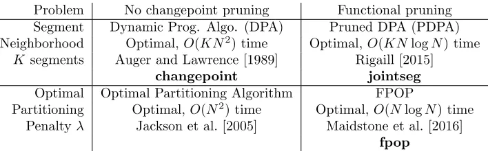
Problem No changepoint pruning Functional pruning
Segment Dynamic Prog. Algo. (DPA) Pruned DPA (PDPA)
Neighborhood Optimal,O(KN2)time Optimal,O(KNlogN)time
K segments Auger and Lawrence [1989] Rigaill [2015]
changepoint jointseg
Optimal Optimal Partitioning Algorithm FPOP
Partitioning Optimal,O(N2)time Optimal,O(NlogN)time
Penaltyλ Jackson et al. [2005] Maidstone et al. [2016]
[image:3.612.132.486.70.180.2]fpop
Table 1: Previous work on algorithms for optimal changepoint detection with no constraints between adjacent segment means.
Hocking, 2016]. These algorithms have a computational cost ofO(N) ifK increases linearly withN. The
FPOP algorithm has a computational cost that is empirically O(NlogN)in situations where K increases
sub-linearly with N. See Table 1 for a summary of the different dynamic programming algorithms and
implementations.
Whilst solving the optimal partitioning problem is faster than solving (1) for a range ofK, the drawback
is that you only get a single segmentation for a single valueKof the number of segments. Furthermore the
choice of penalty that you impose with the information criteria – which corresponds the improvement in fit to the data needed to add an additional changepoint – can be hard to tune and have an important impact on the accuracy of the estimate of the number of changepoints. One way to ameliorate this concern is to find segmentations for a range of penalties, which can be done efficiently [Haynes et al., 2017].
There are alternative approaches to fitting changepoint models, the most common of which are based on specifying a test for a single change and then repeatedly applying this test to identify multiple changepoints. Such approaches can be applied more widely than the dynamic programming based approaches described
above, and often have strong computational performance with algorithms that areO(NlogN)for the
Seg-ment Neighborhood problem. In situations where both procedures can be used, these methods are often identical if we wish to identify at most one changepoint. The advantage that the dynamic programming approaches have is that they jointly detect multiple changepoints which can lead to more accurate estimates [see e.g. Maidstone et al., 2016]. Several of these alternative algorithms are available in R. For example, the
wbspackage implements the wild binary segmentation method of Fryzlewicz [2014]. An efficient
implemen-tation of the classical binary segmenimplemen-tation heuristic is available asfpop::multiBinSeg. ThestepRpackage
implements the SMUCE algorithm for multiscale changepoint inference [Frick et al., 2014].
1.3
Models with inequality constraints between adjacent segment means
The models discussed above are unconstrained in the sense that there are no constraints between mean
parametersmk on different segments. However, as described above, constraints can be useful when data need
to be interpreted in terms of pre-defined domain-specific states. In the ChIP-seq application the changepoint model needs to be interpreted in terms of peaks (large values which represent protein binding/modification) and background (small values which represent noise).
In this context, Hocking et al. [2015] introduced a O(KN2)Constrained Dynamic Programming
Algo-rithm (CDPA) for fitting a model where up changes are followed by down changes, and vice versa (Table 2). These constraints ensure that odd-numbered segments can be interpreted as background, and even-numbered segments can be interpreted as peaks. Although the CDPA provides a sub-optimal solution to the Segment
Neighborhood problem inO(KN2)time, Hocking et al. [2016] showed that it achieves state-of-the-art peak
detection accuracy in a benchmark of ChIP-seq data sets.
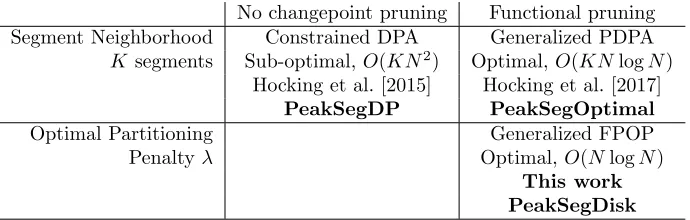
No changepoint pruning Functional pruning
Segment Neighborhood Constrained DPA Generalized PDPA
K segments Sub-optimal,O(KN2) Optimal,O(KNlogN)
Hocking et al. [2015] Hocking et al. [2017]
PeakSegDP PeakSegOptimal
Optimal Partitioning Generalized FPOP
Penaltyλ Optimal,O(NlogN)
[image:4.612.135.480.71.181.2]This work PeakSegDisk
Table 2: Algorithms for optimal changepoint detection with up-down constraints on adjacent segment means. Previous work is limited to solvers for the Segment Neighborhood problem; this paper presents Generalized Functional Pruning Optimal Partitioning (GFPOP), Algorithm 1.
Algorithm (GPDPA) reduces the number of candidate changepoints fromO(N)toO(logN)while enforcing
the constraints and maintaining optimality. The GPDPA computes the optimal solution to the up-down
con-strained Segment Neighborhood problem inO(KNlogN)time. ThePeakSegOptimalR package provides
an in-memory solver for the up-down constrained Segment Neighborhood model [Hocking et al., 2017].
1.4
Contributions
This paper presents two new algorithms for constrained optimal changepoint detection (Section 3), along with an analysis of their empirical time/space complexity in a benchmark of genomic data (Section 4). The
algorithms are implemented in the R packagePeakSegDiskon GitHub.1
First, we present a new algorithm for solving the Optimal Partitioning problem with up-down constraints between adjacent segment means (GFPOP, Algorithm 1). The fastest existing algorithm for the up-down
constrained changepoint model was the O(KNlogN) solver for the Segment Neighborhood problem
(Ta-ble 2). In large genomic data sets, we are only interested in models with many segments/changepoints, so
it is a waste of time and space to compute all models from 1 to K segments using Segment Neighborhood
algorithms. Our proposed GFPOP algorithm solves the Optimal Partitioning problem, so yields one optimal
model withKsegments (without having to compute the models from 1 toK−1segments). We show that the
empirical complexity of our GFPOP implementation is O(NlogN)time, O(NlogN) space, andO(logN)
memory, which makes it possible to compute optimal models with many peaks for typical genomic data sets on common laptop computers.
Although solving the Optimal Partitioning problem is faster by a factor of O(K), the user is unable
to directly choose the number of segments K. The user inputs a penalty λ, and gets one of the optimal
changepoint models as output. Thus, we also propose a sequential search (Algorithm 2) which computes
the optimal model for a specified number of segments K. It repeatedly calls GFPOP to solve Optimal
Partitioning with different penaltiesλ, until it finds the maximum likelihood model with at mostKsegments.
We empirically show that the sequential search only requiresO(logK)evaluations of GFPOP. Overall the
proposed algorithm is thusO(Nlog(N) log(K))time,O(NlogN)disk, O(logN)memory. In an analysis of
benchmark genomic data sets, we show that this algorithm can compute an optimal model withO(√N)>
1000peaks forN = 107data using only hours of compute time and gigabytes of storage (which is much less
than weeks/terabytes which would be required for the Segment Neighborhood solver).
2
Statistical models and optimization problems
2.1
Unconstrained Optimal Partitioning problem
Define our loss function to be the Poisson loss,`(m, z) =m−zlogm, and letλ >0 be a penalty for adding
a changepoint. Then we can infer the number of segments and the location of the changes by solving the Optimal Partitioning problem
minimize
m∈RN
N
X
i=1
`(mi, zi) +λ N−1
X
i=1
I(mi6=mi+1). (2)
The first term measures fit to the data, and the second term measures model complexity, which is proportional
to the number of changepoints. The non-negative penalty λ ∈ R+ controls the tradeoff between the two
objectives (it is a tuning parameter that must be fixed before solving the problem). Larger penaltyλvalues
result in models with fewer changepoints/segments. The extreme penalty values are λ= 0 which yieldsN
segments (N−1 changepoints), andλ=∞which yields 1 segment (0 changepoints).
Below we write an equivalent version of the Optimal Partitioning problem, in terms of changepoint
variablesci and state variablessi:
minimize
m∈RN,s∈{0}N
c∈{0,1}N−1 N
X
i=1
`(mi, zi) +λ N−1
X
i=1
I(ci = 1) (3)
subject to no change: ci= 0⇒mi=mi+1 andsi=si+1,
change: ci= 1⇒mi6=mi+1 and(si, si+1) = (0,0). (4)
Note that the state si and changepointci variables could be eliminated from the optimization problem —
si = 0and ci =I(mi 6=mi+1)for all i. We include them in problem (3) in order to show the relationship
with the problem in the next section, with constraints between adjacent segment means.
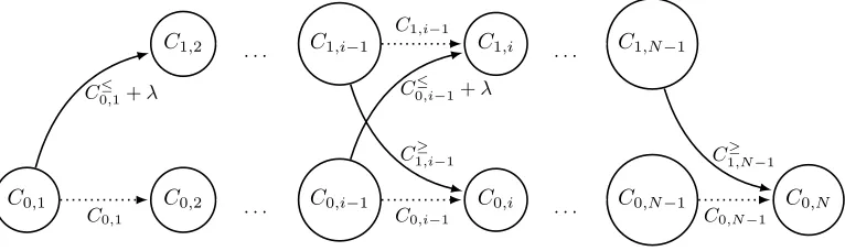
Hocking et al. [2017] proposed to use a graph to represent a constrained changepoint model. The graph that corresponds to problem (3) is shown in Figure 1, left. In such graphs, nodes represent possible values
of state variables si and edges represent possible changepoints ci 6= 0. Each edge/changepoint corresponds
to a constraint such as (4).
2.2
Optimal Partitioning problem with up-down constraints between adjacent
segment means
For genomic data such as ChIP-seq [Barski et al., 2007], it is desirable to have a changepoint model which is interpretable in terms of peaks (large values) and background noise (small values). We therefore propose
a model based on the graph shown in Figure 1, right. It has two nodes/states: s= 0for background, and
s= 1for peaks. It has two edges/changes: c= 1for a non-decreasing change from background s= 0to a
peaks= 1, and c=−1for a non-increasing change from a peak s= 1to background s= 0. Furthermore,
the model is constrained to start and end in the background state (because peaks are not present at the boundaries of genomic data sequences). Maximum likelihood inference in this model corresponds to the following minimization problem:
F(λ) = min
m∈RN,s∈{0,1}N
c∈{−1,0,1}N−1 N
X
i=1
`(mi, zi) +λ N−1
X
i=1
I(ci = 1) (5)
subject to no change: ci= 0⇒mi=mi+1 andsi=si+1,
non-decreasing change: ci = 1⇒mi≤mi+1 and(si, si+1) = (0,1),
non-increasing change: ci=−1⇒mi≥mi+1and(si, si+1) = (1,0),
s= 0
c= 1, λ s= 1
s= 0
start end
c= 1, λ,≤ c=−1,0,≥
Figure 1: State graphs for two changepoint models. Nodes represent states and solid edges represent
change-points. Left: one-state model with no constraints between adjacent segment means, problem (3). Right:
two-state model with up-down constraints between adjacent segment means, problem (5). States= 0
repre-sents background noise (small values) whereas states= 1represents peaks (large values). Constraintc= 1
enforces a non-decreasing change via the min-less operator (≤) with a penalty ofλ;c=−1enforces a
non-increasing change via the min-more operator (≥) with a penalty of0. The model is additionally constrained
to start and end in the background noises= 0 state (s1=sN = 0).
Note how the problem (5) with up-down constraints is of the same form as the previous unconstrained problem (3). Again there is one constraint for every edge/changepoint in the state graph (Figure 1). The difference is that in problem (5), we have inequality constraints between adjacent segment means (e.g. when
ci = 1, we must have a non-decreasing change in the mean mi ≤ mi+1). Another difference is the model
complexity in problem (5) is the total number of ci = 1 non-decreasing changes, which is equivalent to
the number of peak segments P, and is linear in the total number of segments K = 2P + 1 and changes
K−1 = 2P.
The solution to the Optimal Partitioning problem (5) can be computed by first solving the Segment
Neighborhood version of the problem [Maidstone et al., 2016]. In R the PeakSegDP package provides a
sub-optimal solution in O(KN2) time, and the PeakSegOptimal package provides an optimal solution
in O(KNlogN) time. However in genomic data the number of peaks/segments K increases with N, so
it is intractable to solve the Segment Neighborhood problem because both N and K are large. Therefore
in the next section we propose a new algorithm for directly solving the constrained Optimal Partitioning
problem (5), which can yield a large number of peaks inO(NlogN)time.
3
Algorithms and Software
3.1
Generalized Functional Pruning Optimal Partitioning (GFPOP)
In this section we propose a generalization of the FPOP algorithm [Maidstone et al., 2016] which allows optimal inference in models with inequality constraints between adjacent means, such as problem (5). In particular we implemented the optimal changepoint model using the Poisson loss and the up-down con-straints. The state graph (Figure 1, right) can be converted into a directed acyclic graph (Figure 2) that represents the dynamic programming updates required to solve problem (5). Each node in the computation
graph represents an optimal cost function, and each edge represents an input to themin{}operation in the
C1,i−1
C0,i−1
C1,i
C0,i C1,2
C0,2
C1,N−1
C0,N−1 C0,N C0,1
C1,i−1
C1≥,i−1
C0,i−1
C0≤,i−1+λ
C0≤,1+λ
C0,1
C1≥,N−1
C0,N−1
· · · · · ·
[image:7.612.116.499.73.187.2]· · · · · ·
Figure 2: Directed acyclic graph (DAG) representing dynamic programming computations (Algorithm 1) for changepoint model with up-down constraints between adjacent segment means. Nodes in the graph repesent cost functions, and edges represent inputs to the the MinOfTwo sub-routine (solid=changepoint, dotted=no change). There is one column for each data point and one row for each state: the optimal cost of the peak
states = 1at data point iis C1,i (top row); the optimal cost of the background noise states = 0is C0,i
(bottom row). There is only one edge going toC0,2 andC1,2 because the model is constrained to start in
the background noise state (s1= 0).
More precisely, we define the optimal cost of meanµin stateσat any data point τ∈ {1, . . . , N}to be
Cσ,τ(µ) = min
m∈Rτ,s∈{0,1}τ
c∈{−1,0,1}τ−1 τ
X
i=1
`(mi, zi) +λ τ−1
X
i=1
I(ci= 1) (6)
subject to ci= 0⇒mi=mi+1andsi =si+1,
ci= 1⇒mi≤mi+1and(si, si+1) = (0,1),
ci=−1⇒mi≥mi+1 and(si, si+1) = (1,0),
s1=sN = 0,
mτ =µ, sτ=σ. (7)
Note how the objective and constraints above are identical to the up-down constrained Optimal Partitioning
problem (5) up to τ−1 data points, but with two added constraints at data point τ (7). At data point τ
the mean is constrained to bemτ=µand the state is constrained to besτ =σ. The optimal costCσ,τ(µ)is
a real-valued function that must be computed by minimizing over all previous meansm1, . . . , mτ−1, states
s1, . . . , sτ−1, and changes c1, . . . , cτ−1. It can be computed recursively using the dynamic programming
updates that we propose below.
The algorithm begins by initializing the optimal cost of the background state at the first data point,
C0,1(µ) =`(µ, z1). (8)
The computations for the second data point are also special, because the model is constrained to start in
the background state s1 = 0. To get to the background states2 = 0 at the second data point requires no
change (c1= 0), with a cost of
C0,2(µ) =C0,1(µ) +`(µ, z2). (9)
Similarly, to get to the peak states2= 1at the second data point requires a non-decreasing change (c1= 1),
with a cost of
C1,2(µ) = min
m1≤µ
C0,1(m1) +λ+`(µ, z2) =C0≤,1(µ) +λ+`(µ, z2). (10)
Note that we were able to re-write the optimal cost function in terms of a single variable µ by using the
min-less operator,
f≤(µ) = min
The min-less operator was introduced by Hocking et al. [2017] in order to compute the optimal cost in the functional pruning algorithm that solves the Segment Neighborhood version of this problem.
More generally, the dynamic programming update rules can be derived from the computation graph
(Figure 2). The optimal cost of the peak states= 1at data i >2is
C1,i(µ) =`(µ, zi) + min{C1,i−1(µ), C0≤,i−1(µ) +λ}. (12)
Note how the inputs to the min{} operation are the same as the edges leading to the C1,i node in the
computation graph (Figure 2).
Similarly, the optimal cost of the background state s= 0is
C0,i(µ) =`(µ, zi) + min{C0,i−1(µ), C1≥,i−1(µ) +λ}, (13)
where the min-more operator is defined as
f≥(µ) = min
x≥µf(x). (14)
These dynamic programming computations are summarized in Algorithm 1, Generalized Functional Pruning Optimal Partitioning. The key to implementing the algorithm is to use a PiecewiseFunction data structure
that can exactly represent an optimal cost function Cs,i. In the case of the Poisson loss, each Cs,i(µ) is a
piecewise function where each piece is of the formαµ+βlogµ+γ. Therefore the optimal cost can be stored
as a list of intervals ofµ∈[MIN,MAX], each with coefficients α, β, γ.
Algorithm 1Generalized Functional Pruning Optimal Partitioning (GFPOP) for changepoint model with up-down constraints between adjacent segment means.
1: Input: data set z∈RN, penalty constantλ≥0.
2: Output: vectors of optimal segment meansU ∈RN and ends T∈ {1, . . . , N}N
3: Initialize2×N empty PiecewiseFunction objectsCs,i either in memory or on disk.
4: Compute minz and maxz ofz.
5: C0,1←OnePiece(z1, z, z)
6: for data pointifrom 2 toN: // dynamic programming
7: M1←λ+MinLess(i−1, C0,i−1)//cost of non-decreasing change
8: C1,i←MinOfTwo(M1, C1,i−1) +OnePiece(zi, z, z)
9: M0←MinMore(i−1, C1,i−1)//cost of non-increasing change
10: C0,i←MinOfTwo(M0, C0,i−1) +OnePiece(zi, z, z)
11: mean,prevEnd,prevMean←ArgMin(C0,n)// begin decoding
12: seg←1;Useg←mean;Tseg←prevEnd
13: while prevEnd>0:
14: if prevMean<∞: mean←prevMean
15: if seg is odd: cost←C1,prevEnd elseC0,prevEnd
16: prevEnd,prevMean←FindMean(mean,cost)
17: seg←seg+ 1;Useg←mean; Tseg←prevEnd
Discussion of pseudocode. Algorithm 1 begins on line 3 by initializing the array Cs,i of optimal cost
functions (either in memory or on disk). It then computes the min z and max z of the data (line 4) and
uses the OnePiece sub-routine to initialize the optimal cost at the first data point (line 5). Since the Poisson
loss is`(µ, z1) =µ−z1logµ, this first optimal cost function is represented as the single function piece with
interval/coefficients(α= 1, β=−z1, γ= 0,MIN=z,MAX=z).
The dynamic programming recursion in this algorithm is a loop over data points i(line 6). To compute
C1,i, the penalty constant λis added to all of the result of MinLess (line 7), before computing MinOfTwo
and does not add the penalty λ (lines 9–10). The details about how the MinLess/MinMore/MinOfTwo sub-routines process the PiecewiseFunction objects have been described previously [Hocking et al., 2017].
After computing the optimal cost functions, the decoding of optimal parameters occurs on lines 11–17.
The last segment mean and second to last segment end are first stored on line 12 in(U1, T1). For each other
segment i, the mean and previous segment end are stored on line 17 in (Ui, Ti). Note that there should
be space to store (Ui, Ti) parameters for up to N segments. In practice our implementation writes these
parameters to a text output file on disk.
Computational complexity. The complexity of Algorithm 1 is O(N I), whereI is the mean number of
intervals (function pieces) that are used to represent theCs,i cost functions. Theoretically there are some
pathological data sets for which the algorithm computesI=O(N)intervals, which results in the worst-case
complexity ofO(N2). Since the number of intervals in real data is empiricallyI=O(logN)(see Figure 5),
the overall complexity of Algorithm 1 is on averageO(NlogN). Using disk-based storage its complexity is
O(NlogN)time,O(NlogN)disk,O(logN)memory.
Usage in R. We implemented the disk-based version of Algorithm 1 in C++ code with an interface in the
R packagePeakSegDisk. To illustrate its usage we first load a set of genomic data,
> library(PeakSegDisk)
> data(Mono27ac, package="PeakSegDisk") > Mono27ac$coverage
chrom chromStart chromEnd count
1: chr11 60000 132601 0
2: chr11 132601 132643 1 3: chr11 132643 146765 0 4: chr11 146765 146807 1 5: chr11 146807 175254 0
---6917: chr11 579752 579792 1 6918: chr11 579792 579794 2 6919: chr11 579794 579834 1 6920: chr11 579834 579980 0 6921: chr11 579980 580000 1
>
Note that the 4 column bedGraph format shown above must be used to represent a data set. Futhermore a run-length encoding should be used for data sets that have runs of the same values. Each row represents a sequence of identical data values. For example the first row means that the value 0 occurs on the 72601 positions in [60000,132601), the second row means a value of 1 for the 42 positions in [132601,132643), etc. This run-length encoding results in significant savings in disk space and time [Cleynen et al., 2014]; for example in the data set above there are only 6921 lines used to represent 520000 data values.
In order to handle very large data sets while using only O(logN) memory, the algorithm reads input
data from a text file on disk (and never actually stores the entire data set in memory). So before using the algorithm we must save the data set to disk, in bedGraph format (the four columns shown above, separated
by tabs). Note that the file name must becoverage.bedGraph:
> data.dir <- file.path("Mono27ac", "chr11:60000-580000") > dir.create(data.dir, showWarnings=FALSE, recursive=TRUE) > write.table(
After saving the file to disk, we can run the algorithm using the code below:
> ## Compute one model with penalty=10000
> fit <- PeakSegDisk::problem.PeakSegFPOP(data.dir, "10000") >
For the first argument you must give the folder name (not the coverage.bedGraph file name) to the
problem.PeakSegFPOP function. Note that the second argument must be a character string that represents
a penalty value (non-negative real number, larger penalties yield fewer peaks). The smallest value is "0"
which yields max peaks, and the largest value is"Inf" which yields no peaks. It must be an R character
string (not a real number) because that string is used to create files which are used to store/cache the results. If the files already exist (and are consistent) then problem.PeakSegFPOP just reads them; otherwise it runs the dynamic programming C++ code in order to create those files.
The returned fit object is a named list of data.tables. The fit$losscomponent shown below is one
row that contains general information about the computed model:
> fit$loss
penalty segments peaks bases mean.pen.cost total.loss equality.constraints
1: 10000 15 7 520000 0.2189332 43845.26 0
mean.intervals max.intervals
1: 14.42581 41
>
Above we can see that the optimal model for λ= 104 hadP = 7peaks (K= 15 segments/K−1 = 14
changepoints). The fit$segments component is used to visualize three of those peaks in a subset of the
data below.
> library(ggplot2)
> gg <- ggplot()+theme_bw()+
+ geom_step(aes(chromStart, count), color="grey50", data=Mono27ac$coverage)+ + geom_segment(aes(chromStart, mean, xend=chromEnd, yend=mean),
+ color="green", size=1, data=fit$segments)+ + coord_cartesian(xlim=c(2e5, 3e5))
> print(gg) >
0 10 20 30 40
200000 225000 250000 275000 300000
chromStart
3.2
Sequential search algorithm for
P
∗peaks
Note that in GFPOP (Algorithm 1), the user inputs a penaltyλ, and is unable to directly choose the number
of segments/peaks. In this section, we propose an algorithm that allows the user to specify the number of peaks. The algorithm then repeatedly calls GFPOP until it finds the most likely model with at most the specified number of peaks.
To understand how the algorithm works, we must review the relationship between the Optimal Parti-tioning and Segment Neighborhood problems [Maidstone et al., 2016]. We define the optimal loss for a given
number of peaksP as
LP = min
m∈RN,s∈{0,1}N
c∈{−1,0,1}N−1 N
X
i=1
`(mi, zi) (15)
subject to ci= 0⇒mi=mi+1 andsi=si+1,
ci= 1⇒mi≤mi+1 and(si, si+1) = (0,1),
ci=−1⇒mi ≥mi+1and (si, si+1) = (1,0),
s1=sN = 0,
P= N−1
X
i=1
I(ci= 1). (16)
The problem above is the Segment Neighborhood version of the Optimal Partitioning problem that GFPOP
solves (5). The penalty λ is absent, and the model complexity (the number of peaks) has moved to a
constraint (16). Recall thatF(λ)is the minimum value of the Optimal Partitioning problem (5). It can be
written in terms of the solution to the Segment Neighborhood problem (15),
F(λ) = min P∈{0,1,...,Pmax}
LP+λP. (17)
The equation above makes it clear that there are only a finite number of optimal changepoint models (from
0 to Pmax peaks). F(λ) is a concave, non-decreasing function that can be computed as the minimum of a
finite number of affine functionsfP(λ) =LP +λP.
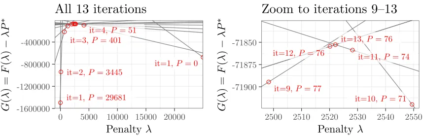
We now assume the user wants to compute the optimal model with a fixed number of peaks P∗. To
compute that model we will maximize the function
G(λ) =F(λ)−P∗λ= min P∈{0,1,...,Pmax}
LP+λ(P−P∗)
| {z }
gP(λ)
. (18)
From the equation above it is clear thatG(λ)is a concave function that can be computed as the minimum
of a finite number of affine functionsgP(λ) =LP+λ(P−P∗). For an exampleGfunction see Figure 3.
Discussion of pseudocode. Algorithm 2 summarizes the sequential search. The main idea of the
sequen-tial search algorithm is to keep track of a lower boundp < P∗ and upper boundp > P∗ on the number of
peaks computed thus far. The algorithm starts withλ= 0,p=Pmax (line 2) andλ=∞, p= 0(line 3). At
each iteration of the algorithm, we find the intersection of the affine functionsgp(λ) =gp(λ), which leads to
a new candidate penalty λnew = (Lp−Lp)/(p−p)(line 5). As previously described [Haynes et al., 2017],
there are two possibilities for the solution to the Optimal Partitioning problem:
• GFPOP(λnew) yieldsporppeaks (line 7). In that casemaxλG(λ) =G(λnew) =gp(λnew) =gp(λnew)
and there is no Optimal Partitioning model with P∗ peaks. We terminate the algorithm by returning
the model withppeaks.
• GFPOP(λnew) yields a new model with pnew peaks. If pnew = P∗ then maxλG(λ) = LP∗ and we
return this model (line 8). Otherwise it must be true thatp < pnew< p. Ifp < pnew< P∗ then we use
it=1,P = 29681
it=1,P = 0
it=2,P= 3445
it=3,P= 401
it=4,P= 51
-1600000 -1200000 -800000 -400000
0 5000 10000 15000 20000
Penalty
λ
G
(
λ
)
=
F
(
λ
)
−
λP
∗
All 13 iterations
it=9,P= 77
it=10,P = 71
it=11,P= 74
it=12,P = 76
it=13,P= 76
-71900 -71875 -71850
2500 2510 2520 2530 2540 2550
Penalty
λ
G
(
λ
)
=
F
(
λ
)
−
λP
∗
[image:12.612.93.522.74.212.2]Zoom to iterations 9–13
Figure 3: Example of aG(λ) function which is maximized in order to find the most likely model with at
mostP∗= 75peaks. Red dots showG(λ)values evaluated by the algorithm; grey lines show affine functions
gP(λ) =LP+ (P−P∗)λused to determine the nextλvalue (line 5 of Algorithm 2). Left: iteration 1 runs
GFPOP with λ ∈ {0,∞}, resulting in initial lower bound of p= 0 peaks and upper bound of p= 29681
peaks. In iteration 2 the algorithm finds the intersection of the upper/lower bound linesg0(λ) =g29681(λ)
at λ= 90.9; running GFPOP with that penalty reduces the upper bound to p= 3445. Right: In the last
iteration (13), we run GFPOP with λ= 2522.1 (which is where g74 intersects g76), resulting in 76 peaks
when we already have p= 76 as an upper bound (computed in iteration 12). The maximum of Gis thus
G(2522.1) =g74(2522.1) =g76(2522.1); the algorithm returns the model withP = 74peaks.
Algorithm 2Sequential search forP∗peaks using GFPOP.
1: Input: dataz∈RN, target peaksP∗.
2: L, p←GFPOP(z, λ= 0)// initialize upper bound to max peak model
3: L, p←GFPOP(z, λ=∞)// initialize lower bound to 0 peak model
4: WhileP∗6∈ {p, p}:
5: λnew= (L−L)/(p−p)
6: Lnew, pnew←GFPOP(z, λnew)
7: Ifpnew∈ {p, p}: return model withppeaks.
8: Ifpnew=P∗: return model withpnew peaks.
9: Ifpnew< P∗: L, p←Lnew, pnew // new lower bound
10: Else: L, p←Lnew, pnew // new upper bound
Computational complexity. The space complexity is the same as GFPOP:O(NlogN)disk andO(logN)
memory. Its time complexity is linear in the number of iterations of the while loop (line 4). Empirically we
seeO(logP∗)iterations (Section 4.4), which implies an overall time complexity ofO(Nlog(N) log(P∗)).
Usage in R. The R code below computes the optimal model with 17 peaks:
> ## Compute the optimal model with 17 peaks.
> fit <- PeakSegDisk::problem.sequentialSearch(data.dir, 17L) >
If you want to see how many iterations/penalties the algorithm required in order to compute the optimal
model with 17 peaks, you can look at thefit$otherscomponent:
> fit$others[, list(iteration, under, over, penalty, peaks, total.loss)]
iteration under over penalty peaks total.loss
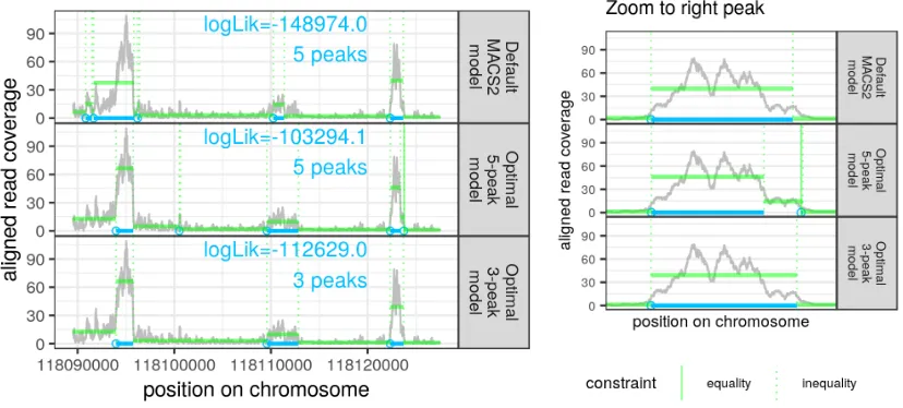
Figure 4: One ChIP-seq data set with three peak models. (green horizontal segment means; green dotted
vertical lines for changepoints; blue bars for peaks; blue dots for peak starts)Top: the MACS2 algorithm (a
heuristic from the bioinformatics literature) computed a sub-optimal model with five peaks for these data. Middle: the most likely model with five peaks contains one equality constraint between segment means (see
zoomed figure on the right), which suggests that there are less than five easily interpretable peaks. Bottom:
the most likely model with three peaks is also more likely than the MACS2 model.
2: 1 NA NA Inf 0 375197.873
3: 2 0 3199 157.9947 224 -62199.931
4: 3 0 224 1952.6688 17 2640.128
>
The output above shows that the algorithm only used three iterations to compute the optimal model
with 17 peaks. Theunder and overcolumns show the current values of pand p, respectively. The peaks
andtotal.lossarepnew, Lnewfrom the model that resulted from running GFPOP withλ=penalty. Note
that iteration 1 evaluates both extreme penaltiesλ∈ {0,∞}in parallel (andλ=∞is the trivial model with
0 peaks that can be computed without dynamic programming), so these two models are considered a single iteration.
4
Results on genomic data
In this section we discuss several applications of our algorithms in some typical genomic data sets. We
downloaded thechipseqdata set from the UCI machine learning repository [Newman and Merz, 1998]. We
considered 4951 data sets ranging in size from N = 103 to N = 107 data points to segment (lines in the
bedGraph file).
4.1
Application: Computing the maximum likelihood model with a given
num-ber of peaks
● 4,583,432 data, 512 intervals
● 11,499,958 data, 19 intervals
mean
max
10 100 1000
10000 1e+05 1e+06 1e+07
N = data to segment (log scale)
Inter
v
als/candidate changepoints
(log scale)
1 gigabyte
●
8,521,917 data, 86 gigabytes
1 hour
●
10,289,916 data, 190 minutes
gigab
ytes
min
utes
10000 1e+05 1e+06 1e+07 0.1
10 1000
0.1 10 1000
N = data to segment (log scale)
Computational requirements
[image:14.612.92.480.68.220.2](log scales)
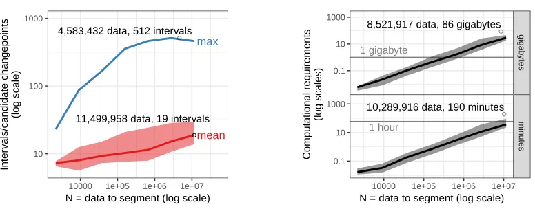
Figure 5: In our empirical tests, the computational requirements of the GFPOP algorithm were log-linear
O(NlogN) in the number of data points N to segment. Left: we analyzed the number of intervals I
(candidate changepoints) stored in the Ct(µ) cost functions, because the total time/space complexity is
O(N I). We observed empirically that the mean number of intervals I = O(logN) (red curve). Even
the maximum number of intervals (blue curve) is much less than N. Right: storage on disk (top panel)
and computation time (bottom panel) are empirically O(NlogN). Error bands show median and 5%/95%
quantiles over several data sets of a given sizeN; black dots and text show computational requirements for
the most extreme data sets.
bioinformatics literature [Zhang et al., 2008]. It detects five peaks, so we ran Algorithm 2 withP∗ = 5on
these data in order to compute the most likely model with at most 5 peaks (shown in middle panel). It is clear that the optimal 5 peak model is a better fit in terms of likelihood (as expected); it is also a better fit visually, especially for the peak on the left. Furthermore the optimal 5 peak model actually has one equality constraint between adjacent segment means, suggesting that there are less than five easily interpretable peaks. Therefore we also computed the optimal 3 peak model (bottom panel), which also has a higher log-likelihood than the 5 peak MACS2 model. Overall it is clear that our algorithms can be used to compute models which are both more likely and simpler (with fewer peaks) than heuristics such as MACS2.
4.2
GFPOP is empirically log-linear
To measure the empirical time complexity of GFPOP (Algorithm 1), we ran it on all 4951 genomic data sets,
with a grid of penalty valuesλ∈(logN, N)for each data set of sizeN. The overall theoretical time/space
complexity isO(N I), whereIis the number of intervals (candidate changepoints) stored in theCs,toptimal
cost functions. During each run we therefore recorded the mean and max number of intervals over all s, t.
We observed that the empirical mean/max number of intervals increases logarithmically with data set size,
I =O(logN) (Figure 5, left). Remarkably, for the largest data set (N = 11,499,958) the algorithm only
computed a mean of I = 19 intervals. The most intervals computed to represent any single Cs,t function
was 512 intervals for one data set withN = 4,583,432.
Since empiricallyI=O(logN)in these genomic data sets, we expected an overall time/space complexity
ofO(NlogN). The empirical measurements of time and space requirements are consistent with this
expec-tation (Figure 5, right). For the largest data sets (N = 107), the algorithm takes only about 80 gigabytes of
storage and 1 hour of computation time. Overall these results suggest that GFPOP can be used to compute
optimal peak models for genomic data inO(NlogN)space/time.
4.3
Disk storage is slower than memory by a constant factor
In the previous section, we discussed how tens of gigabytes of storage are required to run GFPOP when
memory disk
1 10 100
1e+04 1e+05 1e+06
N = number of data to segment (log scale)
seconds (log scale)
● ● ● ● ● ● ● ● ● ● ● ● ● ● ● ● ● ● ● ● ● ● ● ● ● ● ● ● ● ● ● ● ● ● ● ● ● ● ● ● ● ● ● ● ● ● ● ● ● ● ● ● ● ● ● ● ● ● ● ●● ● ● ● ● ● ● ● ● ● ● ● ● ● ● ● ● ● ● ● ● ● ● ● ● ● ● ● ● ● ● ● memory disk 10 20 30
1e+02 1e+03 1e+04 1e+05
lambda=penalty (log scale)
seconds (log scale)
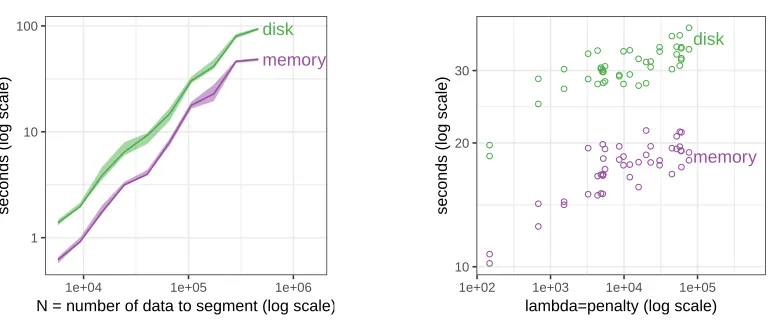
Figure 6: The disk-based storage method is only a constant factor slower than the memory-based method.
We benchmarked both methods on several small data sets (N ≤462,890) for which optimal models could
be computed using 1GB of storage. Left: computation time is empirically O(NlogN) for both storage
methods, but the disk-based method is slower by a constant factor. Median line and quartile band computed
over several penalty values for a given data set. Right: fixing one data set data set withN = 106,569, the
computation time increases with penalty valueλfor both storage methods.
storage. We compared our disk-based implementation to another memory-based implementation, in terms
of computation time on small data sets for which GFPOP uses <1GB of storage. We observed that disk
storage is slower than memory storage by a constant factor (1.7–2.3×, Figure 6), which was expected.
4.4
Sequential search is faster than Segment Neighborhood
In this section we compare the number of O(NlogN) dynamic programming iterations required for the
proposed sequential search (Algorithm 2) and the previous Generalized Pruned Dynamic Programming Al-gorithm (GPDPA) of Hocking et al. [2017]. Both alAl-gorithms compute the solution to the Segment
Neighbor-hood problem (optimal model with at mostPpeaks). The GPDPA requires exactly2P iterations of dynamic
programming, each of which is anO(NlogN) operation. In contrast, the proposed sequential search
(Al-gorithm 2) needs to solve for a sequence of penalties, each of which is done via GFPOP in O(NlogN)
time.
For two data sets withN ≈106we therefore recorded the empirical number of times GFPOP was called
by the sequential search algorithm. We observed that the number of GFPOP calls grows logarithmically
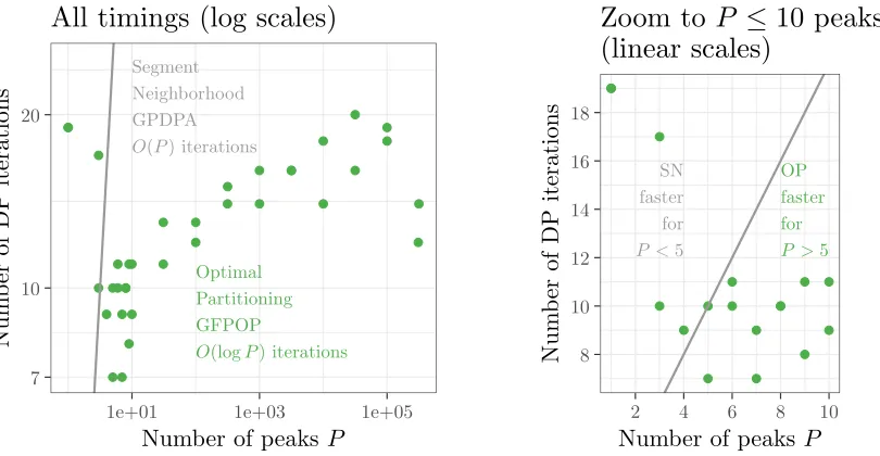
withP (Figure 7, left). For a large number of peaks (P >5), it is clearly faster to use the sequential search
algorithm (Figure 7, right). Overall these experiments indicate that the time complexity of the sequential
search in genomic data isO(Nlog(N) log(P))forN data and P peaks.
4.5
Application: computing a zero-error peak model
In this section we study the perfomance of the proposed algorithms in a typical application. In the UCI
chipseqdata set, there are labels that indicate subsets of the data with or without peaks. In this context the labels can be used to compute false positive and false negative rates for any peak model. For example Figure 8 shows one data set with six labels and four peak models computed via GFPOP. Small penalties result in too many peaks, and large false positive rates. Large penalties result in too few peaks, and large false negative rates. A range of intermediate penalties/peaks achieves zero label errors. The labels can thus be used to determine an appropriate number of peaks (with zero errors) for each data set.
[image:15.612.94.481.68.228.2]Segment Neighborhood GPDPA
O(P)iterations
Optimal Partitioning GFPOP
O(logP)iterations
7 10 20
1e+01 1e+03 1e+05
Number of peaks
P
Nu
m
b
er
of
D
P
ite
rati
on
s
All timings (log scales)
SN faster for
P <5
OP
faster for
P >5
8 10 12 14 16 18
2 4 6 8 10
Number of peaks
P
Nu
m
b
er
of
D
P
ite
rat
ion
s
[image:16.612.98.503.75.285.2]Zoom to
P
≤
10
peaks
(linear scales)
Figure 7: Comparison of time to compute optimal model with at most P peaks using Segment
Neigh-borhood (grey lines) and Optimal Partitioning with proposed sequential search (green dots). GFPOP with
sequential search (Algorithm 2) was used to compute optimal models with different numbers of peaks P,
for two data sets with N ≈106. Left: the number of iterations is linearO(P)for Segment Neighborhood
(grey line) but empirically O(logP) for Optimal Partitioning with sequential search (green dots). Right:
Optimal Partitioning is empirically faster for computing models withP >5 peaks (10 segments); Segment
Neighborhood is faster for smaller models.
● ● ● ● ● ● ● ● ● ● ● ● ● ● ● ● ● ● ● ● ● ● ● ● ● ● ● ● penalty=6682 penalty=9586 penalty=267277 penalty=278653
too many peaks (320) no errors, max peaks (236) no errors, min peaks (34) too few peaks (33)
0 10 20 30
15500000 16000000 16500000 17000000
position on chromosome
aligned read counts
error type correct false negative false positive label peakEnd peakStart
Figure 8: Labels are used to compute an error rate for each peak model (blue bars), defined as the sum of
false positive and false negative labels (rectangles with black outline). This H3K36me3 ChIP-seq data set
hasN = 1,254,751data to segment on a subset of chr12, but in the plot above we show only the 82,233 data
(grey signal) in the region around the labels (colored rectangles). The model with penalty=6682 results in 320 peaks, which is too many (three false positive labels with more than one peak start/end). Conversely, the model with penalty=278653 results in 33 peaks, which is too few (only two peaks in the plotted region, resulting in two false negative labels on the right where there should be exactly one peak start/end). The range of penalties between 9586 and 267277 results in models with between 34 and 236 peaks, and achieves zero label errors.
errors (34/236 in Figure 8), along with the mean of those two values,(34 + 236)/2 = 135. We plot the mean
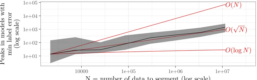
[image:16.612.123.488.391.524.2]O(N
)
O(log
N
)
O(
√
N
)
1e+01 1e+02 1e+03 1e+04 1e+05
10000 1e+05 1e+06 1e+07
N = number of data to segment (log scale)
P
eak
s
in
mo
d
el
s
wi
th
mi
n
lab
el
err
or
(l
og
sc
ale
[image:17.612.95.517.75.207.2])
Figure 9: The model with minimal label errors has O(√N) peaks in a data set of sizeN. For each data
set we computed peak models with minimal label errors (see Figure 8); we then plot the number of peaks in
minimal error models as a function of data set sizeN. Black median line and grey quartile band computed
over several data sets of a given sizeN; asymptotic reference lines shown in red.
clear that models withO(√N)peaks achieve zero label errors.
Computing the optimal model withO(√N)peaks is computationally expensive using the Segment
Neigh-borhood algorithm (PeakSegOptimalpackage), because the overall complexity would be O(N√NlogN).
For example inN = 107 data,P=O(√N) = 1414peaks achieves zero label errors. Computing the optimal
model with Segment Neighborhood would thus require 2828 O(NlogN) DP iterations. If we assume that
each iteration would have similar computational requirements as oneO(NlogN)run of GFPOP, each would
require about 1 hour and 80 gigabytes (Figure 5). Overall that would mean 220 terabytes of storage and 17 weeks of computation time, which is much too expensive in practice.
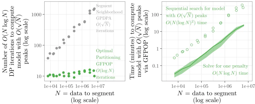
Instead, we can use the proposed sequential search (Algorithm 2) to compute a zero-error model with
O(√N)peaks. In our empirical tests, we observed that onlyO(logN)GFPOP calls are required to compute
O(√N)peaks (Figure 10, left). In particular forN= 107data only 10–15 GFPOP calls are required, which
is significantly fewer than the 2828 DP iterations that would be required for the Segment Neighborhood
solver in thePeakSegOptimalpackage.
We also observed that the empirical timings of the sequential search are only a log-factor slower than
solving for one penalty (Figure 10, right). In particular forN = 107data the sequential search takes on the
order of hours, which is much less than the weeks that would be required to solve the Segment Neighborhood
problem. Overall these empirical results indicate that the sequential search algorithm in thePeakSegDisk
package can be used to compute a model withO(√N)peaks inO(N(logN)2)time.
5
Summary and discussion
This paper presented two new algorithms for constrained optimal changepoint detection. We presented Generalized Functional Partitioning Optimal Partitioning (GFPOP) which computes the optimal model for
one penalty λ. We also proposed a sequential search algorithm which repeated calls GFPOP in order to
compute the most likely model with at mostP peaks.
We analyzed the proposed algorithms by running them on a set of genomic data sets ranging fromN = 103
to N = 107. First, we showed that the algorithms can be used to compute models which are more likely
than existing heuristics, and often simpler (fewer peaks).
Second, we studied the empirical complexity of GFPOP as the a function of the number of data N. We
showed that GFPOP requiresO(NlogN)time, O(NlogN)space, andO(logN)memory. We furthermore
showed that using disk-based storage is only a constant factor slower than memory-based storage. Overall
Optimal Partitioning GFPOP O(logN)
iterations
Segment Neighborhood GPDPA O(√N)
iterations
10 100 1000
1e+04 1e+05 1e+06 1e+07
N
= data to segment
(log scale)
Nu
m
b
er
of
O
(
N
log
N
)
D
P
it
erat
ion
s
to
com
pu
te
mo
d
el
wi
th
O
(
√
N
)
p
eak
s
(l
og
sc
al
e)
Sequential search for model
withO(√N)peaks
O(N(logN)2)time
Solve for one penalty
O(NlogN)time 0.1
1 10 100
1e+04 1e+05 1e+06 1e+07
[image:18.612.90.530.75.255.2]N
= data to segment
(log scale)
Ti
me
(mi
n
u
tes
)
to
comp
ut
e
mo
d
el
wi
th
O
(
√
N
)
p
eak
s
v
ia
GF
P
O
P
(l
og
sc
ale
)
Figure 10: Computing a zero-error model with O(√N) peaks is possible in O(N(logN)2) time using
our proposed Optimal Partitioning Search algorithm. Left: Segment Neighborhood requires O(√N)
dy-namic programming iterations to compute a model withO(√N)peaks; our proposed Optimal Partitioning
search algorithm requires only O(logN)iterations. Right: Optimal Partitioning solves for one penalty in
O(NlogN) space/time (median line and 5%/95% quantile band over data sets and penalties); finding the
zero-error model withO(√N)peaks takesO(N(logN)2)time/space – only a log factor more (points).
amounts of time (minutes).
Third, we studied the empirical complexity of sequential search as a function of data size N and number
of peaks P. We showed that it requires O(Nlog(N) log(P)) time, O(NlogN)disk, O(logN) memory. In
particular we showed that it is always faster than Segment Neighborhood solvers for models with P > 5
peaks.
Finally we analyzed the labels in our benchmark of genomic data, which indicated that an appropriate
number of peaks isP =O(√N). We showed that sequential search computes the model withO(√N)peaks
in O(N(logN)2) time, whereas existing Segment Neighborhood algorithms would be O(N√NlogN). We
showed that forN= 107data our approach only requires hours/gigabytes of time/space to compute optimal
models. Our algorithms thus make it practical for the first time to compute optimal models with many peaks for genomic data sets.
Reproducible research statement. The source code and data used to create this manuscript (including
all figures) is available athttps://github.com/tdhock/PeakSegFPOP-paper
References
I. Auger and C. Lawrence. Algorithms for the optimal identification of segment neighborhoods. Bull Math
Biol, 51:39–54, 1989.
A. Barski, S. Cuddapah, K. Cui, T.-Y. Roh, D. E. Schones, Z. Wang, G. Wei, I. Chepelev, and K. Zhao.
High-resolution profiling of histone methylations in the human genome. Cell, 129(4):823–837, 2007.
J. D. Buenrostro, B. Wu, H. Y. Chang, and W. J. Greenleaf. ATAC-seq: A Method for Assaying Chromatin
Accessibility Genome-Wide. Current Protocols in Molecular Biology, 2015.
H. Choi, A. I. Nesvizhskii, D. Ghosh, and Z. S. Qin. Hierarchical hidden markov model with application to
A. Cleynen, M. Koskas, E. Lebarbier, G. Rigaill, and S. Robin. Segmentor3IsBack: an R package for the
fast and exact segmentation of Seq-data. Algorithms for Molecular Biology, 9:6, 2014.
K. Frick, A. Munk, and H. Sieling. Multiscale change point inference.Journal of the Royal Statistical Society:
Series B (Statistical Methodology), 76(3):495–580, 2014.
P. Fryzlewicz. Wild binary segmentation for multiple change-point detection. 42, 11 2014.
K. Haynes, I. A. Eckley, and P. Fearnhead. Computationally efficient changepoint detection for a range of
penalties. Journal of Computational and Graphical Statistics, 26(1):134–143, 2 2017. ISSN 1061-8600.
T. Hocking, G. Rigaill, P. Fearnhead, and G. Bourque. A log-linear time algorithm for constrained change-point detection. arXiv:1703.03352, 2017.
T. D. Hocking, G. Rigaill, and G. Bourque. PeakSeg: constrained optimal segmentation and supervised
penalty learning for peak detection in count data. InProc. 32nd ICML, pages 324–332, 2015.
T. D. Hocking, P. Goerner-Potvin, A. Morin, X. Shao, T. Pastinen, and G. Bourque. Optimizing chip-seq
peak detectors using visual labels and supervised machine learning. Bioinformatics, 2016.
B. Jackson, J. Scargle, D. Barnes, S. Arabhi, A. Alt, P. Gioumousis, E. Gwin, P. Sangtrakulcharoen, L. Tan,
and T. Tsai. An algorithm for optimal partitioning of data on an interval. IEEE Signal Process Lett, 12:
105–108, 2005.
N. A. Johnson. A Dynamic Programming Algorithm for the Fused Lasso and L0-Segmentation. Journal of
Computational and Graphical Statistics, 22(2):246–260, 2013.
R. Killick, P. Fearnhead, and I. A. Eckley. Optimal detection of changepoints with a linear computational
cost. Journal of the American Statistical Association, 107(500):1590–1598, 2012.
R. Maidstone, T. Hocking, G. Rigaill, and P. Fearnhead. On optimal multiple changepoint algorithms for
large data. Statistics and Computing, pages 1–15, 2016. ISSN 1573-1375.
A. Cleynen and E. Lebarbier. Segmentation of the Poisson and negative binomial rate models: a penalized
estimator. ESAIM: PS, 18:750–769, 2014.
C. B. D. Newman and C. Merz. UCI repository of machine learning databases, 1998.
M. Pierre-Jean, G. Rigaill, and P. Neuvial. Performance evaluation of DNA copy number segmentation
methods. Briefings in Bioinformatics, 2015.
G. Rigaill. A pruned dynamic programming algorithm to recover the best segmentations with 1 to kmax
change-points. Journal de la Soci´et´e Fran¸caise de la Statistique, 156(4), 2015.
G. Rigaill and T. D. Hocking. fpop: Segmentation using Optimal Partitioning and Function Pruning, 2016.
URLhttps://R-Forge.R-project.org/projects/opfp/. R package version 2016.10.25/r55.
Y. Zhang, T. Liu, C. A. Meyer, J. Eeckhoute, D. S. Johnson, B. E. Bernstein, C. Nusbaum, R. M. Myers,