Numerical Treatment of Initial Boundary Value Problems with Mixed Boundary Conditions

(1)

ISSN Online: 2161-1211 ISSN Print: 2161-1203

DOI: 10.4236/ajcm.2018.82012 Jun. 28, 2018 153 American Journal of Computational Mathematics

Numerical Treatment of Initial-Boundary Value

Problems with Mixed Boundary Conditions

Nawal Abdullah Alzaid, Huda Omar Bakodah

Department of Mathematics, King Abdulaziz University, Jeddah, KSA

Abstract

In this paper, we extend the reliable modification of the Adomian Decompo-sition Method coupled to the Lesnic’s approach to solve boundary value problems and initial boundary value problems with mixed boundary condi-tions for linear and nonlinear partial differential equacondi-tions. The method is ap-plied to different forms of heat and wave equations as illustrative examples to exhibit the effectiveness of the method. The method provides the solution in a rapidly convergent series with components that can be computed iteratively. The numerical results for the illustrative examples obtained show remarkable agreement with the exact solutions. We also provide some graphical repre-sentations for clear-cut comparisons between the solutions using Maple soft-ware.

Keywords

Decomposition Method, Modified Adomian Decomposition Method, Linear and Nonlinear Partial Differential Equations, Mixed Boundary Conditions, Initial-Boundary Value Problem

1. Introduction

Mixed boundary value problems are characterized by a combination of Dirichlet and Neumann conditions along at least one boundary condition. They occur in a wide range of engineering and applied mathematics applications [1][2][3][4]. These applications include the classic electrical potential and electric field condi-tions on a disk [5], stress and strain conditions around a punch pressing on an elastic surface [6] as well as some applications in porous media problems such as the infiltration and seepage among others [7][8]. Historically, only very few of these problems could be solved using analytic methods. In view of this, many researchers obtained the solutions of initial and boundary value problems by How to cite this paper: Alzaid, N.A. and

Bakodah, H.O. (2018) Numerical Treat-ment of Initial-Boundary Value Problems with Mixed Boundary Conditions. Ameri-can Journal of Computational Mathemat-ics, 8, 153-174.

https://doi.org/10.4236/ajcm.2018.82012

Received: April 11, 2018 Accepted: June 25, 2018 Published: June 28, 2018

http://creativecommons.org/licenses/by/4.0/

(2)

DOI: 10.4236/ajcm.2018.82012 154 American Journal of Computational Mathematics

using either initial or boundary condition(s). In recent years, there have been significant developments in the use of various semi-analytical methods for par-tial differenpar-tial equations such as the homotopy perturbation method [9] and Adomian Decomposition Method (ADM) [10]. Duan and Rach [11] developed a new resolution method of Boundary Value Problems (BVPs) for nonlinear or-dinary differential equations using the ADM. It is also well-known that the ADM provides approximate analytic solutions without using the Green function con-cept, which greatly facilitates analytic approximations and numerical computa-tions. Several different resolution techniques for solving BVPs for nonlinear or-dinary differential equations by using the ADM were considered by Adomian and Rach [12]-[18], Adomian [19], and Wazwaz [20]-[26]. Also, for a two-point BVP for second-order nonlinear differential equations, Adomian and Rach [17] [18] proposed the double decomposition method in order to avoid solving such nonlinear algebraic equations, and Jang [27] and Ebaid [28] introduced different modified inverse linear operators. Adomian [29] suggested a modified method for the hyperbolic, parabolic and elliptic partial differential equations with initial and boundary conditions by using two equations for u, one inverting the Lt operator and the other inverting the Lx operator, then, adding them and di-viding by two. Further, with regards to the mixed value problems, Lesnic and Elliot

[30] proposed the inverse operator defined by

0

1

1 d d

x x

L− ₌ x_′ x_′′

∫ ∫

to solve the

linear homogeneous heat equationu u xt = xx, 0< <x 1,t>0 subject to the mixed boundary conditions u x t

( )

, =h t1

( )

, ux

( )

1,t =h t2

( )

, where

β

i=

( ), 1,2

t i= are known functions. However, in this paper, we will present a modified recur-sion scheme based on the reliable modification of the ADM with new structure of the inverse operator applied to the (BVPs) with mixed boundary conditions using Lesnic’s approach and Ebaid’s method. The proposed operator allows the appearance of all the conditions in the solution thereby making the solution more realistic. The paper is arranged in the following manner: in Section 2, we analyze the ADM; Section 3 presents the modified ADM suggested by Wazwaz; in Section 4, Lesnic’s approach is used to approximate solutions of some prob-lems; the implementation of this new method to some test problems is presented in Section 5; finally, a brief conclusion is given in Section 6.

2. Analysis of the Adomian Decomposition Method with

Mixed Conditions

Nonlinear partial differential equations models in mathematics and physics play an important role in theoretical sciences. The understanding of these nonlinear partial differential equations is also crucial to many applied areas such as mete-orology, oceanography, and aerospace industry. Nonlinear partial differential equations are the most fundamental models in studying nonlinear phenomena.

Consider the nonlinear partial differential equation given in an operator form

( )

,

( )

,

( )

,

( )

,

( )

,

x t

(3)

where Lx and Lt are the linear operators to be inverted, which are usually the highest order differential operators in x, and t respectively; Lx, R is the linear remainder operator; Nu x t

( )

, is a nonlinear operator which is assumed to be analytic function, and g x t

( )

, is the input function that is assumed to be con-tinuous function. The solutions for u x t

( )

, obtained from the operator equa-tions L ux in x-direction and L ut in t-direction are called partial solutions. We further give the following illustrations:

2.1. Boundary Value Problems

Consider the general form of the single second-order nonlinear inhomogeneous temporal-spatial partial differential equation:

( )

,

( )

,

( )

,

( )

, , , 0,

xx tt

L u x t +L u x t +Nu x t =g x t a x b t≤ ≤ > _(2.2) subject to the mixed boundary conditions

( )

, 1

( ) ( )

, x , 2

( )

u a t =h t u b t =h t (2.3)

where, L u x txx

( )

, _x22u x t L u x t

( )

, , tt

( )

, _t22u x t

( )

,

∂ ∂

= =

∂ ∂ . We consider the x partial

solution as

( )

,

( )

,

( )

,

( )

,

xx tt

L u x t =g x t −L u x t −Nu x t (2.4)

Applying the two-fold indefinite integration inverse operator 1 _{d d}

xx

L− ₌

_{∫ ∫}

x x_′

to both sides of Equation (2.4), gives

( )

_, 1

( )

_, 1

( )

_, 1

( )

_{, ,}

x xx xx tt xx

u x t _{= Φ +}L g x t− ₋L L u x t− ₋L Nu x t− _(2.5)

where Φ =x c t c t x1

( )

+ 2

( )

and the constants of integrations c t1

( )

and c t2

( )

, are determined from the boundary conditions. We now decompose the follow-ing Φx, the linear and nonlinear terms u and Nu based on ADM as follows:

( )

(

)

, 1, 2,

0 0 ,

x x n n n

n n c t c t x

∞ ∞

= =

Φ =

∑

Φ =

∑

+

( )

0

, n , ,

n

u x t ∞ u x t

=

∑

( )

(

0 1 2

)

0

, n , , , , n

n

Nu x t ∞ A u u u u

=

∑

 (2.6)

where An’s are the Adomian polynomials determined from the definitional formula

0 ₀

1 d _, _0.

! d

n

k

n n k

k

A N u n

n λ λ _λ

∞

= ₌

 

= _ _ ≥



∑

 (2.7)

Substituting Equation (2.6) into Equation (2.5), yields the following recursion scheme

( )

1

0 x,0 xx , ,

u _{= Φ +}L g x t−

1 1

1 , 1 , 0.

n x n xx tt n xx n

u L L u− L A n−

+ = Φ + − − ≥ (2.8)

The n-term approximation of the solution is 1

( )

0 ,

n

n i

i u x t

ϕ −

=

(4)

Thus, ϕ1=u0,ϕ2=ϕ1+u1,ϕ3=ϕ2+u2, etc., and all ϕn‘s must satisfy the boundary conditions.

The first approximate

( )

1

( )

1 u0 c t1,0 c2,0 t x L g x txx ,

ϕ ₌ ₌ ₊ ₊ − _{, where the values}

( )

1

c t and c t2

( )

can be evaluated by using the boundary conditions in Equa-tion (2.2)

( )

1x a h t1 , 1x b h t2 ,

ϕ ₌ = ϕ′ ₌ =

which results in

( )

1

( )

1,0 2,0 xx , _{x a} 1 ,

c t c t x L g x t− h t

=

+ + =

( )

(

1

( )

)

( )

2,0 xx , 2 .

x b

c t L g x t− h t

=

′

+ =

Thus ϕ1 is now determined. Since u0 and ϕ1 are now completely known,

we form the next term 1 1

1 x,1 xx tt 0 xx 0

u _{= Φ −}L L u− ₋L A− _{, then}

2 1 u1

ϕ =ϕ + _{, and we}

continue in the same manner to obtain u u2, , ,3  un for some n≥0.

Substi-tuting all these values in

( )

0

, n ,

n

u x t ∞ u x t

=

∑

, we get the solution of Equation

(2.1).

2.2. An Alternative Combination of the Initial and Boundary

Conditions

Adomian [29] suggested a modified method for the partial differential equations with initial and boundary conditions by using two equations for u, one inverting the Lt operator and the other inverting the Lx operator, then, adding them and dividing by two. To convey the basic idea for treatment of initial and boun-dary conditions by ADM for solving initial bounboun-dary value problems, we con-sider Equations (2.2)-(2.3) with the initial conditions

( )

,0 1

( ) ( )

, t ,0 2

( )

.

u x = p x u x =p x (2.9)

where p x ii

( )

, 1,2= are known functions.

Firstly, we consider the t partial solution as

( )

,

( )

,

( )

,

( )

,

tt xx

L u x t =g x t −L u x t −Nu x t (2.10)

Applying the inverse operator 1 tt

L− _{defined by} 1

0 0d d t t tt

L− ₌ t t

∫ ∫

to both sides

of Equation (2.10) and using the initial conditions, gives

( )

_,

( )

_,0

( )

_,0 1

( )

_, 1

( )

_, 1

( )

_,

t tt tt xx tt

u x t ₌u x ₊tu x ₊L g x t− ₋L L u x t− ₋L Nu x t− _(2.11)

Secondly, we consider the x partial solution as in Equation (2.5). Next, we av-eraged the partial solutions, i.e. add two partial solutions in Equation (2.5) and Equation (2.11) and divide by two, we obtain

( )

(

( )

)

1 1

1 1 1 1

1

, ,0 ,0 , ,

2

, , , ,

t x tt xx

tt xx xx tt tt xx

u x t u x tu x L g x t L g x t

L L u x t L L u x t L Nu x t L Nu x t

− −

− − − −

= + + Φ + +

− − − − (2.12)

(5)

( )

(

1 1

)

0 1₂ ,0 t ,0 x,0 tt , xx ,

u ₌ u x ₊tu x _{+ Φ +}L g x t− ₊L g x t−

( )

(

1 1 1 1

)

1 1₂ , , , , 0.

n x n tt xx n xx tt n tt n xx n

u L L u x t− L L u x t− L A L A n− −

+ = Φ − − − − ≥ (2.13)

To illustrate this method for coupled linear and nonlinear partial differential equations, we take two examples in the following section.

2.3. Numerical Experiments

Example 1.

Consider the linear homogeneous heat equation

0, 0 1, 0,

t xx

u u− = ≤ ≤x t>

with specified conditions

( )

0, 0,

( )

1, cos 1 e

( )

t x

u t ₌ u t ₌ − _.

Rewriting the heat equation in the operator form as L u L ut − xx =0.

Applying the inverse operator 1 xx

L− _{defined by} 1 _{d d}

xx

L− ₌ x x_′

∫ ∫

, gives

( )

1

( )

1 2

, _{xx t} , .

u x t ₌c t ₊c t x L L u x t₊ −

This introduces the recursive relations

( )

0 1 2 ,

u =c t c t x+

( )

1

1 1, 1 2, 1 , 0.

n n n xx t n

u c t c t x L L u n−

+ = + + + + ≥

The first approximant is

ϕ

1=u0 =c t c t x1,0

( )

+ 2,0

( )

. Applying the x conditions to ϕ1, it is clear that c t1,0

( )

=0 and c2,0

( )

t =cos 1 e

( )

−t. Thus, if the one-term approximant ϕ1 were sufficient, the solution would be ϕ1=u0=cos 1 e

( )

−tx, The next term is

( )

(

( )

)

1

1 1,1 2,1 0

1

1,1 2,1 cos 1 e

xx t

t xx t

u c t c t x L L u

c t c t x L L x

−

− −

= + +

Then ϕ = +2 u u0 1 is given by

( )

3

2 cos 1 etx c t c t x1,1 2,1 1₆cos 1 etx

ϕ

₌ − ₊ ₊ ₋ −

Applying the condition at x=0_{, we have} c t_1,1

( )

=0_{. From the condition on} x at 1, we get

( )

2,1 1 cos 1 e₂ t

c t ₌ − _{, thus}

( )

3

1 1₂cos 1 e t 1₆cos 1 e t

u ₌ −x₋ −x

Continuing in a similar way u u2, , ,3 un are obtained for some n, then we

get the approximate solution

( )

0 ,

ap n

n

u ∞ u x t

=

∑

_{which converged to the exact}

solution cos

( )

e t

ex

u ₌ x − _.

(6)

[image:6.595.58.541.88.495.2]

Table 1. Absolute errors using ADM at t=0.5,t=1.0 and 0≤ ≤x 1_.

T = 1.0 T = 0.5

x

φ10

φ5

φ3

φ10

φ5

φ3

0.00000000e+00 0.00000000e+00

0.0

5.06708740e−06 4.63399641e−04

2.82045931e−03 8.35421477e−06

7.64016845e−04 4.65015125e−03

0.1

1.00094063e−05 9.15389147e−04

5.57161020e−03 1.65027211e−05

1.50922156e−03 9.18603225e−03

0.2

1.47052604e−05 1.34483927e−03

8.18582316e−03 2.42448756e−05

2.21726512e−03 1.34961408e−02

0.3

1.90390221e−05 1.74117565e−03

1.05987898e−02 3.13900408e−05

2.87071334e−03 1.74744502e−02

0.4

2.29039800e−05 2.09463915e−03

1.27510922e−02 3.77622790e−05

3.45347612e−03 2.10229970e−02

0.5

2.62049659e−05 2.39652615e−03

1.45896640e−02 4.32046846e−05

3.95120365e−03 2.40542893e−02

0.6

2.88606985e−05 2.63940294e−03

1.60691079e−02 4.75832475e−05

4.35163977e−03 2.64934801e−02

0.7

3.08057849e−05 2.81728877e−03

1.71528385e−02 5.07901529e−05

4.64492392e−03 2.82802497e−02

0.8

3.19923307e−05 2.92580320e−03

1.78140164e−02 5.27464362e−05

4.82383397e−03 2.93703477e−02

0.9

3.23911192e−05 2.96227405e−03

1.80362471e−02 5.34039271e−05

4.88396424e−03 2.97367443e−02

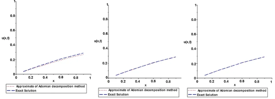
[image:6.595.55.542.92.492.2]

1.0

Figure 1. The exact solution and the approximate solution using ADM for ϕ ϕ ϕ3, ,5 10 at t=0.5 and 0≤ ≤x 1.

[image:6.595.59.538.531.704.2]

(7)

Example 2

Consider the nonlinear inhomogeneous wave equation

2 2 2_, _0,

tt xx

u u− − +u u = +xt x t t>

with specified initial conditions u x

( )

,0 1,= u xt

( )

,0 =x, and the boundary

con-ditions u

( )

0,t =1,ux

( )

0,t =t. Rewriting the wave equation in the operator form

as

2 2 2_.

tt xx

L u L u u u− − + = +xt x t

To solve initial-boundary value problem, firstly, we consider the t partial

solu-tion as 2 2 2

tt xx

L u L u u u= + − + +xt x t . Applying the inverse operator 1

tt

0 0d d t t tt

L− ₌ t t

∫ ∫

, gives

( )

_,

( )

_,0

( )

_,0 1

(

2 2

)

1

( )

_, 1 1 2

t tt tt xx tt tt

u x t ₌u x ₊tu x ₊L xt x t− ₊ ₊L L u x t− ₊L u L u− ₋ − _.

This introduces the recursive relations

( )

1

(

2 2

)

0 ,0 t ,0 tt

u ₌u x ₊tu x ₊L xt x t− ₊

1 1 1

1 , 0.

n tt xx n tt n tt n

u L L u− L u− L A n−

+ = + − ≥

where the nonlinear term _u2_{can be expressed by an infinite series of the} Adomian polynomials An given by:

( )

2

0 0 ,

A = u

1 2 0 1,

A = u u

( )

2

2 1 2 0 2,

A = u + u u

3 2 1 2 2 0 3,

A = u u + u u

( )

2

4 2 2 1 3 2 0 4,

A = u + u u + u u



So that first two terms are

3 2 4

0 1 1 1 ,

6 12

u = + +xt xt + x t

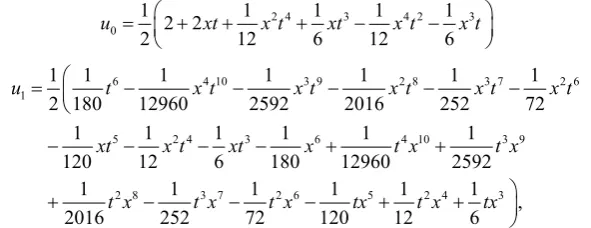
6 4 10 3 9 2 8 3 7

1

2 6 5 2 4 3

1 1 1 1 1

180 12960 2529 2016 252

1 1 1 1 _,

72 120 12 6

u t x t x t x t x t

x t xt x t xt

= − − − −

− − − −

Secondly, we consider the x partial solution 2 2 2

xx tt

L u L u u u= − + − −xt x t . Applying the inverse operator 1

xx

L− ₌ x x_′

∫ ∫

, gives

( )

_, 1

(

2 2

)

1

( )

_, 1

( )

_, 1 2

( )

_{, ,}

x xx xx tt xx xx

u x t _{= Φ +}L− _{− −}xt x t ₊L L u x t− ₋L u x t− ₊L u x t−

This gives the recursive relations

(

)

1 2 2

0 x,0 xx ,

u _{= Φ +}L− _{− −}xt x t

1 1 1

1 , , 0.

n x n xx tt n xx n xx n

u L L u− L u− L A n−

+ = Φ + − + ≥

(8)

( )

(

)

( )

1 2 2

0 1,0 2,0

4 2 3

1,0 2,0 ₁₂1 1₆ ,

xx

u c t c t x L xt x t

c t c t x x t x t

−

= + + − −

= + − −

The first approximant is ϕ =1 u0. Applying the x conditions to ϕ1 it is clear that c t1,0

( )

=1 and c2,0

( )

t =t. Thus, if the one-term approximant ϕ1 were

sufficient, thesolutionwould be 4 2 3

1 u0 1 xt ₁₂1 x t 1₆x t

ϕ

= = + − − . The next term

is

( )

1 1 1

1 1,1 2,1 xx tt 0 xx 0 xx 0.

u ₌c t ₊c t x L L u₊ − ₋L u− ₊L A−

Then ϕ = +2 u u0 1 is given by:

( )

6 4 10 3 9

2 1,1 2,1

2 8 3 7 2 6 5

1 1 1

1

180 12960 2592

1 1 1 1 _,

2016 252 72 120

xt c t c t x x t x t x

t x t x t x tx

ϕ = + + + − + +

+ − − −

Applying the condition at x=0_{, we have} c t_1,1

( )

=0_{. From the condition on} x at 0, we get c t2,1

( )

=0, thus

6 4 10 3 9 2 8

1

3 7 2 6 5 2 4 3

1 1 1 1

180 12960 2592 2016

1 1 1 1 1 _,

252 72 120 12 6

u x t x t x t x

t x t x tx t x tx

= − + + +

− − − + +

Next, we average the partial solutions, i.e. add two partial solutions and divide by two, so we obtain

2 4 3 4 2 3

0 1₂ 2 2 ₁₂1 1₆ ₁₂1 1₆

u = _ + xt+ x t + xt − x t − x t_

 

6 4 10 3 9 2 8 3 7 2 6

1

5 2 4 3 6 4 10 3 9

2 8 3 7 2 6 5 2 4 3

1 1 1 1 1 1 1

2 180 12960 2592 2016 252 72

1 1 1 1 1 1

120 12 6 180 12960 2592

1 1 1 1 1 1 _,

2016 252 72 120 12 6

u t x t x t x t x t x t

xt x t xt x t x t x

t x t x t x tx t x tx



= _ − − − − −



− − − − + +



+ − − − + + _



( )

0 ,

ap n

n

u ∞ u x t

=

∑

_{which is converge to the exact}

[image:8.595.224.520.421.535.2]

solution uex= +1 xt.

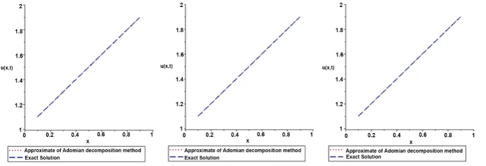
Table 2 shows the comparison between the absolute error of exact and ap-proximate solutions for various values of t. Figure 3 and Figure 4 give the plots for the exact solution and the approximate solution by application of (ADM) for

0.5, 1.0 t= t=

3. Modified Adomian Decomposition Method with Mixed

Conditions

(9)

[image:9.595.62.539.88.524.2]

Table 2.Absolute errors using ADM at t=0.5,t=1.0_and 0≤ ≤x 1_.

t = 1.0 t = 0.5

x

φ10

φ5

φ3

φ10

φ5

φ3

1.98867397e−13 1.94227703e−07

3.03130511e−04 7.38008938e−21

9.91381644e−11 1.16795669e−06

0.0

1.80979784e−14 5.24225154e−07

3.13576647e−04 1.32310675e−20

1.34624036e−10 1.11741220e−06

0.1

3.35618411e−13 8.92768322e−07

3.10560067e−04 1.87267309e−20

1.68442683e−10 1.02259378e−06

0.2

7.19015636e−13 1.27778455e−06

2.91108055e−04 2.27716130e−20

1.98929868e−10 9.15093801e−07

0.3

1.09372711e−12 1.64754249e−06

2.52542863e−04 2.45567197e−20

2.47291825e−10 1.07394957e−06

0.4

1.34001536e−12 1.95990772e−06

1.94233658e−04 1.54926759e−19

6.80058898e−10 2.78526691e−06

0.5

1.29712536e−12 2.16910519e−06

1.22320508e−04 1.31137692e−17

4.84484741e−09 1.02972732e−05

0.6

7.88380042e−13 2.27490316e−06

6.00678450e−05 6.42509911e−16

3.38038332e−08 3.49347643e−05

0.7

2.03620129e−13 2.54957010e−06

6.75505137e−05 1.89050311e−14

1.89000465e−07 1.02662323e−04

0.8

1.01270536e−12 4.36439340e−06

2.75330767e−04 3.75110306e−13

8.69375166e−07 2.66686450e−04

0.9

4.38984895e−11 1.27237836e−05

9.37415208e−04 5.43693717e−12

3.41245963e−06 6.26917478e−04

[image:9.595.60.541.90.517.2]

1.0

Figure 3.The exact solution and the approximate solution using ADM for ϕ ϕ ϕ3, ,5 10 at t=0.5.

[image:9.595.62.546.542.707.2]

(10)

term u0 can be set as function f and divided it into two parts, namely f1 and f2.

Under this assumption, we set f = +f1 f2. Also, based on this, we propose a slight variation only on the components u0 and u1, the variation is that only the

part f1 is assigned to the zeroth component u0, whereas the remaining part f2 is

combined with the other terms to define u1. This reduction in the number of

terms of u0 will result in reduction of the computational work and will accelerate

the convergence. Further, this slight variation in the definition of the compo-nents u0 and u1 may provide the solution by using two iterations only.

Further-more, the calculations below will show that sometimes there is no need to eva-luate the so-called Adomian polynomials required for the nonlinear differential equations. An important observation that can be made here is that the success of this method depends mainly on the proper choice of the parts f1 and f2. We have

been unable to establish any criterion to judge what forms of f1 and f2 can be

as-sumed to yield the acceleration demanded. It appears that trials are the only cri-teria that can be applied so far.

3.1. Boundary Value Problems

Based on the recurrence relation in Equation (2.8)

( )

1

0 x,0 xx , ,

u _{= Φ +}L g x t−

1 1

1 , 1 , 0.

u L L u− L A n−

+ = Φ + − − ≥

We can set 1

( )

0 x,0 xx ,

u _{= Φ +}L g x t− ₌ f _{, then we divide it into two parts, so that}

we formulate the modified recursive algorithm as follows:

0 1,

u = f

1 1

1 2 x,1 xx tt 0 xx 0,

u ₌ f _{+ Φ −}L L u− ₋L A−

1 1

1 , 1 , 1.

u L L u− L A n−

+ = Φ + − − ≥ (3.1)

Comparing the recursive scheme in Equation (2.8) of the ADM with the scheme in Equation (3.1) of the modified technique leads to the conclusion that in Equation (2.8) the zeroth component was defined by the function f, whereas in Equation (3.1), the zeroth component u0 was defined by only a part f1 of f, the

remaining part f2 of f is added to the definition of the component u1 in (3.1).

3.2. An alternative Combination of the Initial and Boundary

Conditions

Based on the recurrence relation in Equation (2.13), we can set

( )

(

1 1

)

0 1₂ ,0 t ,0 x,0 tt , xx ,

u ₌ u x ₊tu x _{+ Φ +}L g x t− ₊L g x t− ₌ f

Then we divide it into two parts, so that we formulate the modified recursive algorithm as follows:

0 1,

u = f

(

1 1 1 1

)

1 2 1₂ x,1 tt xx 0 xx tt 0 tt 0 xx 0 ,

(11)

(

1 1 1 1

)

1 1₂ , 1 , 1.

n x n tt xx n xx tt n tt n xx n

u L L u− L L u− L A L A− − n

+ = Φ + − − − − ≥ (3.2)

Comparing the recursive scheme in Equation. (2.13) of the ADM with the re-cursive scheme in Equation (3.2) of the modified technique leads to the conclu-sion that in (2.13) the zeroth component was defined by the function f, whereas in (3.2), the zeroth component u0 is defined only by a part f1 of f, the remaining

part f2 of f is added to the definition of the component u1 in (2.13).

In order to demonstrate the efficiency and applicability of the proposed me-thod, we study example of nonlinear partial differential equations here.

3.3. Numerical Experiments

Example 3

Consider the nonlinear inhomogeneous heat equation

2 2 2 _, _0,

t xx

u u= +u −x t +x t>

with specified conditions u x

( )

,0 =0, 0,u

( )

t =0,ux

( )

0,t =t.

Rewriting the heat equation in the operator form as

2 2 2 _.

t xx

L u L u u= + −x t +x

xx

L− ₌

_{∫ ∫}

x x_′_{, we get}

( )

_, 1

(

2 2

)

1

( )

_, 1 2

( )

_{, ,}

x xx xx t xx

u x t _{= Φ +}L x t− ₋x ₊L L u x t− ₋L u x t−

This gives the recursive relations

(

)

1 2 2

0 x,0 xx ,

u _{= Φ +}L x t− ₋x

1 1

1 , 1 , 0.

n x n xx t n xx n

u L L u− L A n−

+ = Φ + + − ≥

So that

( )

(

)

( )

1 2 2

0 1,0 2,0

4 2 3

1,0 2,0 ₁₂1 1 ,₆

xx

u c t c t x L x t x

c t c t x x t x

−

= + + −

The first approximant is ϕ =1 u0 Applying the x conditions to ϕ1 it is clear that c t1,0

( )

=0 and c t2,0

( )

=t. Thus, if the one-term approximant ϕ1 were

sufficient, the “solution” will be 4 2 3

1 0 1 1

12 6

u xt x t x

ϕ

= = + − _{. We set}u₀= f _,

then we divide it into two parts, so that

0 1 ,

u = f =xt

( )

1 1

1 2 1,1 2,1 0 0

4 2 3 1 1

1,1 2,1 0 0

1 1 _.

12 6

xx t xx

u f c t c t x L L u L A

x t x c t c t x L L u L A

− −

= + + + −

 

=_ − _+ + + −

 

Then ϕ = +2 u u0 1 is given by:

( )

4 2 3 1 1

2 xt ₁₂1 x t 1₆x c t c t x L L u L A1,1 2,1 xx t 0 xx 0

ϕ

_{= +} ₋ ₊ ₊ ₊ − ₋ −

(12)

DOI: 10.4236/ajcm.2018.82012 164 American Journal of Computational Mathematics x at 0, we get c t2,1

( )

=0, thus u1=0, and un+1=0,n≥1. Thus, the approx-imate solution is u u= 0=xt, which is the exact solution.

4. Improvement of the Inverse Operator with Mixed

Boundary Conditions

In 1999, Lesnic and Elliott [30] employed ADM for solving some inverse boun-dary value problems in heat conduction, also they applied the modification me-thod to deal with noisy input data and obtain a stable approximate solution. In

[32] Lesnic investigated the application of the decomposition method involving computational algebra for solving more complicated problems with Dirichlet, Neumann or mixed boundary conditions. In [30] the authors defined the

opera-tor 1

t

L− _{and as definite integrals given by}

0

1 1

0d , d 1 d

t x x

t x _x

L− ₌

_∫

t L_′ − ₌

_∫

x_′

_∫

′ x_′′_(4.1)

to solve the linear homogeneous heat equation u u xt = xx, 0< <x 1,t>0, subject to the mixed boundary conditions u x t

(

0,

)

=h t u1

( ) ( )

, x 1,t =h t2

( )

.

We will make an extension to the inverse operator (4.1) given in [30] to all cases of problems, so that we consider in this section, two types of problems: boundary value problems and initial-boundary value problems.

4.1. Boundary Value Problems

Consider Equations. (2.2)-(2.3), and applying the inverse operator 1 xx

L− _defined

by

1 x_d x_d

xx _a _b

L− ₌ x_′ ′ x_′′

∫

to both sides of Equation (2.4), gives

( )

_,

( ) (

_,

) ( )

, 1

( )

_, 1

( )

_, 1

( )

_,

xx xx tt xx

u b t

u x t u a t x a L g x t L L u x t L Nu x t x

− − −

∂

= + − + − −

∂ (4.2)

i.e. the boundary conditions can be used directly to solve the boundary value problem in x-direction.

Substituting

( )

0

, n ,

n

u x t ∞ u x t

=

∑

_{, and}

( )

(

₀ ₁ ₂

)

0

, n , , , , n

n

=

∑

_ _into

Equation (4.2), gives

( )

( ) (

) ( )

( )

1 0

1 1

0 0

,

, , ,

, ,

n xx

n

xx tt n xx n

n n

u b t

u x t u a t x a L g x t x

L L u x t L A x t

∞

−

=

∞ ∞

− −

= =

∂

= + − +

∂

− −

∑

This yields the recursive relations

( ) (

) ( )

1

( )

0

,

, xx , ,

u b t

u u a t x a L g x t x

−

∂

= + − +

∂

1 1

1 , 0.

n xx tt n xx n

u L L u− L A n−

+ = − − ≥ (4.3)

4.2. An Alternative Combination of the Initial and Boundary

Conditions

(13)

partial solution as in Equation (4.2) to get

( )

( ) (

) ( )

( )

1 1 1 1

1 1

, 1

, ,0 ,0 ,

2

, , , ,

, ,

t

tt xx tt xx xx tt

tt xx

u b t u x t u x u x t u a t x a

x L g x t L g x t L L u x t L L u x t L Nu x t L Nu x t

− − − − − − ∂  = _ + + + − ∂  + + − −  − − _  (4.4)

Substituting

( )

0

, n ,

n

u x t ∞ u x t

=

∑

_{, and}

( )

(

₀ ₁ ₂

)

0

, n , , , , n

n

=

∑

_ _into

Equation (4.3), gives

( )

( ) (

) ( )

( )

0

1 1 1

0

1 1 1

0 0 0

, 1

, ,0 ,0 ,

2

, , ,

n t

n

tt xx tt xx n

n

xx tt n tt n xx n

n n n

u b t u x t u x u x t u a t x a

x L g x t L g x t L L u x t

L L u x t L A x t L A x t

∞ = ∞ − − − = ∞ ∞ ∞ − − − = = = ∂  = _ + + + − ∂  + + −  − − − _ 

∑

so that the recurrence relations are

( )

( ) (

) ( )

1

( )

1

( )

0

,

1 _,0 _,0 _, _, _,

2 t tt xx

u b t

u u x u x t u a t x a L g x t L g x t x − − ∂   = _ + + + − + + _ ∂  

(

1 1 1 1

)

1 1₂ , 0.

n tt xx n xx tt n tt n xx n

u L L u− L L u− L A L A− − n

+ = − − − − ≥ (4.5)

To give a clear overview of these methods, we have chosen several differential equations. The examples will be approached by the Lesnic‘s Approach and the modified technique for comparison reasons. We also compare the approximate solution with the exact solution.

4.3. Numerical Experiments

Example 4

0, 0 1, 0,

t xx

u u− = ≤ ≤x t>

with specified conditions

( )

_,0 _{e , 0,}x

( )

_{e ,}t

( )

_1, _e1t x

u x ₌ u t ₌ u t ₌ + _.

Rewriting the heat equation in the operator form as L u L ut = xx . Applying the inverse operator 1

xx

0d 1 d

x x

xx

L− ₌ x_′ ′ x_′′

∫

, we get the recursive

rela-tions

( )

0

1,

0, u t ,

u u t x x

∂

= +

∂

1

1 , 0.

n xx t n

u L L u n−

+ = ≥

So that

1

0 et e ,t

u _{= +}x +

1 3 2 1

1 1₆e t 1₂et et 1₂e ,t

(14)

1 5 4 1 3 1

2 ₁₂₀1 e t ₂₄1 et 1 1_{3 2} et ₄1e t ₂₄5 e t ₃1e ,t

u ₌ +x ₊ x ₊ − ₋ + x ₊ x + ₊ x

 

 

( )

0 ,

ap n

n

u ∞ u x t

=

∑

solution ex t

ex

u ₌ + _.

Table 3 shows the comparison between the absolute error of exact and ap-proximate solutions for various values of t. Figure 5 and Figure 6 show the re-sults for the exact solution and the approximate solution by application of Les-nic’s approach for t=0.5, 1.0t= .

Example 5

, 0,

t xx

u u= +u t> with specified conditions u

( )

0,t e

( )

1π2t,ux

( )

0,t 0

−

= = _.

Rewriting the heat equation in the operator form a L u L u ut = xx + . Applying the inverse operator 1

xx

0d 1 d

x x

xx

L− ₌ x_′ ′ x_′′

∫

, we get the

recursive relations

( )

0 0, 0, ,

u t u u t x

x

∂

= +

∂

1 1

1 , 0.

n xx t n xx n

u L L u− L u n−

+ = − ≥

So that

( )

₁_π2

0 e ,

t

u = −

(

)

( )

₁_π2

( )

_{1 π}2

2

1 1 1₂ π2 e e ,

t t

u = _ − − − − _x

 

(

)

₂

( )

_π2

(

)

( )

_π2

( )

_π2

2 1 2 1 1 4

2 1 1_{4 6} 1 π e 1₃ 1 π e 1₆e ,

t t t

u = _ − − − − − − _x

 + 

Continuing in a similar way u u3, , ,4  un are obtained for some n, then we

( )

0 ,

ap n

n

u ∞ u x t

=

∑

which converged to the exact

solution uex e

( )

1π2tcos

( )

πx

−

= .

Table 4 shows the comparison between the absolute error of exact and ap-proximate solutions for various values of t. Figure 7 and Figure 8 show the re-sults for the exact solution and the approximate solution by application of Les-ni’s approach for t=0.5, 1.0t= _.

Example 6

Consider the nonlinear inhomogeneous wave equation

2 ₂ 2 ₂ 2 4 4_, _0,

tt xx

u u− +u = x − t +x t t>

with specified initial condition u x

( )

,0 =0,u xt

( )

,0 =0 and the boundary

con-ditions u

( )

0,t =0,ux

( )

0,t =0.

Rewriting the wave equation in the operator form as

2 ₂ 2 ₂ 2 4 4_.

tt xx

(15)

[image:15.595.58.547.91.295.2]

Table 3. Absolute errors of Lesnic’s approach at t=0.5,t=1.0_.

t = 1.0 t = 0.5

[image:15.595.57.542.326.706.2]

x φ10 φ5 φ3 φ10 φ5 φ3 0.00000000e+00 0.00000000e+00 0.00000000e+00 0.00000000e+00 0.00000000e+00 0.00000000e+00 0.0 1.25782220e−04 1.15032229e−02 7.00545484e−02 7.62907729e−05 6.97705740e−03 4.24902315e−02 0.1 2.48467264e−04 2.27231903e−02 1.38378497e−01 1.50703014e−04 1.37823116e−02 8.39308011e−02 0.2 3.65034220e−04 3.33836232e−02 2.03286055e−01 2.21404446e−04 2.02481910e−02 1.23299225e−01 0.3 4.72612822e−04 4.32220236e−02 2.63178475e−01 2.86654167e−04 2.62154825e−02 1.59625814e−01 0.4 5.68554127e−04 5.19961385e−02 3.16582967e−01 3.44845510e−04 3.15372522e−02 1.92017276e−01 0.5 6.50495743e−04 5.94899244e−02 3.62187938e−01 3.94545612e−04 3.60824631e−02 2.19678089e−01 0.6 7.16419995e−04 6.55188663e−02 3.98874156e−01 4.34530692e−04 3.97392012e−02 2.41929405e−01 0.7 7.64703609e−04 6.99345194e−02 4.25741433e−01 4.63816184e−04 4.24174302e−02 2.58225232e−01 0.8 7.94157682e−04 7.26281622e−02 4.42130336e−01 4.81680983e−04 4.40512072e−02 2.68165604e−01 0.9 8.04056958e−04 7.35334732e−02 4.47638409e−01 4.87685197e−04 4.46003060e−02 2.71506419e−01 1.0

Table 4. Absolute errors of Lesnic’s approach at t=0.5,t=1.0.

t = 1.0 t = 0.5

x φ10 φ5 φ3 φ10 φ5 φ3 0.00000000e+00 0.00000000e+00 0.00000000e+00 0.00000000e+00 0.00000000e+00 0.00000000e+00 0.0 4.00000000e−33 3.62569093e−16 1.87405030e−10 4.00000000e−31 3.05774246e−14 1.58048860e−08 0.1 5.30984100e−27 3.70439590e−13 1.19307420e−08 4.47807730e−25 3.12411864e−11 1.00618440e−06 0.2 1.76377518e−23 2.12818773e−11 1.34709647e−07 1.48748759e−21 1.79481652e−09 1.13607976e−05 0.3 5.55353720e−21 3.75953232e−10 7.47656780e−07 4.68360013e−19 3.17061819e−08 6.30539648e−05 0.4 4.80770055e−19 3.47801646e−09 2.80759946e−06 4.05459549e−17 2.93320054e−07 2.36780141e−04 0.5 1.83884976e−17 2.13603726e−08 8.22461404e−06 1.55080207e−15 1.80143646e−06 6.93626458e−04 0.6 4.00205716e−16 9.88361203e−08 2.02783311e−05 3.37515258e−14 8.33538786e−06 1.71018201e−03 0.7 5.76423702e−15 3.71583868e−07 4.40342408e−05 4.86129475e−13 3.13376896e−05 3.71364715e−03 0.8 6.05663528e−14 1.19178044e−06 8.67192471e−05 5.10789012e−12 1.00509330e−04 7.31350601e−03 0.9 4.96182279e−13 3.37123368e−06 1.58019709e−04 4.18457517e−11 2.84314481e−04 1.33266620e−02 1.0

[image:15.595.58.542.332.693.2]

(16)

[image:16.595.63.541.74.242.2]

[image:16.595.61.543.281.441.2]

Figure 6.The exact solution and the approximate solution of Lesnic’s approach for ϕ ϕ ϕ3, ,5 10 at t=1.0.

Firstly, we consider the t partial solution as

2 ₂ 2 ₂ 2 4 4_.

tt xx

L u L u u= − + x − t +x t

Applying the inverse operator 1 tt

0 0d d t t tt

L− ₌ t t

∫ ∫

, gives the

[image:16.595.64.536.475.623.2]

(17)

( )

1

(

2 2 4 4

)

0 ,0 t ,0 tt 2 2 ,

u ₌u x ₊tu x ₊L− x ₋ t ₊x t

1 1

1 , 0.

n tt xx n tt n

u L L u− L A n−

+ = − ≥

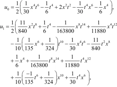
So that

4 6 4 2 2

0 ₃₀1 1₆ ,

u = x t − t +x t

2 8 4 8 14 4 12

1

6 10 4 6

11 1 1 1

840 6 163800 11880

1 1 1 1 _,

10 135 324 30

u x t t x t x t

x t x t

= + − +

 

− _ + _ −

 

Secondly, we consider the x partial solution

2 ₂ 2 ₂ 2 4 4_.

xx tt

L u L u u= + − x + t −x t

0d 0 d

x x

xx

L− ₌ x_′ ′ x_′′

∫

, gives the

recursive relations

( )

1

(

2 2 4 4

)

0 0, 0, xx 2 2 ,

u t

u u t x L x t x t x

−

∂

= + + − + −

∂

1 1

1 , 0.

n xx t n xx n

u L L u− L A n−

+ = − ≥

So that

4 6 4 2 2

0 ₃₀1 1₆ ,

u = − t x − x +x t

2 8 4 8 14 4 12

1

6 10 4 6

11 1 1 1

840 6 163800 11880

1 1 1 1 _,

10 135 324 30

u t x x t x t x

t x t x

= − + + +

−

 

+ _ + _ +

 

Next, we average the partial solutions, i.e. add two partial solutions and divide by two, so we obtain

4 6 4 2 2 4 6 4

0 1 1_{2 30} 1₆ 2 ₃₀1 1₆ ,

u = _ x t − t + x t − t x − x _

 

2 8 4 8 14 4 12

1

6 10 4 6 2 8

4 8 14 4 12

6 10 4 6

1 11 1 1 1

2 840 6 163800 11880

1 1 1 1 11

10 135 324 30 840

1 1 1

6 163800 11880

1 1 1 1 _,

10 135 324 30

u x t t x t x t

x t x t t x

x t x t x

t x t x



= _ + − +



 

− _ + _ − −

 

+ + +

− 

 

+ _ + _ + _

  

( )

0 ,

ap n

n

u ∞ u x t

=

∑

solution 2 2

ex

[image:17.595.271.472.498.648.2]

u =x t _.

(18)

[image:18.595.62.537.89.507.2]

Table 5. Absolute errors of Lesnic’s approach at t=0.5,t=1.0.

t = 1.0 t = 0.5

x

φ10

φ5

φ3

φ10

φ5

φ3

1.17411886e−14 6.66358850e−07

2.99609298e−04 6.85095911e−25

1.01879027e−11 2.92793246e−07

0.0

6.46368619e−15 6.67335460e−07

2.99751384e−04 5.49993680e−25

1.01884440e−11 2.92797760e−07

0.1

9.47122029e−15 6.68628865e−07

2.99906957e−04 4.25441720e−24

1.01838277e−11 2.92714604e−07

0.2

3.60495597e−14 6.65318536e−07

2.99261398e−04 1.04069553e−23

1.01582155e−11 2.90660076e−07

0.3

7.21721640e−14 6.49193205e−07

2.96428943e−04 1.88856065e−23

1.03640472e−11 2.59880611e−07

0.4

1.14059558e−13 6.08842328e−07

2.89265750e−04 1.39263400e−24

2.03770775e−11 6.38490216e−09

0.5

1.53190969e−13 5.30208113e−07

2.73991554e−04 1.04956960e−20

2.05585573e−10 1.55441030e−06

0.6

1.74249490e−13 4.00247226e−07

2.42057261e−04 1.45619577e−18

2.34523011e−09 8.35705522e−06

0.7

1.53300820e−13 2.32477815e−07

1.70952966e−04 1.03741414e−16

2.00278856e−08 3.27155910e−05

0.8

2.08420940e−14 2.20560700e−07

8.65289576e−07 4.44838968e−15

1.33275317e−07 1.07359772e−04

0.9

1.53639602e−12 1.50572369e−06

4.18259832e−04 1.27588322e−13

7.26354463e−07 3.09754605e−04

1.0

[image:18.595.59.538.90.515.2]

[image:18.595.62.550.533.701.2]

(19)

results for the exact solution and the approximate solution by application of Lesnic’s approach for t =0.5,t =1.0.

Example 7

Consider the nonlinear inhomogeneous heat equation

2 2 2_ex _{e ,}x _0,

t xx

u u= +u u t− − + t>

with specified conditions u x

( )

,0 =0, 0,u

( )

t =t u, x

( )

0,t =t. Rewriting the heat

equation in the operator form as

2 2 2_ex _{e .}x

t xx

L u L u u u t= + − − + Applying the inverse operator 1

xx

0d 0d

x x

xx

L− ₌ x_′ ′ x_′′

∫

, we get the

recursive relations

( )

1

(

2 2

)

0

0,

0, e x e ,x

xx

u t

u u t x L t x

−

∂

= + + −

∂

1 1 1

1 , 0.

n xx t n xx n xx n

u L L u− L u− L A n−

+ = + − ≥

So that

2 2 2 2

0 1 1₄ 1₂ 1₄ e x e ,x

u = + + −t xt t − t x x+ + t −

We set u0= f then we divide it into two parts, so that

0 1 ,

u = f t xt= +

1 1 1

1 2 0 0 0

2 2 2 2 3 2

2 4 2 3 2 2 3 2

1 1 1 1 1

1 e e

4 2 4 6 2

1 1 1 1 1 _,

12 3 2 6 2

xx t xx xx

x x

u f L L u L u L A

t t x x t x x

t x t x t x tx tx

− − −

= + + −

 

= −_ − + + − _+ +

 

− − − + +

( )

0 ,

ap n

n

u ∞ u x t

=

∑

solution ex

ex

[image:19.595.200.540.103.566.2]

u =t .

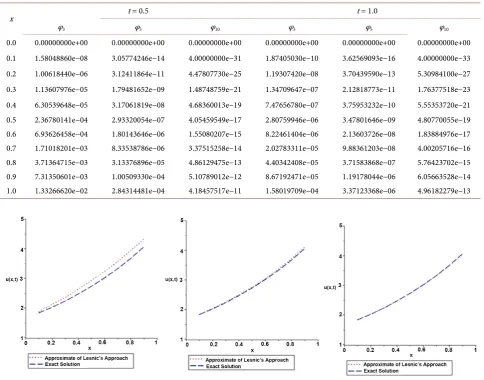
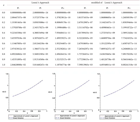
Table 6 shows the comparison between the absolute error of exact and ap-proximate solutions Lesnic’s approach and modified of Lesnic’s approach for various values of t. Figure 11 and Figure 12 show the results for the exact solu-tion and the approximate solusolu-tion by applicasolu-tion of Lesnic’s approach and mod-ified of Lesnic’s Approach for t=0.5_.

5. Conclusion

(20)

[image:20.595.56.540.90.513.2]

Table 6. Absolute errors of Lesnic’s approach and modified of Lesnic’s Approach at t=0.5.

modified of Lesnic’s Approach Lesnic’s Approach

x

φ10

φ5

φ3

φ10

φ5

φ3

1.00000000e−16 1.00000000e−27

0.00000000e+00 0.00000000e+00

2.00000000e−24 0.00000000e+00

0.0

1.24058539e−17 1.06888605e−16

3.81571653e−09 1.37823812e−10

3.57237376e−14 2.00447357e−08

0.1

1.83039464e−16 3.14421657e−13

2.67012987e−07 8.00849170e−11

3.85833086e−11 1.33381463e−06

0.2

5.19918722e−17 4.40980463e−11

3.31116702e−06 1.19984480e−11

2.34517027e−09 1.57920700e−05

0.3

2.58912426e−16 1.27255431e−09

2.01789433e−05 7.93648411e−11

4.38853494e−08 9.22165384e−05

0.4

7.73424325e−16 1.66889704e−08

8.32226565e−05 1.49935927e−10

4.30762657e−07 3.65597018e−04

0.5

1.65874377e−14 1.35122395e−07

2.67910691e−04 1.95254487e−10

2.81244230e−06 1.13467005e−03

0.6

4.24060812e−13 7.88954237e−07

7.26544297e−04 2.35238261e−10

1.38657115e−05 2.97453012e−03

0.7

7.09170229e−12 3.63635665e−06

1.73726451e−03 2.49626415e−10

5.56852385e−05 6.89226862e−03

0.8

8.56616462e−11 1.40126738e−05

3.77230615e−03 1.32152517e−09

1.91314569e−04 1.45351895e−02

0.9

8.00241318e−10 4.69348011e−05

7.59013963e−03 1.18704774e−08

5.81448247e−04 2.84628000e−02

1.0

[image:20.595.58.540.93.509.2]

[image:20.595.62.534.540.705.2]

(21)

The accuracy and computational efficiency of the proposed method are verified by numerical examples. Thus, the method is highly recommended for varieties of mixed boundary value problems.

References

[1] Carslaw, H.S. and Jaeger, J.C. (1948) Conduction of Heat in Solids. Clarendon Press, Oxford.

[2] Carrier, G.F., Krook, M. and Pearson, C.E. (1966) Functions of a Complex Variable. McGraw-Hill, New York.

[3] Courant, R. and Hilbert, D. (1953) Methods of Mathematical Physics. Vol. 1, Inters-cience Publishers Inc., New York.

[4] Sneddon, I.N. (1966) Mixed Boundary Value Problems in Potential Theory. Wiley, New York.

[5] Tranter, C.J. (1951) Integral Transforms in Mathematical Physics. Wiley, New York.

[6] Fabrikant, V.I. (1991) Mixed Boundary Value Problems of Potential Theory and their Applications in Engineering. Kluwer, Boston.

[7] Sherwood, J.D. and Stone, H.A. (2001) Leakage through Filtercake into a Fluid Sampling Probe. Physics of Fluids, 13, 1151-1159.https://doi.org/10.1063/1.1360712

[8] Warrick, A.W., Broadbridge, P. and Lomen, D.O. (1992) Approximations for Diffu-sion from a Disc Source. Applied Mathematical Modelling, 16, 155-161.

https://doi.org/10.1016/0307-904X(92)90067-D

[9] He, J.H. (2008) An Elementary Introduction to the Homotopy Perturbation Me-thod. Computers & Mathematics with Applications, 57, 410-412.

https://doi.org/10.1016/j.camwa.2008.06.003

[10] Wazwaz, A.M. (2006) The Modified Decomposition Method for Analytic Treat-ment of Differential Equations. Applied Mathematics and Computation, 173, 165-176.https://doi.org/10.1016/j.amc.2005.02.048

[11] Duan, J.S. and Rach, R. (2011) A New Modification of the Adomian Decomposition Method for Solving Boundary Value Problems for Higher Order Nonlinear Diffe-rential Equations. Applied Mathematics and Computation, 218, 4090-4118.

https://doi.org/10.1016/j.amc.2011.09.037

[12] Adomian, G. and Rach, R. (1983) Inversion of Nonlinear Stochastic Operators.

Journal of Mathematical Analysis and Applications, 91, 39-46.

https://doi.org/10.1016/0022-247X(83)90090-2

[13] Adomian, G. (1986) Nonlinear Stochastic Operator Equations. Academic, Orlando. [14] Adomian, G. (1989) Nonlinear Stochastic Systems Theory and Applications to

Physics. Kluwer Academic, Dordrecht.https://doi.org/10.1007/978-94-009-2569-4

[15] Adomian, G., Rach, R. and Meyers, R. (1991) An Efficient Methodology for the Physical Sciences. Kybernetes, 20, 24-34.https://doi.org/10.1108/eb005909

[16] Adomian, G. and Rach, R. (1993) Analytic Solution of Nonlinear Boundary Value Problems in Several Dimensions by Decomposition. Journal of Mathematical Anal-ysis and Applications, 174, 118-137. https://doi.org/10.1006/jmaa.1993.1105 [17] Adomian, G. and Rach, R. (1993) A New Algorithm for Matching Boundary

Condi-tions in Decomposition SoluCondi-tions. Applied Mathematics and Computation, 57, 61-68.https://doi.org/10.1016/0096-3003(93)90012-4

(22)

DOI: 10.4236/ajcm.2018.82012 174 American Journal of Computational Mathematics Nonlinear Boundary-Value Problems. Nonlinear Analysis, 23, 615-619.

https://doi.org/10.1016/0362-546X(94)90240-2

[19] Adomian, G. (1994) Solving Frontier Problems of Physics: The Decomposition Method. Kluwer Academic, Dordrecht.https://doi.org/10.1007/978-94-015-8289-6 [20] Wazwaz, A.M. (2000) Approximate Solutions to Boundary Value Problems of

Higher Order by the Modified Decomposition Method. Computers & Mathematics with Applications, 40, 679-691.https://doi.org/10.1016/S0898-1221(00)00187-5

[21] Wazwaz, A.M. (2000) The Modified Adomian Decomposition Method for Solving Linear and Nonlinear Boundary Value Problems of 10th-Order and 12th-Order.

International Journal of Nonlinear Sciences and Numerical Simulation, 1, 17-24.

https://doi.org/10.1515/IJNSNS.2000.1.1.17

[22] Wazwaz, A.M. (2001) A Reliable Algorithm for Obtaining Positive Solutions for Nonlinear Boundary Value Problems. Computers & Mathematics with Applica-tions, 41, 1237-1244.https://doi.org/10.1016/S0898-1221(01)00094-3

[23] Wazwaz, A.M. (2001) The Numerical Solution of Fifth-Order Boundary Value Problems by the Decomposition Method. Journal of Computational and Applied Mathematics, 136, 259-270.https://doi.org/10.1016/S0377-0427(00)00618-X

[24] Wazwaz, A.M. (2001) The Numerical Solution of Sixth-Order Boundary Value Problems by the Modified Decomposition Method. Applied Mathematics and Computation, 118, 311-325.https://doi.org/10.1016/S0096-3003(99)00224-6

[25] Wazwaz, A.M. (2001) A Reliable Algorithm for Solving Boundary Value Problems for Higher-Order Integro-Differential Equations. Applied Mathematics and Com-putation, 118, 327-342.https://doi.org/10.1016/S0096-3003(99)00225-8

[26] Wazwaz, A.M. (2002) The Numerical Solution of Special Fourth-Order Boundary Value Problems by the Modified Decomposition Method. International Journal of Computer Mathematics, 79, 345-356.https://doi.org/10.1080/00207160211928

[27] Jang, B. (2008) Two-Point Boundary Value Problems by the Extended Adomian Decomposition Method. Journal of Computational and Applied Mathematics, 219, 253-262.https://doi.org/10.1016/j.cam.2007.07.036

[28] Ebaid, A.E. (2010) Exact Solutions for a Class of Nonlinear Singular Two-Point Boundary Value Problems: The Decomposition Method. Zeitschrift für Naturfor-schung, 65a, 1-6.https://doi.org/10.1515/zna-2010-0301

[29] Adomian, G. (1986) A New Approach to the Heat Equation—An Application of the Decomposition Method. Journal of Mathematical Analysis and Applications, 113, 202-209.https://doi.org/10.1016/0022-247X(86)90344-6

[30] Lesnic, D. and Elliott, L. (1999) The Decomposition Approach to Inverse Heat Conduction. Journal of Mathematical Analysis and Applications, 232, 82-98.

https://doi.org/10.1006/jmaa.1998.6243

[31] Wazwaz, A.M. (1999) A Reliable Modification of Adomian’s Decomposition Me-thod. Applied Mathematics and Computation, 102, 77-86.

https://doi.org/10.1016/S0096-3003(98)10024-3