Inclusion of Efficient Rules in PRISM Algorithm for Data
Classification
Yogesh Wanjari
Assistant professor Dept. of CSE, WCEM Nagpur-441108, IndiaSanjay Nagpure
Dept. of CSE, WCEM Nagpur-441108, IndiaGokul Chute
Dept. of CSE, WCEM Nagpur-441108, IndiaYogeshwari Kamble
Dept. of CSE, WCEM Nagpur-441108, IndiaABSTRACT
Data classification is the process of classify data into different types, forms or any other separate classes. Data may be classified for a different of reasons, including ease of access, to observe with regulatory requirements, and to meet various other business or personal intention. In some cases, data classification is a regulatory requirement, as data must be searchable and recoverable within specified time durations. the focus of this paper is on the description of rule based classification and ensemble learning as well as the discussion on some existing methods and techniques. In our proposed approach we are using PRISM algorithm for rule induction. Based on induced rule, test data will be classified. In this paper we proposed Maximized the classification accuracy, Minimize the error rate and also Minimize the classification time. After that experimental evaluation will be performed with basic PRISM algorithm and will show comparative analysis of basic PRISM algorithm and other data classification algorithm such as SVM, Decision Tree, Perceptron Model and Logistic Regression. After comparing these classification algorithms, we found that Maximum accuracy using PRISM algorithm.
General Terms
Classification, Machine Learning, Confusion Matrix and Algorithms.
Keywords
Machine learning, Supervised Machine Learning, Classification, Confusion Matrix.
1.
INTRODUCTION
Machine learning is one of the fastest growing areas of computer science, with far-reaching applications. machine learning algorithms can be used for two main purposes in data classification processes and algorithms [20]. First one is to build a predictive model which is used to make predictions according to given data and the other one is to discover some meaningful and useful knowledge from classified dataset [13]. Machine learning is a branch of artificial intelligence and contains two stages: training and testing. Training is aims to learn something from well-known properties by using learning algorithms and somewhere testing aims to makes predictions on unknown properties by using the knowledge learned in training stage. In practice, a machine learning task normally aims to build a model that is further used to make predictions by taking possession of learning algorithms. That’s why this task is usually referred to as predictive impersonation. According to ACPRISM Machine Learning is the field of study that gives computers the ability to learn
attribute of numbers, belongs to some specific class. Decision Tree Analysis is a general, predictive modelling tool that has applications spanning a number of different region. decision trees are constructed via an algorithmic approach that identifies ways to split a data set based on different conditions and parameters [18].
2.
LITERATURE SURVEY
In this section we have reviewed some different papers to get information about the existing work and rule induction algorithm would be helpful. Cendrowska, J. studied the problems on Quinlan’s ID3 algorithm where some major limitations to the ID3 algorithm had been identified by author which makes its use unsuitable for many domains [1]. So to reduced such problems author describes a new algorithm, called PRISM which, although based on ID3, uses a different induction strategy to induce rules which are modular, thus many of the problems associated with decision trees are avoid. PRISM is totally rule based algorithm it takes as input a training set entered as a file of ordered sets of attribute values, each set being terminated by a classification. Information about the attributes and classifications is input from a separate file at the start of the program, and the results are output as individual rules for each of the classifications listed in terms of the described quality. When the new induction algorithm PRISM where proposed it describes some of the result obtained by applying it to different training sets [1]. Hadi, W.E et al. introduced an efficient AC algorithm called ACPRISM which is based on the PRISM algorithm framework. in their proposed work author mainly focuses on an integration between associations rules and classification tasks that aim to predict unseen samples. The main reason behind the integration of classification and association rule are, the high predictive accuracy of resulting algorithms and The resulting algorithms produces more understandable rules, they said the AC algorithms produce and gives more accurate results as compare to classical data mining algorithms. They give the comparative analysis between ACPRISM algorithm and some other well-known algorithms. The ACPRISM algorithm integrates three different approaches together, namely divide-and-conquer strategy, covering approach, and Associate classification. The authors doing their experiments on 16 different datasets [2]. Another AC algorithm called Fast Associative Classification Algorithm. they investigate their proposed algorithm against other AC algorithms. Their proposed approach based on AC mining which is a new branch of data mining and machine learning that classifies unseen instance based on association rules [3]. They mark that AC mining approach is widely used for a number of reasons. First, it produces higher classification accuracy rates for the outputting classifier than other data mining and machine learning approaches. Second, rules produced by AC mining classifier are simple and illustrated by simple “if-then” rules. In this paper the primary goal of AC mining approach is to build a model from huge database training data to predict the type of unseen testing data. Hadi, W.E et al. proposed algorithm works on the concept of vertical mining approach called Diffset [4]. This approach had gone through three steps
[image:2.595.304.553.96.462.2]
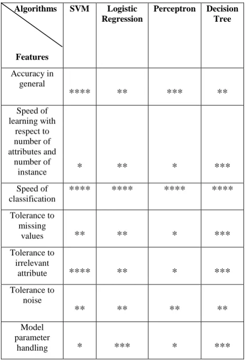
Table 1: Comparing learning algorithms (****stars represents best and *star represent worst performance) Algorithms
Features
SVM Logistic Regression
Perceptron Decision Tree
Accuracy in general
****
**
***
**
Speed of learning with
respect to number of attributes and
number of
instance
*
**
*
***
Speed of
classification
****
****
****
****
Tolerance to missing
values
**
**
*
***
Tolerance to irrelevant
attribute
****
**
*
***
Tolerance to noise
**
**
**
**
Model parameter
[image:2.595.306.553.98.462.2]handling
*
***
*
***
finding the accuracy, tolerance to irrelevant attribute, speed of learning, tolerance to missing values and tolerance to noise. Perceptron can only classify linearly separable sets of attributes. If a straight line or plane can be drawn to separate the input instances into their correct categories, input instances are linearly separable and the perceptron will find the solution. If the instances are not linearly separable learning will never reach a point where all instances are classified properly [8]. Perceptron gives the best result for speed of classification whereas gives the worst result for learning speed, tolerance to missing value, tolerance to irrelevant attribute, and model parameter handling. It gives good result for accuracy. Decision Trees are trees that classify instances by sorting them based on feature values. Each node in a decision tree represents a feature in an instance to be classified, and each branch represents a value that the node can assume. Instances are classified starting at the root node and sorted based on their feature values [10]. Decision tree gives good result foe speed of learning, tolerance to missing value, tolerance to irrelevant attribute, and model parameter handling whereas gives best result for speed of classification. It gives worst result for accuracy in general and tolerance to noise. for artificial intelligence researcher on constructing knowledge based system [4]. such as Discovering all frequent rules, building the classifier i.e. model, and predicting a new unseen instance i.e. testing data. After the generations of all frequent rules the FACA algorithm analyzed their confidence value. They conducted their experiments on 17 machines with 16G main memory and using WEKA software environment. The Tzung-Pei explained that training instance in real application domains sometimes come in two-stage way, first an initial set of training data are collected by experts, teachers, users, books. Its amount is usually large. And at stage two this rules are modified by new training data. high dimensionality in phishing websites [3]. Tzung-Pei et al. here proposed the two-phase PRISM learning algorithms. The main idea of this proposed approach is to put effectiveness during solving the learning problems. The general learning concept of training instance had become completely important The PRISM learning algorithm has a good characteristic of decomposability, which makes it suitable for two-phase learning [4]. Bruni, R. et al. proposed their work on Effective classification using a small training set based on discretization and statistical analysis. their work deals with the problem of producing a fast and accurate data classification, learning it from a possibly small set of records that are already classified. proposed approached of this paper is based on the framework called Logical Analysis of Data (LAD) [5]. but raised with information obtained from statistical considerations on the data. Bruni, R. discussed how the number of discrete optimization problems are solved in the different steps of the procedure, but their computational demand can be controlled. Also here the accuracy of the proposed approach is compared to the standard Logical Analysis of Data algorithm, of Support Vector Machine [5]. Cunhe L. et al. proposed a new semi-supervised vector machine learning algorithm based on active learning. this algorithm mainly focuses on improving the performance of classifiers which is practically approach for classifying small number of labeled samples and a large number of unlabeled samples respectively. The semi-supervised learning which uses a small amount of labeled data to obtain an initial classifier. This proposed approach effectively overcome slow training speed and low training accuracy rate with the traditional TSVM algorithm [6]. In a classification rule, the resultant with a single output represents the class predicted and the predecessor with a single or multiple inputs represents the sufficient condition to have this
class predicted.
[image:3.595.313.542.79.389.2]3.
SYSTEM OVERVIEW
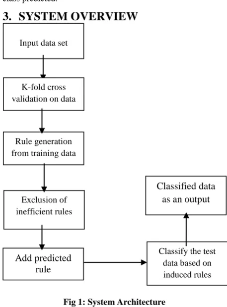
Fig 1: System Architecture
The system architecture flow is broadly divided into following components
3.1
Input data set
The input dataset for the system means we give the Training data to the system. In this system, we give the input in the form of any kind of dataset where the data is present in well-structured form. The classes, instances, and parameters are the basic part of the input dataset. Because of the well-structured dataset the system requires less time to perform the rest of the operations on the data.
3.2
K-Fold Cross validation of Training
data
The Cross Validation is a very important technique which is widely used in the field of data mining and machine learning. One type of cross validation is the K-Fold Cross Validation. Here suppose we use 10-Fold cross validation. In the 10-fold cross validation the data set is divided into 10 subsets, and the validation checking method repeated 10 times. Each time the one out of 10 subsets is used as test data and the other 9 subset put together as training data. Then the average error across all 10 trials is calculated. The advantage of this method is that every data point gets to be in a test set exactly once, and gets to be in a training set 9 times. The variance of the resulting evaluation is reduced as 10 is increased [17].
3.3
Rule generation
After the K-fold cross validation there are certain rules are generated from training subset. this model generate a set of rules based on the features of the data in the training dataset. Further these rules can be used for classification of future unknown data items. In order to generates a rule-based classifier we can follow a direct method to extract rules directly from data. The advantages of rule-based classifiers are that they are extremely expressive since they are symbolic
Input data set
Rule generation from training data
Exclusion of inefficient rules
Add predicted rule
Classify the test data based on induced rules Classified data
as an output K-fold cross
and operate with the attributes of the data without any variation. These rules are applicable for doing data classification of any dataset.
3.4
Exclusion of inefficient rules
In an exclusion of inefficient rules, we have to remove inefficient rule of rules from the generated rule set which does not satisfy the condition of dataset or gives wrong result for given dataset. This method helps to remove unwanted rule from training data set.
3.5
Add predicted rule
As a substitute of some rules which is excluded from rule set we add one default predicted rule. This rule which is correctly classify instance from data sets. This mean that it can describe the most common cases, but that it was not correct for all data in the training set. On the basis of most occurrence class in the dataset we generate default predicted rule for that class. Based on this induced rules we get some better results regarding to data classification.
3.6
Classify the test data based on induced
rules
We classify the test data based on induced rule method in this method we apply an individual rule for each classes. According to number of instances and attributes which present in classes we have to calculate confusion matrix. In Table 2 we describe confusion matrix it is classify into two types.
3.7
Classified data as an output
This is the final step where the output of the dataset generated in the form of graph which gives the easy identification to the Accuracy, error rate, and the classification time of the dataset. And give comparative analysis of the proposed approach as an output.
4.
ALGORITHM
Algorithm for classification //X=Feature _Name;
//Y=Class_Name;
//clf=Decision-Tree-Classifier;
//pred=Prediction of feature;
//f=Feature_Selection by Rules;
//cm=confusion_matrix;
1. Ruleset= {f};
2. Initialized X and Y;
3. Select the best Attribute X using the cm;
4 for each values X contain in Y
5. Initialize pred= clf.predict(X);
6.for each pred in X and Y;
7.Calculate pred;
8.end for;
9. end for;
10.if X==Y then
11.Correctly classify f;
12. else
13 reject X;
14. end if;
15. Evaluate test set of Y.
16. Correctly classify X and Y.
17. END
An algorithm of classification we are implement to classify from given data set of Animal species. Now, here we start actual data classification. The above algorithm provides details about how to classify the data from dataset and also measure the accuracy. We used Decision-Tree-Classifier, Prediction of feature, Feature Selection by Rules and confusion matrix to examine the result of classification.
First step we initialize rule set of feature f. in this step we initialize about 16 features namely hair, feathers, eggs, milk, airborne, aquatic, predator, toothed, backbone, breathes, venomous, fins, legs, and domestic etc.
In second step we initialize X and Y where X represent features of the Animals and Y represent the classes which is belongs from Animals.
In third step we use confusion matrix to select the best attribute from X.
In step number 4 we iteratively check features of X containing in class of Y.
In step number 5 we initialized prediction feature using decision tree classifier.
In step number 6 and 7 used to calculate prediction features which is present in X and Y.
In next step number 10 check the condition for correct classification for feature f is present or not.
In step number 15 we evaluate test data set of Y, which is examine after classification.
Finally, algorithm examine the correctly classify X and Y for our data set.
5.
EXPERIMENT
the data of 102 different animal species and separated it into 7 different classes named as Mammals, Bird, Reptile, Fish, Amphibian, Bug and Invertebrate. We classify this dataset on
the basis of 15 different parameters named as Hair, Feathers, Eggs, Milk, Airborne, Aquatic, Predator, Toothed, Backbone, Breathes, Venomous, Fins, Legs, Tail, and Domestic.
Table 1: Data set uses for Experiment Class
No.
No. of animal species in the
class Class Type Animal Names
1. 41 Mammals
aardvark, antelope, bear, boar, buffalo, calf, cavy, cheetah, deer, dolphin, elephant, fruitbat, giraffe, girl, goat, gorilla, hamster, hare, leopard, lion, lynx, mink, mole, mongoose, opossum, Oryx, platypus, polecat, pony, porpoise, puma, pussycat, raccoon,
reindeer, seal, sealion, squirrel, vampire, vole, wallaby, wolf
2. 20 Bird chicken, crow, dove, duck, flamingo, gull, hawk, kiwi, lark, ostrich, parakeet, penguin, pheasant, rhea, skimmer, scuba, sparrow, swan, vulture, wren
3. 5 Reptile pit viper, sea snake, slowworm, tortoise, tuatara
4. 13 Fish bass, carp, catfish, chub, dogfish, haddock, herring, pike, piranha, seahorse, sole, stingray, tuna
5. 4 Amphibian frog, frog, newt, toad
6. 8 Bug flea, gnat, honeybee, housefly, ladybird, moth, termite, wasp
7. 10 Invertebrate clam, crab, crayfish, lobster, octopus, scorpion, sea wasp, slug, starfish, worm
[image:5.595.53.283.511.600.2]For finding the Accuracy and precision of our experiments we use the concept of confusion matrix. The confusion matrix is more commonly named contingency table in which the matrix could be arbitrarily huge. The number of correctly classified instances is the sum of diagonals in the matrix; all others are incorrectly classified purely. Improved Genetic algorithm starts with an initial population which is created consisting of randomly generate prescript. A confusion matrix contains information about actual and predicted classifications done by a classification method [16]. Performance of such systems is commonly evaluated using the data in the pattern. The following table shows the confusion matrix for a two class classifier,
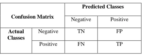
Table 2: Confusion matrix for two class classifier
Confusion Matrix
Predicted Classes Negative Positive
Actual Classes
Negative TN FP
Positive FN TP
The entries in the confusion matrix have the following meaning in the context of our study:
TN is the number of correct predictions that an instance is negative.
FP is the number of incorrect predictions that an instance is positive.
FN is the number of incorrect of predictions that an instance negative, and
TP is the number of correct predictions that an instance is positive [19].
Several standard terms have been defined for the 2 class matrix:
The accuracy (AC) is the proportion of the total number of predictions that were correct. It is determined using the equation 1:
AC= (TN+TP)/(TN+TP+FN+FP) …... (1)
The true positive rate (TP) is the proportion of positive cases that were correctly identified, as calculated using the equation 2:
TP= TP/(FN+TP) …... (2)
The false positive rate (FP) is the proportion of negatives cases that were incorrectly classified as positive, as calculated using the equation 3:
FP= FP/(TN+FP) …... (3)
The true negative rate (TN) is defined as the proportion of negatives cases that were classified correctly, as calculated using the equation 4:
TN= TN/(TN+FP) …... .(4)
The false negative rate (FN) is the proportion of positives cases that were incorrectly classified as negative, as calculated using the equation 5:
FN= FN/(FN+TP) …... (5)
The precision (P) is the proportion of the predicted positive cases that were correct, as calculated using the equation 6:
Fig 2: The predictive accuracy of an algorithms Here we give the comparative analysis of classification accuracy of different data classification algorithm with our proposed approach and we find that the support vector machine gives 96% of classification accuracy, Logistic regression gives the 95% accuracy, perceptron gives the 88% accuracy, Decision tree gives the 93% accuracy of data classification on other hand our proposed approached gives the 97% accuracy of classified data which is shown in fig. 2.
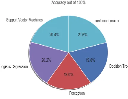
Fig 3: The predictive accuracy rate comparison We also plot the pie chart for predictive accuracy rate for our dataset and we got the accuracy rate out of 100% for Confusion matrix we examine 20.6% which highest accuracy rate, for support vector machine we examine 20.4% which second highest accuracy rate, for logistic regression we examine 20.2% which third highest accuracy rate, for decision tree we examine 19.8% which Fourth highest accuracy rate, and for perceptron we examine 19.0% which lowest accuracy rate of classified data which is shown in fig. 3.
6.
CONCLUSION
This paper has introduced new data classification algorithm which is based PRISM algorithm. We also comparing different algorithm and techniques like SVM, Logistic Regression, Decision tree and perceptron on the basis of that we examine the accuracy rate, our proposed system are simple and easy for implementation likewise first apply classification technique K-fold cross validation on input data secondly rule generation, Exclusion of inefficient rules from rule sets and
predicted rule we added to classify the test data based on induced rules. We performed experiments on animal species data set and we examine efficient accuracy for our predictive proposed algorithm. This approach mainly focused on how would improve efficiency and accuracy, but still there is need to identify the best technique or algorithm for data classification problems.
7.
ACKNOWLEDGMENTS
I would like to thank the College Authorities to provide basic facilities for carrying out the research work. I would like to thank my guide Yogesh Wanjari and my friends for most support, encouragement, timely valuable advices and theme of this paper.
8.
REFERENCES
[1] Cendrowska, J., 1987. “PRISM: An algorithm for inducing modular rules”. International Journal of Man-Machine Studies, 27(4), pp.349-370.
[2] Hadi, W.E., Issa, G. and Ishtaiwi, A., 2017. “ACPRISM: Associative classification based on PRISM algorithm”. Information Sciences, 417, pp.287-300. ELSEVIER.
[3] Hadi, W.E., Aburub, F. and Alhawari, S., 2016. “A new fast associative classification algorithm for detecting phishing websites”. Applied Soft Computing, 48, pp.729-734. ELSEVIER.
[4] Hong, Tzung-Pei, and Shian-Shyong Tseng. "Two-phase PRISM learning algorithms." In Systems, Man, and Cybernetics, 1997. Computational Cybernetics and Simulation., 1997 IEEE International Conference on, vol. 4, pp. 3895-3899.
[5] Bruni, R. and Bianchi, G., 2015. “Effective classification using a small training set based on discretization and statistical analysis”. IEEE Transactions on Knowledge and Data Engineering, 27(9), pp.2349-2361.
[6] Cunhe, L. and Chenggang, W., 2010, May. “A new semi-supervised support vector machine learning algorithm based on active learning”. In Future Computer and Communication (ICFCC), 2010 2nd International Conference on (Vol. 3, pp. V3-638). IEEE.
[7] Martens, D., Baesens, B.B. and Van Gestel, T., 2009. “Decompositional rule extraction from support vector machines by active learning”. IEEE Transactions on Knowledge and Data Engineering, 21(2), pp.178-191.IEEE.
[8] Kesavaraj, G. and Sukumaran, S., 2013, July. A study on classification techniques in data mining. In 2013 Fourth International Conference on Computing, Communications and Networking Technologies (ICCCNT) (pp. 1-7). IEEE.
[9] Jia, Y.S., Jia, C.Y. and Qi, H.W., 2005, August. “A new nu-support vector machine for training sets with duplicate samples”. In Machine Learning and Cybernetics, 2005. Proceedings of 2005 International Conference on (Vol. 7, pp. 4370-4373). IEEE.
[10] Kotsiantis, S.B., Zaharakis, I. and Pintelas, P., 2007. Supervised machine learning: A review of classification techniques. Emerging artificial intelligence applications in computer engineering, 160, pp.3-24.
[image:6.595.58.274.370.536.2]multiple classifier systems (pp. 1-15). Springer, Berlin, Heidelberg.
[12]Abdelhamid, N., 2015. “Multi-label rules for phishing classification”. Applied Computing and Informatics, 11(1), pp.29-46. ELSEVIER.
[13]N. Abdelhamid, A .A . Jabbar, F. Thabtah, “Associative classification common research challenges”. in: 2016 45th Int. Conf. Parallel Process. Work., 2016, pp. 432– 437. IEEE.
[14]D.T. Pham, S. Bigot, S.S. Dimov, “RULES-5: a rule induction algorithm for classification problems involving continuous attributes”. Proc. Inst. Mech. Eng. Part C J. Mech. Eng. Sci. 217 (2003) 1273–1286. ELSEVIER.
[15]Osisanwo, F.Y., Akinsola, J.E.T., Awodele, O., Hinmikaiye, J.O., Olakanmi, O. and Akinjobi, J., 2017. Supervised machine learning algorithms: classification and comparison. International Journal of Computer Trends and Technology (IJCTT), 48(3), pp.128-138.
[16]Liu, H., 2015. Rule Based Systems for Classification in Machine Learning Context, Doctoral dissertation,
University of Portsmouth.
[17] Yogesh Wanjari, Sanjay Nagpure, Gokul Chute, Yogeshwari Kamble, Review on Inclusion of Efficient Rules in PRISM algorithm for Data Classification IJRAR-International Jurnal of Research and Analyatical Reviews, Volume.6, Issue 1, Page No pp.640-642, February-2019.
[18] Wanjari, Y.W., Mohod, V.D., Gaikwad, D.B. and Deshmukh, S.N., 2014, October. Automatic news extraction system for Indian online newspapers. In Proceedings of 3rd International Conference on Reliability, Infocom Technologies and Optimization (pp. 1-6). IEEE.
[19] Santra, A.K. and Christy, C.J., 2012. Genetic algorithm
and confusion matrix for document
clustering. International Journal of Computer Science Issues (IJCSI), 9(1), p.322.
[20] https://en.wikipedia.org/wiki/Machinelearning