ISSN Online: 1947-394X ISSN Print: 1947-3931
DOI: 10.4236/eng.2018.105017 May 16, 2018 253 Engineering
Analysis of Small Oscillations in Complex
Electric Power Systems
Allaev Kaxramon Raximovich, Makhmudov Tokhir Farkhadovich
Department “Electric Stations, Networks and Systems”, Tashkent State Technical University Named after Islam Karimov, Tashkent, Uzbekistan
Abstract
In this article the mathematical model of complex regulated electric system in matrix form is developed. This mathematical model makes it possible to study the steady-state stability of a complex electrical system by determining the ei-genvalues of the dynamics matrix. The model of an electrical system that re-flects transient processes for small deviations is convenient, both algorithmi-cally and computationally, in particular, in cases of their joint solution with steady-state equations—the equations of nodal voltages. The obtained results in the form of the eigenvalues of the matrix spectrum are qualitatively the same as the results of classical studies, which is a consequence of the adequacy of the proposed model and the correct reflection of the dynamic processes occurring in a real electrical system. In addition, the equations obtained are of independent importance for the analysis of various modes, including tran-sient, electrical systems of any complexity.
Keywords
Electric System, Small Oscillations, Automatic Excitation Control, Matrix, Matrix Spectrum
1. Introduction
The present stage in the development of the power industry is characterized by the presence of large concentrated energy systems connected by relatively weak connections, in which the powers of distributed generation are actively included. The change in the composition of generation and the structure of power con-sumption leads to a decrease in the permanent inertia of the elements of the power systems, increasing the sensitivity of the parameters of the regime of the power system as a whole to small perturbations.
How to cite this paper: Raximovich, A.K. and Farkhadovich, M.T. (2018) Analysis of Small Oscillations in Complex Electric Power Systems. Engineering, 10, 253-261.
https://doi.org/10.4236/eng.2018.105017
Received: April 10, 2018 Accepted: May 13, 2018 Published: May 16, 2018
Copyright © 2018 by authors and Scientific Research Publishing Inc. This work is licensed under the Creative Commons Attribution International License (CC BY 4.0).
http://creativecommons.org/licenses/by/4.0/
DOI: 10.4236/eng.2018.105017 254 Engineering
As is known [1][2][3][4], the dynamic properties of complex electrical sys-tems can differ significantly from those of simple electric power syssys-tems (EPS), which is confirmed by numerous field and model experiments and computa-tional and experimental studies. In a multi-machine electrical system, the choice of the parameters of the control devices is much more complicated than in the simplest EPS. Therefore, as a rule, in the case of a multi-machine EPS, one gene-rator or one station is considered to be adjustable and the parameters of their automatic excitation controllers (AECs) are determined based on the task at hand—ensuring equal damping, the required stability factor, etc., and the para-meters of AECs of other stations are assumed to be given, with constant emf. for a certain inductive resistance [2].
In this paper we study the dynamic properties of electrical systems for small deviations (steady-state stability), described by linearized differential equations with constant coefficients.
Verification of the stability of power systems consists in determining the pos-sibility of the existence of a stable regime with small perturbations of the para-meters of the regime with given values of the parapara-meters of the power system, the mode of generating sources, the load of node points, and the tuning of au-tomatic mode control devices [3].
The complication of modern electrical systems, the introduction of digital and logical control devices into their structure requires refined and in-depth studies of the modes of electrical systems. Such a problem can be successfully solved by matrix methods. The article suggests a matrix model of the electric system, solved based on the absolute angles of the generators, which emphasizes the re-levance of the task and the method for solving it [4][5][6].
In the article the mathematical model and equations of multi-machine electric system, resolved concerning absolute angles of load of generators are received. On the basis of the obtained model, the results of steady-state stability analysis will be obtained using the example of a three-generator electric system.
Matrix equations of the elements of the EPS and the whole system were com-piled on the basis of the most widely obtained equations of state variables [4][5] [6], which are small deviations of the mode parameters—the angles of the rotor load of the synchronous generator, busbar voltages, power and other operating parameters of the EPS. The considered matrix equations are used for analysis of transient processes and steady-state stability of EPS and for the synthesis of op-timal parameters of regulators of synchronous machines operating in an elec-trical system.
2. Mathematical Model of Transients in a Complex Electrical
System
DOI: 10.4236/eng.2018.105017 255 Engineering
(
)
[
]
2 2
0
d δi dt = ω Tji PТi−PGi , (1)
where ω0 is the synchronous angular frequency; Tji, , ,δi P PTi Gi-is the inertia
con-stant of the i-th aggregate, the load angle of the i-th generator, the mechanical power of the i-th turbine, the electromagnetic power of the i-th synchronous generator, respectively.
The equation of electromagnetic power of the i-th synchronous generator in the positional idealization has the form [6]:
(
)
2 1
1,
sin n sin ,
Gi ii ii i j ij ij ij
j j i
P E y α E E y δ α
= ≠
= +
∑
− (2)where Ei, Ej—emf. i-th and j-th synchronous generators; yii, yij—intrinsic and
mutual conductivity of the network; αii, αij are complementary angles.
0 0
, , , ,
ij i j i i i j j j ij ij
δ = −δ δ δ δ= + ∆δ δ =δ + ∆δ δ = −δ (3)
and beyond
(
)
(
)
(
)
(
) (
)
0 0 0 0 sin sin sincos cos sin ,
ij ij i i j j ij
i j i j ij
i ij j ij ij
δ
α
δ
δ
δ
δ
α
δ
δ
δ
δ
α
δ
β
δ
β
β
− = + ∆ − + ∆ − = ∆ − ∆ + − − = ∆ − ∆ + (4)
where βij=δi0−δj0−αij.
It should be noted that the derivation of formula (4) uses the obvious rela-tionships:
(
) (
)
(
)
sin ∆ − ∆δi δj ≅ ∆ − ∆δi δj and cos ∆ − ∆δi δj ≅1,
valid for small deviations in the load angles of generators.
After transformations (2), taking into account (3), (4), Equation (1) takes the form:
(
)
2 2 2
0
1,
d i d ji Ti i iisin ii n ij j ii i ij ,
j j i
t T P E y b b c
δ ω α δ δ
= ≠
= − − ∆ + ∆ +
∑
(5)and taking into account the parameters of the initial regime and the relation 0
i i i
δ δ= − ∆δ , finally leads to a differential equation in the deviations:
(
)
2 2
0
1,
d i d ji n ij j ii i ,
j j i
t T b b
δ ω δ δ
= ≠
∆ = ∆ − ∆
∑
(6)where
1, 1,
cos , , , sin ,n n
ij ij ij ij i j ij ii ij ij ij ij
j j i j j i
b a β a E E y b b c a β
= ≠ = ≠
= = =
∑
=∑
(
2 sin)
0.Ti i ii ii ij
P − E y α +c =
In the case of the damper contours of the rotor of the i-th synchronous gene-rator, Equation (6) takes the form:
(
)
(
)
2 2
0
1,
d i d ji n ij j ii i di d i d ,
j j i
t T b b P t
δ ω δ δ δ
= ≠
= ∆ − ∆ − ∆
DOI: 10.4236/eng.2018.105017 256 Engineering
where Pdi is the coefficient of the generalized damper moment of the i-th
gene-rator.
If the deviation of the emf is taken into account. i-th synchronous generator, Equation (7) takes the form [7]:
(
)
(
)
(
)
2 2
0
1,
d i d ji n ij j ii i di d i d d di qi qi .
j j i
t T b b P t P E E
δ ω δ δ δ
= ≠
= ∆ − ∆ − ∆ − ∆
∑
(8)The peculiarity of Equation (8) is that it is allowed with respect to the absolute angles of the system generators and, for example, for the three-generator electric system has the form [6][7][8]:
(
)
(
)
(
)
(
)
(
)
(
)
(
)
(
)
(
)
2 2
1 0 1 11 1 12 2 13 3 1 1 1 1 1
2 2
2 0 2 21 1 22 2 23 3 2 2 2 2 2
2 2
3 0 3 31 1 32 2 33 3 3 3 3 3 3
d d d d d d ,
d d d d d d ,
d d d d d d .
j d q q
j d q q
j d q q
t T b b b P t P E E
t T b b b P t P E E
t T b b b P t P E E
δ ω δ δ δ δ
δ ω δ δ δ δ
δ ω δ δ δ δ
∆ = − ∆ + ∆ + ∆ − ∆ − ∆
∆ = − ∆ + ∆ + ∆ − ∆ − ∆
∆ = − ∆ + ∆ + ∆ − ∆ − ∆
(9) The equations of electromagnetic transient processes in the excitation circuit of the i-th synchronous machine in the deviations have the form [1][2][4]:
(
d d)
,di qi qi qei
T ∆E t = ∆E − ∆E (10)
(
d d)
,ei qei АECi eqi
T ∆E t = ∆U − ∆E (11)
(
d d)
,pi AECi i АECi
T ∆U t = ∆ − ∆e U (12)
where T T Tdi, ,ei pi—the transition time constant of the excitation winding, the
exciter time constant, the automatic excitation controller, respectively;
, ,
qi qei АECi
E E U
∆ ∆ ∆ —deviations of the synchronous, forced emf. and the voltage
at the output of the automatic excitation controller, respectively. The formation of signals via the AEC ∆еi channels in an idealized form (provided that the con-stant times of the differentiating elements of the AEC are considered to be zero) can be represented in the form [9][10]:
(
)
(
2 2)
0 1 2
1 d d d d ,
k
Pk k Pk k Pk k
e k P k P t k P t
∆ =
∑
∆ + ∆ + ∆ (13)where k0Pk, k1Pk, k2Pk are the gain factors of the AEC on the deflection channels,
the first and second derivatives of the regime parameters ΔPk, respectively, k is
the number of adjustable mode parameters.
The advantage of Equations (7) and (8) is their dependence on the deviations of the absolute load angles of the generators (∆δi) rather than the relative angles (∆δij), which provides computational convenience, since these equations can be
joined to the equations of node voltages, whose solutions give absolute angles
[11][12][13][14][15].
DOI: 10.4236/eng.2018.105017 257 Engineering
( ) ( ) ( )
( ) ( )
( ) ( ) ( )
21 22 23
33 34
41 42 42
0 0 0
0 .
0 0
0
n n n n n n n n
n n n n n n n n
n n n n n n n n
n n
n n n n n n
I
A A A
A A A
A A A
× × × × × × × × Σ × × × × × × × × = (14)
The components of the matrix AΣ are defined in [6].
In this case, the vector-column of the state parameters containing the para-meters of the electric system mode has the form:
T
1 n 1 n q1 qn qe1 qen .
x= ∆ δ ∆δ ∆δ∆δ ∆E ∆E ∆E ∆E (15)
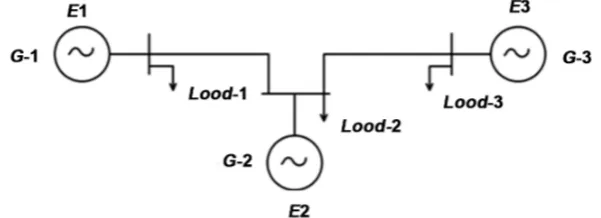
For example, for a three-generator EPS (Figure 1), assuming that the auto-matic excitation regulators react to voltage and load angle deviation of the gene-rators (∆δi, ∆UGi), as well as their first derivatives (∆ ∆δi, UГi).
The equation of the output of the automatic excitation controller for the i-th generator is:
(
)
(
)
0 1 d d 0 1 d d ,
АECi Gi Gi Gi Gi UGi Gi UGi Gi
U kδ δ kδ δ t k U k U t
∆ = ∆ + ∆ + ∆ + ∆ (16)
In this case, the matrix AΣ takes the form [6]:
0 1
11 12 13
1 1
0 2
21 22 23
2 2
3 0
31 32 33
3 3
3 1 1
2 2
3 3
0 1 1
1
0 0 0 1 0 0 0 0 0 0 0 0
0 0 0 0 1 0 0 0 0 0 0 0
0 0 0 0 0 1 0 0 0 0 0 0
d
0 0 0 0 0 0 0 0
d
d
0 0 0 0 0 0 0 0
d
d
0 0 0 0 0 0 0 0
d
1 1
0 0 0 0 0 0 0 0 0 0
1 1
0 0 0 0 0 0 0 0 0 0
1 1
0 0 0 0 0 0 0 0 0 0
0 0 q j q j q j d d d d d d e P E T P E T P E T
A T T
T T
T T
k k
Tδ
ω
ω ω ω
ω
ω ω ω
ω
ω ω ω
− − − − − − − = − − 1 1 1
0 2 1 2
2 2 2
0 3 1 3
3 3 3
,
1
0 0 0 0 0 0 0
1
0 0 0 0 0 0 0 0 0
1
0 0 0 0 0 0 0 0 0
e e
e e e
e e e
T T
k k
T T T
k k
T T T
δ δ δ δ δ − − − (17)
Vector-column of the space of states of parameters of the EPS regime: T 1 2 3 1 2 3 q1 q2 q3 qe1 qe2 qe3 .
x= ∆ ∆ δ δ ∆ ∆ ∆δ δ δ ∆ ∆δ E ∆E ∆E ∆E ∆E ∆E
DOI: 10.4236/eng.2018.105017 258 Engineering Figure 1. Diagram of a three-generator electrical system.
mode and the automatic regulation of the excitation of machines, and therefore fully characterizes the transient processes in this EPS. The matrix A3 is rather sparse, which is typical for a complex system containing n generators, so this fact determines the computational advantages of the proposed mathematical model in the calculation and experimental studies of EPS.
3. Example
As an example, consider the matrix (17) of the intrinsic dynamics of the three-generator electric system A3 (Figure 1). Table 1 shows the technical pa-rameters of the electrical system under consideration.
Where Xd—synchronous inductive resistance of the generator along the
lon-gitudinal axis;
Xc—resistance of branches (inductive resistance of power lines).
The result of the calculation is shown below.
3
0 0 0 1 0 0 0 0 0 0 0 0
0 0 0 0 1 0 0 0 0 0 0 0
0 0 0 0 0 1 0 0 0 0 0 0
235.3565 155.8297 99.8200 0 0 0 0.4167 0 0 0 0 0
104.5232 120.3483 51.6890 0 0 0 0 0.5214 0 0 0 0
50.6447 39.2440 94.1103 0 0 0 0 0 0.5844 0 0 0
0 0 0 0 0 0 1.25 0 0 1.25 0 0
0 0 0 0 0 0 0 1.4286 0 0 1.4286 0
0 0 0 0
A
− −
− −
− −
=
− −
.
0 0 0 0 1.6667 0 0 1.6667
20 0 0 2 0 0 0 0 0 2 0 0
0 0 0 0 0 0 0 0 0 0 2.5 0
0 0 0 0 0 0 0 0 0 0 0 2.2222
−
−
−
−
DOI: 10.4236/eng.2018.105017 259 Engineering Table 1. Parameters of elements of the three-generator power system.
Node number Xd δ0 Tj Xc k0δ k1δ k0u k1u Td Te
1 2 50 5 0.2 10 1 50 3 0.15 1
2 2.2 55 6 0.25 7 2 20 1 0.2 0.5
3 2.195 60 5.5 0.15 8 1 50 2 0.25 0.7
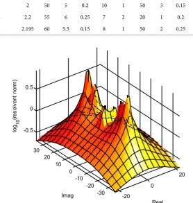
Figure 2. 3D-visualization of the spectrum of a three-generator elec-trical system with a Hurwitz matrix A3.
Similar studies of the stability of complex electrical systems were carried out in [2][5][8], but they used mathematical models derived from the relative an-gles of the load of synchronous generators. In this study, the results were ob-tained with respect to the absolute angles of loads, which allows us to further determine and investigate a particular generator, the first approaching the stabil-ity limit.
Figure 2 shows a 3D visualization of the matrix a pseudo-spectrum obtained with the MATLAB software module EigTool. Note that the EigTool module is a software product developed by Oxford University [15]. Its methodological basis is the method of Arnoldi computation of subspaces of A.N. Krylov [16]. The ho-rizontal axes in Figure 2 correspond to the axes of the complex plane. Logarithm of the norm of the resolvent function was postponed along the vertical axis. Peaks localize the eigenvalues of the matrix.
4. Conclusion
The dynamic properties of complex electrical systems can differ significantly from the properties of simple EPS, which is confirmed by numerous full-scale and model experiments and computational and experimental studies [12] [13]
-20
0
20
-30 -20 -10 0 10 20 30 -0.5
0 0.5
Real Imag
log 10
(res
ol
vent
nor
m
DOI: 10.4236/eng.2018.105017 260 Engineering
[14]. In a multi-machine electrical system, the choice of the parameters of the control devices is much more complicated than in the simplest EPS. Therefore, as a rule, in the case of a multi-machine EPS, one generator or one station is considered to be adjustable and their AEC parameters are determined proceed-ing from the task in hand—providproceed-ing equal dampproceed-ing, the required stability fac-tor, etc., and the parameters of the AEC generators of other stations are selected from the need to provide stability of the entire system and damping of possible oscillations of the regime parameters [17]. Therefore, the introduction of AECs from other generators requires additional studies on the choice of regulatory parameters (synthesis), which is the subject of further research.
References
[1] Abdellatif, B.M. (2018) Stability with Respect to Part of the Variables of Nonlinear Caputo Fractional Differential Equations. Mathematical Communications, 23, 119-126. http://www.mathos.unios.hr/mc/index.php/mc/article/view/2326/526 [2] Klos, A. (2017) Mathematical Models of Electrical Network Systems: Theory and
Applications—An Introduction. Springer International Publishing AG, Berlin. https://doi.org/10.1007/978-3-319-52178-7
[3] Holali, K.D., Efimov, D. and Richard, J.-P. (2016) Interval Observers for Linear Impulsive Systems. 10th IFAC Symposium on Nonlinear Control Systems
(NOLCOS 2016), Monterey, 23-25 August 2016, 867-872.
[4] Kothari, D.P. and Nagrath, I.J. (2003) Modern Power System Analysis. McGraw Hill Education, New York.
[5] Misrihanov, M.Sh. (2004) Klassicheskie i novye metody analiza mnogomernyh di-namicheskih system [Classical and New Methods of Analysis of Multidimensional Dynamic Systems]. Energoatom Publishing, Moskow (In Russian).
[6] Allaev, K.R. and Mirzabaev, A.M. (2016) Matrichnye metody analiza malyh koleba-niy elektricheskih system [Matrix Methods for the Analysis of Small Oscillations of Electrical Systems]. Fan va texnologiya Publishing, Tashkent (In Russian).
[7] Gotman, V.I. (2007) Common Algorithm of Static Stability Estimation and Com-putation of Steady States of Power Systems, Power Engineering, 311, 127-130.
http://www.lib.tpu.ru/fulltext/v/Bulletin_TPU/2007/v311eng/i4/30.pdf
[8] Fazylov, H.F. and Nasyrov, T.H. (1999) Ustanovivshiesya rezhimi elektroenergeti-cheskih sistem i ih optimizaciya [Established Regimes of Electric Power Systems and Their Optimization]. Moliya Publishing, Tashkent (In Russian).
[9] Kovalenko, S., Sauhats, A., Zicmane, I. and Utans, A. (2016) New Methods and Ap-proaches for Monitoring and Control of Complex Electrical Power Systems Stabili-ty. IEEE 16th International Conference on Environment and Electrical Engineering
(EEEIC 2016), Florence, 7-10 June 2016, 270-275.
[10] Allaev, K.R., Mirzabaev, A.M., Makhmudov, T.F. and Makhkamov, T.A. (2015) Matrix Analysis of Steady-State Stability of Electric Power Systems. AASCIT Com-munications, 2, 74-81.
[11] Irwanto, M., et al. (2015) Improvement of Dynamic Electrical Power System Stabil-ity Using Riccati Matrix Method, Applied Mechanics and Materials, 793, 29-33. [12] Anderson, P.M. and Fouad, A.A. (2003) Power System Control and Stability. 2nd
DOI: 10.4236/eng.2018.105017 261 Engineering [13] Kunder, P. (1993) Power System Stability and Control. McGraw-Hill, Inc., New
York.
[14] Pal, M.K. (2007) Power System Stability. Edison, New Jersey.
[15] MATLAB (2001) User’s Guide. Reference Guide. The Math Works, Inc., Natick. [16] Wilkinson, J.H. (1988) The Algebraic Eigenvalue Problem. Clarendon Press,
Ox-ford.